Abstract
Hardness is an essential property in the design of refractory high entropy alloys (RHEAs). This study shows how a neural network (NN) model can be used to predict the hardness of a RHEA, for the first time. We predicted the hardness of several alloys, including the novel C0.1Cr3Mo11.9Nb20Re15Ta30W20 using the NN model. The hardness predicted from the NN model was consistent with the available experimental results. The NN model prediction of C0.1Cr3Mo11.9Nb20Re15Ta30W20 was verified by experimentally synthesizing and investigating its microstructure properties and hardness. This model provides an alternative route to determine the Vickers hardness of RHEAs.
1. Introduction
Refractory high entropy alloys (RHEAs) are designed by adding high melting point elements such as Cr, Mo, Nb, Ta, Ti, V, W, Re, W, Ru, Zr, Rh, Os, Ir, and Hf. RHEAs have excellent properties, such as a high hardness and high-temperature softening resistance [1,2,3,4]. Thus, application of RHEAs can be very promising candidates in the field of aerospace industry. Many studies of RHEAs such as TaNbHfZrTi, TiZrNbMoV, NbMoTaW, VNbMoTaW, Ti2ZrHf0.5MoNbx, and Al0.5CoCrCuFeNi have shown excellent yield strength both at room and high temperatures [5,6,7,8,9,10]. However, the poor ductility at room temperature of RHEAs limits their industrial application. One study has shown that doping elements such as C, B, N, O, Al, Si with RHEAs could improve the mechanical properties of RHEAs and enhance their applications [11,12,13,14,15,16,17,18]. The addition of 0.1 atomic percentage (at.%) of C and 0.3 at.% of C in Mo0.5NbHf0.5ZrTi10 has improved the plasticity and increased the compressive stress [19]. Therefore, doping with low concentrations of non-metallic elements is very important in RHEAs for improving the mechanical properties. However, predicting the mechanical properties of doped RHEAs by the first principles method is very complex. Moreover, experimental techniques are costly and tedious. Therefore, machine learning (ML) could be a promising tool to predict the mechanical properties of new complex RHEAs.
ML approaches have been used to predict the crystal structures and properties of materials [20,21,22] with convincing results. Islam et al. [23] trained neural network (NN) models that can analyze the phase of multi-principal element alloys (MPEAs) with 118 data samples. An NN model is a supervised machine learning prediction model that is inspired by the functionalities of the human brain. Wen et al. [24] developed a material design strategy using ML for predicting the desired properties of high entropy alloys (HEAs). George et al. [25] also utilized a machine learning model which can predict the elasticity of high entropy alloys and included experimental validation. These studies have shown that ML methods are capable and reliable in discovering new RHEAs and predicting their phases. However, many studies focus on phase formation predictions, and a few on predicting the mechanical or functional properties of complex RHEAs.
In this study, the Vickers hardness of several complex RHEAs including C0.1Cr3Mo11.9Nb20Re15Ta30W20 were predicted by utilizing an NN model. We experimentally synthesized C0.1Cr3Mo11.9Nb20Re15Ta30W20, and the phase, microstructure, and Vickers hardness were studied. The measured Vickers hardness was found to be consistent with the NN model prediction.
2. Materials and Methods
2.1. Computational Methods
The features of the alloys and the corresponding target hardness values used in this study were collected from several previous publications [6,19,26,27]. In this study, we only considered the average hardness value of HEAs present in the reference papers and did not consider the hardness value that changed with the applied load. Although a total of 380 experimental records of measured hardness were collected from the literature, the alloys that contained unwanted elements were left out, reducing the number of total available samples to 128.
A supervised machine learning task performs several steps before the actual prediction is made. An NN model requires features to train and thus make informed predictions. In this particular task, 22 relevant features that were initially picked based on the domain knowledge of which features could be helpful to predict Vickers hardness consisted of the percentage of each element in the alloy, i.e., % of Cr, % of Hf, % of Mo, % of Nb, % of Ta, % of Ti, % of Re, % of V, % of W, % of Zr, % of Co, % of Ni, % of Fe, % of Al, % of Mn, % of Cu, % of C, the entropy of the alloy (ΔSmix) [28], the bulk modulus (B), the shear modulus (G), the valence electron concentration (VEC) [29], and the melting temperature (Tm). The HEA features were calculated using the rule of mixtures.
where R is the ideal gas constant, Ci the atomic percentages of the ith element, Bi is the bulk modulus of the ith element, Gi is the shear modulus of the ith element, (Tm)i is the melting point of the ith element, and (VEC)i is the valence electron concentration of the ith element.
In a typical supervised machine learning task, the dataset is split into training and testing sets before any feature engineering, visualization, analysis, or training is performed, so as to prevent any data leakage, i.e., the training should not be influenced by any information from the test data. After random shuffling, 90% of the total samples were allocated for training and validation and 10% for testing. Here, we explain the data preprocessing steps that were conducted on the training data before the NN model was trained. Firstly, the features that had zero or nominal variance were removed from the dataset. The methods adopted for feature selection and engineering in this work stem from a general class of feature engineering techniques [30]. ML models work on the basis of how close the samples are located to each other in the high-dimensional feature space. Features that have nominal variance do not contribute much to differentiating among the samples, therefore it is better to remove such features before passing the data to an ML model to reduce space as well as time complexity. The removed feature was the “% of Re” in each sample, because all the samples in the training data had the same percentage of Re. Next, we removed the correlation among the features by two methods in succession, first, by the method of condition indices, and then by visually plotting the correlation among the features that successfully passed the condition index test.
A subset of the scatterplot of the features before the condition indices step is shown in Figure 1. There is clear association between that bulk modulus, valence electron concentration, entropy, and melting temperature, suggesting that these features are highly correlated. The calculated Pearson’s correlation of coefficient [31] between the RHEA features of 128 samples’ data is shown in Table 1.
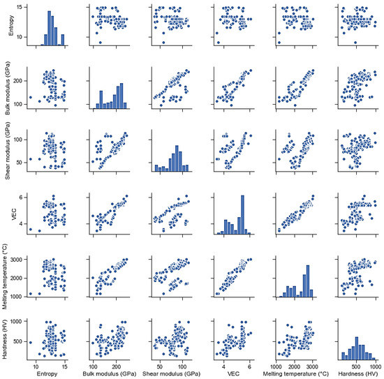
Figure 1.
Scatterplot matrices of six features from the 128 samples data.

Table 1.
The calculated Pearson’s correlation coefficients which are related to different features of high entropy alloys (HEAs) in 128 data samples.
Table 1 shows that a correlation exists among the different features used. During feature removal, only those features that had minimal correlation with the target variable hardness were removed; this set of removed features included VEC, Tm, and B. This is a way to reduce the feature space complexity by losing minimal information from the dataset. Furthermore, visually plotting the scatterplots of the remaining features revealed some correlation among the % of Co, the % of Fe, and the % of Ni. Hence, the % of Co and the % of Fe were eliminated.
Next, Pandas library [32] was used to normalize the value of the features so that each feature came within a range of 0 and 1. Feature normalization allows all the features to scale to a similar scale, and thus makes training faster by balancing the length of the contours of the loss function across all dimensions of the parameters that are to be updated.
After that, the actual training steps began. The number of training samples is very small; therefore, k-fold cross-validation was chosen to obtain a model which performed the best on average among all the validation folds. Furthermore, because a neural network training comes with several hyperparameter choices, the hyperparameters were tuned using a randomized search. The hyperparameter grid used to sample different configurations of randomized hyperparameter search is as below:
learning rate = {0.00005, 0.0001, 0.0003, 0.0005, 0.001, 0.003, 0.005}
weight decay for regularization = {1 × 10⁻⁵, 5 × 10⁻⁵, 1 × 10⁻⁴, 5 × 10⁻⁵, 1 × 10⁻³, 5 × 10⁻³, 1 × 10⁻², 5 × 10⁻², 1 × 10⁻¹}
momentum = {0.5, 0.75, 0.99}
nesterov = {True, False}
number of nodes per layer = {14, 17, 21, 24, 28, 35}
number of maximum epochs to train = {50, 75, 100, 125, 150, 175, 200, 250, 300, 325, 350, 375, 400, 425, 450,475,500}
dropout probability per node = {0, 0.3, 0.5}
minibatch size = {1, 2, 4, 8, 16, 32, 64}
optimizers = {torch.optim.SGD}
The training methodology followed a four-step procedure:
Step 1. Randomly selected 500 different configurations from the hyperparameter space.
Step 2. Trained 500 neural networks using all of these configurations with 20-fold cross validation.
- (a)
- The purpose of this k-fold training was to find the most generalizable set of hyperparameter configurations among the randomly chosen 500 configurations.
Step 3. After obtaining the best set of hyperparameters, we discarded all the previously trained 500 * 20 models and trained a new neural network using:
- (b)
- all the training data;
- (c)
- the best set of hyperparameters obtained from Step 2;
- (d)
- no cross validation. (because we had already found the hyperparameters).
Step 4: In Step 2, all intermediate models were saved at the end of each epoch. This allowed us to monitor the performance of our model on the test set at each epoch. In essence, if the model performance diverged after the nth epoch, we could discard the training epochs after the nth epoch. This gave us the “best model” corresponding to this “best set of hyperparameter configuration”.
The open-source libraries PyTorch, scikit-learn, and scorch were used to train the NN model and predict the hardness of the RHEAs.
The NN model consisted of three abstract regions, namely, the input layer, the hidden layers, and the output layer. The input layer takes in the features and passes them to the hidden layers. The output layer is the last layer of the NN model, which simply produces the output based on the information passed from the last hidden layer nodes. The following relationship can be used to calculate the output of each neuron (aj):
where bj are the bias terms and Wij are the weights provided for each input node. The value of aj proceeds through an activation function. Then, the activation function will define the output of this particular neuron. The type of activation function used in this NN model is leaky ReLU [33]. Figure 2 shows the NN model used in this work, which consisted of five hidden layers. Each layer consisted of different numbers of neurons. A neural network is a universal function approximator, and the larger the network, the more able it is to learn the nuances in the feature space. The weights and biases were randomly initialized before each training. The optimization criterion to optimize was mean square error (MSE) loss.
where n is number of data points, is the observed values, and is the predicted values.
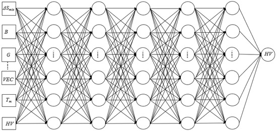
Figure 2.
A schematic model of the neural network (NN) showing 5 hidden layers. The input consists of HEAs features as represented by square boxes on the left.
2.2. Experimental Methods
The C0.1Cr3Mo11.9Nb20Re15Ta30W20 alloy was synthesized by vacuum arc melting method (MAM-1, Edmund Bühler, Bodelshausen, Germany) from the corresponding element mixture under a pure argon atmosphere. The powders of Cr, Mo, Nb, Re, Ta, W, and C were mixed inside a polystyrene mill jar for 15 min and cold pressed in a stainless steel mold using a pressure of 350 MPa and a dwelling time 30 s. The purity of each elements was more than 99.5 wt %. For the purpose of homogeneous distribution of elements, the melted ingots were flipped over and re-melted 4 times. After this, epoxy resin (a mixture of SamplKwick powder and SamplKwick liquid with the volume ratio 2:1) was applied to firmly wrap the solid ingots for easy handling. The cross section of the sample was cut using a BUEHLER low speed saw. Prior to the property tests, the cross section surface was mechanically ground with SiC papers with differing grit sizes, namely, 320, 600, 800, 1000, and 1200 mesh in sequence. After that, the ground cross section surface was polished using the MetaDiTM Supreme polycrystalline diamond suspension (1 μm), and, finally, rinsed with deionized water and dried in air. The crystal structure of the sample was identified using an X-ray diffractometer system (Empyrean, PANalytical) provided with equipped Cu Kα radiation (λ = 0.15406 nm). The 2θ scan range from 20–120 degrees was performed with a step size of 0.026 degrees. The microstructure and chemical compositions of the C0.1Cr3Mo11.9Nb20Re15Ta30W20 were examined using a field emission scanning electron microscope equipped with second electron (SE) and energy dispersive spectroscopy (EDS) detector (Ametek. Model: APOLLO XL, Berwyn, PA, USA). Vickers hardness was measured with a digital micro hardness tester (Clark Instrument Model CM-802AT, Novi, MI, USA). Three testing loads were used, namely, 2000, 500, and 100 gf, and the dwell time was 15 s. The Vickers hardness (HV) of C0.1Cr3Mo11.9Nb20Re15Ta30W20 was tested at five different positions on the sample to ensure the consistency of the results. The intervals between adjacent testing positions were three times larger than that of the indent diagonals, which avoided the effects of work hardening.
3. Results and Discussions
3.1. Machine Learning Results
The best set of hyperparameter configurations obtained were learning rate = 0.001, weight decay for regularization = 0.001, momentum = 0.99, optimizers = stochastic gradient descent, nesterov = True, number of nodes per layer = 35, number of maximum epochs to train = 325, dropout probability per node = 0, and minibatch size = 1. The learning curves of hardness prediction are shown in Figure 3. The y-axis represents the mean squared error and the x-axis represents the number of epochs. It can be seen from the curve that the NN model was able to learn from the training data and predict the hardness of the samples for the validation data with a gradual decrease in loss over several epochs of training, starting from 0.125 and flattening out at around 0.0675. The NN model was trained on a dataset of 128 HEAs. There were also several models that diverged during training. An example case is shown in Figure 4.
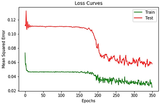
Figure 3.
Learning curves of mean squared error as a function of the number of epochs. The red solid red curve represents the average 20-fold cross-validated loss scores on the validation fold, and the green solid curve corresponds to the 20-fold cross-validated loss score on the training data.
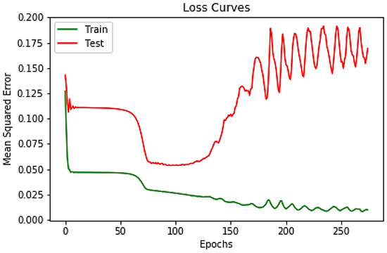
Figure 4.
Mean squared error as a function of the number of epochs: a diverging model.
We also generated, for each test sample, the hardness predictions of all 500 models trained. Then, the uncertainty error bars were plotted using standard deviation as the metric, which are shown in Figure 5. As expected, there existed some variance among the predictions of all 500 models.
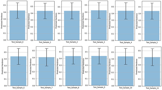
Figure 5.
Error bars for the uncertainty among the trained models on test samples.
The R2 plots of Vickers hardness predicted by the NN on the training and test datasets are presented in Figure 6. As seen, the predictions have a trend along the y = x line. This indicates a good learnability for this task. After testing the model, the predicted hardness of C0.1Cr3Mo11.9Nb20Re15Ta30W20 was found to be 690 HV. In Figure 6b, the training samples also digress from the ideal 45° line. This is because the model used for prediction was chosen to minimize the test loss and not the training loss: we chose the “early-stopped” model as the best model. This can also be observed in Figure 4. Table 2 contains the predicted and experimental Vickers hardness for the HEAs. As seen, the model predictions significantly differ for some samples. This variance is explained by the fact that the number of training samples was limited, and the training set did not contain enough samples from the region in the feature space that some test samples belonged to. This issue could be alleviated by using a large number of training samples from diverse regions in the feature space. We believe that if the NN model is retrained using a higher amount of HEA data, it can predict even better. Therefore, this limitation is not from the model but due to the unavailability of the data.
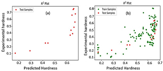
Figure 6.
Hardness prediction by machine learning using the NN model for (a) the testing data and (b) both training and testing data. The red star symbol denotes the predicted hardness of the testing data, and the green star symbol denotes the predicted hardness of the training data.
Table 2.
Experimental and NN model-predicted Vickers hardness of HEAs.
3.2. Experimental Results
The XRD pattern of C0.1Cr3Mo11.9Nb20Re15Ta30W20 with the log intensity y-axis is shown in Figure 7. According to the image, each diffraction peak indicates most likely one single body-centered cubic (BCC) phase. No obviously distinguished peaks can be observed. This indicates the existence of a single-phase BCC phase in C0.1Cr3Mo11.9Nb20Re15Ta30W20. The wavelength of the X-ray is 1.5406 Å. With the help of Bragg’s law [42], described as
where d, θ, n, and λ are interplanar spacing, half of the diffraction angle, positive integer, and X-ray wavelength, respectively. The lattice parameter was determined to be 3.21 ± 0.002 Å.
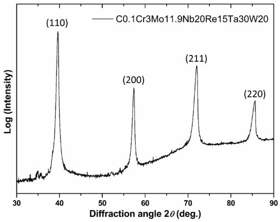
Figure 7.
Image showing the XRD pattern of the alloy, with the x-axis and y-axis indicating the diffraction angle and log function of intensity, respectively.
The microstructure information of the as-cast C0.1Cr3Mo11.9Nb20Re15Ta30W20 alloy is shown in Figure 8a. Two kinds of areas with differing contrast are clearly observed (lighter and darker); the lighter area is larger than the darker area, with the lighter area acting as the matrix and the darker area as the second phase. Interestingly, although two distinguishable areas are seen, the XRD results only show a single BCC phase structure. The two areas are both BCC structures and have almost identical lattice parameters, close enough that they are beyond the detection limit of the XRD device used in this study. The shapes of the darker area are irregular, both particle-shapes (with the size of several micrometers) and strip-shapes (with a width of several micrometers and length up to several tens of micrometers) are observed. A composition test was also performed with EDS. Figure 8b exhibits the nine areas selected for the composition characterization to ensure the reliability of the results, and the composition information is listed in Table 3. Carbon elements were not listed in the table, considering the surface contamination during the polishing and storage processes. Carbon elements would be absorbed on the polished surface from the surroundings, distorting the testing accuracy. Generally, the tested composition of the as-cast alloy was consistent with the nominal composition. However, with a close observation of the table, it is discovered that the tested Cr content is considerably lower than the nominal content. This phenomenon can be explained by the following reason [43,44]: residual oxygen existed in the argon atmosphere; the as-cast alloy surface was inevitably oxidized during the synthesizing process. Cr is beneficial for oxidation resistance by generating dense Cr2O3 layer [45], and the reaction mechanism between Cr and oxygen was reported to be counter-current diffusion of these two elements, which indicates the outward diffusion of Cr during the arc melting process, reducing the Cr content inside the sample on the polished surface.
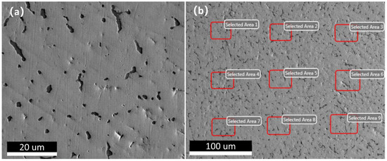
Figure 8.
(a) SEM image of sample surface after polishing; (b) energy dispersive spectroscopy (EDS) testing areas on the sample surface.
Table 3.
EDS testing results of the polished sample surface.
In addition, the difference of vapor pressure among the metal elements is another reason for the variation. As shown in Figure 9, the vapor pressure of the six elements from room temperature to ~2200 °C shows the following relationship [46], Cr > Mo > Nb > Re > Ta > W. Therefore, during the arc melting process, Cr and Mo were more volatile than the other elements, especially Cr.
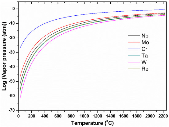
Figure 9.
Image indicating the vapor pressure in log as a function of temperature (from room temperature to around 2200 °C).
An EDS mapping test was also performed to determine the composition distribution in the sample. All the elements except carbon were examined, and the results are displayed in Figure 10. It is clear that the differing contrasts observed in Figure 8a result from element segregation. Elements Nb and Mo are clearly present in the darker areas, while elements Cr and Ta show slightly higher contents in the darker areas. Elements W and Re exhibit opposite behaviors, and mainly exist in the lighter areas. Careful observation of Figure 10 reveals that the lighter areas are likely the dendrites, while the darker areas appear to be inter-dendrite structures. The melting points of W and Re are higher than those of Cr, Nb, Mo, and Ta. During the solidification process of arc melting, elements with higher melting points (W and Re) solidified first, and the elements with lower melting points gradually enriched at the inter-dendrite region. As a result, the segregation of elements was observed.
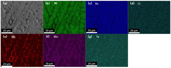
Figure 10.
EDS mapping results of the sample C0.1Cr3Mo11.9Nb20Re15Ta30W20. (a) is the SEM image showing the area for EDS mapping analysis, (b–g) indicate the distribution of W, Re, Cr, Nb, Mo and Ta elements, respectively, on the sample area.
A Vickers hardness test was carried out and the results are listed in Table 4. Based on the results, the average hardness was approximately 600 HV. Meanwhile, it was also determined that with the increase in testing load, the obtained average hardness decreases. This phenomenon is ascribed to indentation size effect [47], and similar observations were also reported by other researchers [48,49].
Table 4.
Vickers hardness test results of C0.1Cr3Mo11.9Nb20Re15Ta30W20.
The ML studies on mechanical and physical properties of HEAs were verified by comparing with the experiments [21,22,23,24,25,26,50,51,52]. The predicted Vickers hardness of C0.1Cr3Mo11.9Nb20Re15Ta30W20 with nominal composition and experimental composition were 695 HV and 686 HV, respectively. The experimentally measured Vickers hardness of C0.1Cr3Mo11.9Nb20Re15Ta30W20 agreed with the machine learning prediction, with an error below 15%. Moreover, the calculated Vickers hardness of C0.1Cr3Mo11.9Nb20Re15Ta30W20 was found to be 900 HV using the rule of mixture and Chen’s model [53]. This predicted value of hardness had an error % of 64, which is not reliable. The hardness predictions from the current model seem very promising because they were studied with small training datasets. The close agreements between predictions and experiments validate the reliability of the current NN model. The prediction accuracy can be further improved with sufficiently larger datasets. A similar neural NN model could be used in predicting properties of future RHEAs, such as yield strength, ductility, and tensile strength, etc.
4. Conclusions
In this study, an NN model consisting of five hidden layers was introduced and the hardness of the novel alloy C0.1Cr3Mo11.9Nb20Re15Ta30W20 was predicted. The microstructure study showed a single BCC phase existing in C0.1Cr3Mo11.9Nb20Re15Ta30W20. The predicted hardness of C0.1Cr3Mo11.9Nb20Re15Ta30W20 by the NN model was 695 HV, which agreed with the experiment. The current NN method will allow researchers to synthesize virtual RHEAs to achieve the expected hardness without any experimental trial and error method. Therefore, provides a promising scope in accelerating RHEAs designs with the desired hardness.
Author Contributions
Conceptualization, U.B., C.Z. (Congyan Zhang) and S.Y.; methodology, U.B. and A.A; software, U.B; C.Z. (Congyuan Zeng), A.A.; validation, C.Z. (Congyan Zhang), S.G. and S.Y.; formal analysis, C.Z. (Congyuan Zeng), and S.G; investigation, U.B., and C.Z. (Congyan Zhang); resources, S.Y.; data curation, A.A., and U.B.; writing—original draft preparation, U.B., C.Z. (Congyuan Zeng) and S.Y; writing—review and editing, S.G. and S.Y; visualization, S.Y.; supervision, S.Y.; project administration, S.Y.; funding acquisition, S.Y. All authors have read and agreed to the published version of the manuscript.
Funding
This research was partially supported by the NSF EPSCoR CIMM project under Award No. 1541079, DOE award No. DE-NA0003979, and DoD support under contract No. W911NF1910005. CZ(Congyuan Zeng) and SG are supported by the US National Science Foundation under grant number OIA-1946231 and the Louisiana Board of Regent for the Louisiana Material Design Alliance (LAMDA). The computational simulations were supported by the Louisiana Optical Network Infrastructure (LONI) with the supercomputer allocation loni_mat_bio15 and 16.
Institutional Review Board Statement
Not applicable.
Informed Consent Statement
Not applicable.
Data Availability Statement
All data and codes used in this study will be made available upon the reasonable request to the corresponding authors.
Conflicts of Interest
The authors declare no conflict of interest.
References
- Soni, V.K.; Sanyal, S.; Sinha, S.K. Phase evolution and mechanical properties of novel FeCoNiCuMox high entropy alloys. Vacuum 2020, 174, 109173. [Google Scholar] [CrossRef]
- Bhandari, U.; Zhang, C.; Yang, S. Mechanical and Thermal Properties of Low-Density Al20+XCr20-XMo20-YTi20V20+Y Alloys. Crystals 2020, 10, 278. [Google Scholar] [CrossRef]
- Tan, X.R.; Zhao, R.F.; Ren, B.; Zhi, Q.; Zhang, G.P.; Liu, Z.X. Effects of Hot Pressing Temperature on Microstructure, Hardness and Corrosion Resistance of Al2NbTi3V2Zr High-Entropy Alloy. Mater. Sci. Technol. 2016, 32, 1582–1591. [Google Scholar] [CrossRef]
- Senkov, O.N.; Scott, J.M.; Senkova, S.V.; Miracle, D.B.; Woodward, C.F. Microstructure and Room Temperature Properties of a High-Entropy TaNbHfZrTi Alloy. J. Alloy. Compd. 2011, 509, 6043–6048. [Google Scholar] [CrossRef]
- Wu, Y.D.; Cai, Y.H.; Chen, X.H.; Wang, T.; Si, J.J.; Wang, L.; Wang, Y.D.; Hui, X.D. Phase Composition and Solid Solution Strengthening Effect in TiZrNbMoV High-Entropy Alloys. Mater. Des. 2015, 83, 651–660. [Google Scholar] [CrossRef]
- Han, Z.D.; Chen, N.; Zhao, S.F.; Fan, L.W.; Yang, G.N.; Shao, Y.; Yao, K.F. Effect of Ti Additions on Mechanical Properties of NbMoTaW and VNbMoTaW Refractory High Entropy Alloys. Intermetallics 2017, 84, 153–157. [Google Scholar] [CrossRef]
- Qiao, D.X.; Jiang, H.; Jiao, W.N.; Lu, Y.P.; Cao, Z.Q.; Li, T.J. A Novel Series of Refractory High-Entropy Alloys Ti2ZrHf0.5VNbx with High Specific Yield Strength and Good Ductility. Acta Metall. Sin. Engl. Lett. 2019, 32, 925–931. [Google Scholar] [CrossRef]
- Brechtl, J.; Chen, S.Y.; Xie, X.; Ren, Y.; Qiao, J.W.; Liaw, P.K.; Zinkle, S.J. Towards a Greater Understanding of Serrated Flows in an Al-Containing High-Entropy-Based Alloy. Int. J. Plast. 2019, 115, 71–92. [Google Scholar] [CrossRef]
- Bhandari, U.; Zhang, C.; Guo, S.; Yang, S. First-Principles Study on the Mechanical and Thermodynamic Properties of MoNbTaTiW. Int. J. Miner. Metall. Mater. 2020, 27, 1398–1404. [Google Scholar] [CrossRef]
- Wang, Z.; Lu, W.; Raabe, D.; Li, Z. On the Mechanism of Extraordinary Strain Hardening in an Interstitial High-Entropy Alloy under Cryogenic Conditions. J. Alloy. Compd. 2019, 781, 734–743. [Google Scholar] [CrossRef]
- Malinovskis, P.; Fritze, S.; Riekehr, L.; von Fieandt, L.; Cedervall, J.; Rehnlund, D.; Nyholm, L.; Lewin, E.; Jansson, U. Synthesis and Characterization of Multicomponent (CrNbTaTiW) C Films for Increased Hardness and Corrosion Resistance. Mater. Des. 2018, 149, 51–62. [Google Scholar] [CrossRef]
- Zhang, H.; Hedman, D.; Feng, P.; Han, G.; Akhtar, F. A High-Entropy B4(HfMo2TaTi)C and SiC Ceramic Composite. Dalt. Trans. 2019, 48, 5161–5167. [Google Scholar] [CrossRef] [PubMed]
- Castle, E.; Csanádi, T.; Grasso, S.; Dusza, J.; Reece, M. Processing and Properties of High-Entropy Ultra-High Temperature Carbides. Sci. Rep. 2018, 8, 1–12. [Google Scholar] [CrossRef] [PubMed]
- Guo, L.; Ou, X.; Ni, S.; Liu, Y.; Song, M. Effects of Carbon on the Microstructures and Mechanical Properties of FeCoCrNiMn High Entropy Alloys. Mater. Sci. Eng. A 2019, 746, 356–362. [Google Scholar] [CrossRef]
- Huang, T.; Jiang, L.; Zhang, C.; Jiang, H.; Lu, Y.; Li, T. Effect of Carbon Addition on the Microstructure and Mechanical Properties of CoCrFeNi High Entropy Alloy. Sci. China Technol. Sci. 2018, 61, 117–123. [Google Scholar] [CrossRef]
- Seol, J.B.; Bae, J.W.; Li, Z.; Han, J.C.; Kim, J.G.; Raabe, D.; Kim, H.S. Boron doped ultrastrong and ductile high-entropy alloys. Acta Mater. 2018, 151, 366–376. [Google Scholar] [CrossRef]
- Lei, Z.; Liu, X.; Wu, Y.; Wang, H.; Jiang, S.; Wang, S.; Hui, X.; Wu, Y.; Gault, B.; Kontis, P.; et al. Enhanced strength and ductility in a high-entropy alloy via ordered oxygen complexes. Nature 2018, 563, 546–550. [Google Scholar] [CrossRef]
- Bagdasaryan, A.A.; Pshyk, A.V.; Coy, L.E.; Konarski, P.; Misnik, M.; Ivashchenko, V.I.; Kempiński, M.; Mediukh, N.R.; Pogrebnjak, A.D.; Beresnev, V.M.; et al. A new type of (TiZrNbTaHf)N/MoN nanocomposite coating: Microstructure and properties depending on energy of incident ions. Compos. Part B Eng. 2018, 146, 132–144. [Google Scholar] [CrossRef]
- Guo, N.N.; Wang, L.; Luo, L.S.; Li, X.Z.; Chen, R.R.; Su, Y.Q.; Guo, J.J.; Fu, H.Z. Microstructure and Mechanical Properties of In-Situ MC-Carbide Particulates-Reinforced Refractory High-Entropy Mo0. 5NbHf0. 5ZrTi Matrix Alloy Composite. Intermetallics 2016, 69, 74–77. [Google Scholar] [CrossRef]
- Agarwal, A.; Rao, A.K.P. Artificial Intelligence Predicts Body-Centered-Cubic and Face-Centered-Cubic Phases in High-Entropy Alloys. JOM 2019, 71, 3424–3432. [Google Scholar] [CrossRef]
- Zhang, Y.; Wen, C.; Wang, C.; Antonov, S.; Xue, D.; Bai, Y.; Su, Y. Phase Prediction in High Entropy Alloys with a Rational Selection of Materials Descriptors and Machine Learning Models. Acta Mater. 2020, 185, 528–539. [Google Scholar] [CrossRef]
- Zhou, Z.; Zhou, Y.; He, Q.; Ding, Z.; Li, F.; Yang, Y. Machine Learning Guided Appraisal and Exploration of Phase Design for High Entropy Alloys. NPJ Comput. Mater. 2019, 5, 1–9. [Google Scholar] [CrossRef]
- Islam, N.; Huang, W.; Zhuang, H.L. Machine Learning for Phase Selection in Multi-Principal Element Alloys. Comput. Mater. Sci. 2018, 150, 230–235. [Google Scholar] [CrossRef]
- Wen, C.; Zhang, Y.; Wang, C.; Xue, D.; Bai, Y.; Antonov, S.; Dai, L.; Lookman, T.; Su, Y. Machine Learning Assisted Design of High Entropy Alloys with Desired Property. Acta Mater. 2019, 170, 109–117. [Google Scholar] [CrossRef]
- Kim, G.; Diao, H.; Lee, C.; Samaei, A.T.; Phan, T.; de Jong, M.; An, K.; Ma, D.; Liaw, P.K.; Chen, W. First-Principles and Machine Learning Predictions of Elasticity in Severely Lattice-Distorted High-Entropy Alloys with Experimental Validation. Acta Mater. 2019, 181, 124–138. [Google Scholar] [CrossRef]
- Gorsse, S.; Nguyen, M.H.; Senkov, O.N.; Miracle, D.B. Database on the Mechanical Properties of High Entropy Alloys and Complex Concentrated Alloys. Data Br. 2018, 21, 2664–2678. [Google Scholar] [CrossRef]
- Zheng, S.; Wang, S. First-Principles Design of Refractory High Entropy Alloy VMoNbTaW. Entropy 2018, 20, 965. [Google Scholar] [CrossRef]
- Zhang, Y.; Zhou, Y.J.; Lin, J.P.; Chen, G.L.; Liaw, P.K. Solid-solution Phase Formation Rules for Multi-component Alloys. Adv. Eng. Mater. 2008, 10, 534–538. [Google Scholar] [CrossRef]
- Guo, S.; Ng, C.; Lu, J.; Liu, C.T. Effect of Valence Electron Concentration on Stability of Fcc or Bcc Phase in High Entropy Alloys. J. Appl. Phys. 2011, 109, 103505. [Google Scholar] [CrossRef]
- A Practical Guide to Dimensionality Reduction Techniques. Available online: https://www.youtube.com/watch?v=ioXKxulmwVQ&ab_channel=PyData (accessed on 12 December 2020).
- Kelleher, J.D.; Mac Namee, B.; D’arcy, A. Fundamentals of Machine Learning for Predictive Data Analytics: Algorithms, Worked Examples, and Case Studies; MIT Press: Cambridge, MA, USA, 2015. [Google Scholar]
- McKinney, W. Python for Data Analysis: Data Wrangling with Pandas, NumPy, and IPython; O’Reilly Media Inc.: Sevastopol, CA, USA, 2012. [Google Scholar]
- Maas, A.L.; Hannun, A.Y.; Ng, A.Y. Rectifier Nonlinearities Improve Neural Network Acoustic Models. Proc. ICML 2013, 30, 3. [Google Scholar]
- Juan, C.C.; Tseng, K.K.; Hsu, W.L.; Tsai, M.H.; Tsai, C.W.; Lin, C.M.; Chen, S.K.; Lin, S.J.; Yeh, J.W. Solution strengthening of ductile refractory HfMoxNbTaTiZr high-entropy alloys. Mater. Lett. 2016, 175, 284–287. [Google Scholar] [CrossRef]
- Zhang, B.; Gao, M.C.; Zhang, Y.; Guo, S.M. Senary refractory high-entropy alloy CrxMoNbTaVW. Calphad 2015, 51, 193–201. [Google Scholar] [CrossRef]
- Senkov, O.N.; Senkova, S.V.; Miracle, D.B.; Woodward, C. Mechanical properties of low-density, refractory multi-principal element alloys of the Cr–Nb–Ti–V–Zr system. Mater. Sci. Eng. A 2013, 565, 51–62. [Google Scholar] [CrossRef]
- Senkov, O.N.; Wilks, G.B.; Scott, J.M.; Miracle, D.B. Mechanical properties of Nb25Mo25Ta25W25 and V20Nb20Mo20Ta20W20 refractory high entropy alloys. Intermetallics 2011, 19, 698–706. [Google Scholar] [CrossRef]
- Stepanov, N.D.; Shaysultanov, D.G.; Salishchev, G.A.; Tikhonovsky, M.A.; Oleynik, E.E.; Tortika, A.S.; Senkov, O.N. Effect of V content on microstructure and mechanical properties of the CoCrFeMnNiVx high entropy alloys. J. Alloy. Compd. 2015, 628, 170–185. [Google Scholar] [CrossRef]
- Chen, S.Y.; Yang, X.; Dahmen, K.A.; Liaw, P.K.; Zhang, Y. Microstructures and crackling noise of AlxNbTiMoV high entropy alloys. Entropy 2014, 16, 870–884. [Google Scholar] [CrossRef]
- Zhuang, Y.X.; Liu, W.J.; Chen, Z.Y.; Xue, H.D.; He, J.C. Effect of elemental interaction on microstructure and mechanical properties of FeCoNiCuAl alloys. Mater. Sci. Eng. A 2012, 556, 395–399. [Google Scholar] [CrossRef]
- He, J.Y.; Liu, W.H.; Wang, H.; Wu, Y.; Liu, X.J.; Nieh, T.G.; Lu, Z.P. Effects of Al addition on structural evolution and tensile properties of the FeCoNiCrMn high-entropy alloy system. Acta Mater. 2014, 62, 105–113. [Google Scholar] [CrossRef]
- Cullity, B.D. Elements of X-ray Diffraction; Addison-Wesley Publishing: Boston, MA, USA, 1956. [Google Scholar]
- Trindade, V.B.; Krupp, U.; Wagenhuber, P.E.G.; Christ, H.J. Oxidation Mechanisms of Cr-Containing Steels and Ni-Base Alloys at High-Temperatures--. Part I: The Different Role of Alloy Grain Boundaries. Mater. Corros. 2005, 56, 785–790. [Google Scholar] [CrossRef]
- Tsai, S.C.; Huntz, A.M.; Dolin, C. Growth Mechanism of Cr2O3 Scales: Oxygen and Chromium Diffusion, Oxidation Kinetics and Effect of Yttrium. Mater. Sci. Eng. A 1996, 212, 6–13. [Google Scholar] [CrossRef]
- Kuhn, B.; Talik, M.; Niewolak, L.; Zurek, J.; Hattendorf, H.; Ennis, P.J.; Quadakkers, W.J.; Beck, T.; Singheiser, L. Development of High Chromium Ferritic Steels Strengthened by Intermetallic Phases. Mater. Sci. Eng. A 2014, 594, 372–380. [Google Scholar] [CrossRef]
- Alcock, C.B.; Itkin, V.P.; Horrigan, M.K. Vapour pressure equations for the metallic elements: 298–2500K. Can. Metall. Q. 1984, 23, 309–313. [Google Scholar] [CrossRef]
- Uzun, O.; Karaaslan, T.; Keskin, M. Hardness Evaluation of Al-12Si-0.5 Sb Melt-Spun Ribbons. J. Alloy. Compd. 2003, 358, 104–111. [Google Scholar] [CrossRef]
- Uzun, O.; Karaaslan, T.; Gogebakan, M.; Keskin, M. Hardness and Microstructural Characteristics of Rapidly Solidified Al-8-16 Wt.% Si Alloys. J. Alloy. Compd. 2004, 376, 149–157. [Google Scholar] [CrossRef]
- Xu, B.; Tian, Y. Ultrahardness: Measurement and Enhancement. J. Phys. Chem. C 2015, 119, 5633–5638. [Google Scholar] [CrossRef]
- Chang, Y.J.; Jui, C.Y.; Lee, W.J.; and Yeh, A.C. Prediction of the composition and hardness of high-entropy alloys by machine learning. JOM 2019, 71, 3433–3442. [Google Scholar] [CrossRef]
- Bhandari, U.; Rafi, M.R.; Zhang, C.; Yang, S. Yield strength prediction of high-entropy alloys using machine learning. Mater. Today Commun. 2020, 101871. [Google Scholar] [CrossRef]
- Zhao, Q.; Yang, H.; Liu, J.; Zhou, H.; Wang, H.; Yang, W. Machine learning-assisted discovery of strong and conductive Cu alloys: Data mining from discarded experiments and physical features. Mater. Des. 2020, 197, 109248. [Google Scholar] [CrossRef]
- Tian, Y.; Xu, B.; Zhao, Z. Microscopic theory of hardness and design of novel superhard crystals. Int. J. Refract. Met. Hard Mater. 2012, 33, 93–106. [Google Scholar] [CrossRef]
Publisher’s Note: MDPI stays neutral with regard to jurisdictional claims in published maps and institutional affiliations. |
© 2021 by the authors. Licensee MDPI, Basel, Switzerland. This article is an open access article distributed under the terms and conditions of the Creative Commons Attribution (CC BY) license (http://creativecommons.org/licenses/by/4.0/).