1. Introduction
The heteroepitaxial growth of semiconductors on lattice-mismatched substrates is becoming a viable path to improve the performances and add functionalities of electronic and optoelectronic devices [
1]. However, due to the lattice mismatch, a plastic relaxation via injection of dislocations is unavoidable above a certain critical thickness [
2].
For the common case of a uniform composition film grown on a (001)-oriented substrate, the relaxation process has been widely investigated and described in detail. Provided that the lattice mismatch is around
or below [
3,
4], dislocations nucleate as (semi-)loops near the free surface and expand under the effect of the heteroepitaxial stress field, depositing a segment of misfit dislocation (MD) at the heterointerface bounded by its associated threading arms (TDs). These TDs then run through the layer progressively relieving the misfit strain. The residual gliding force on them decreases and they eventually stop encountering other defects or local stress field fluctuations [
5,
6,
7]. By appropriate annealing procedures this relaxation process can be pushed toward nearly the full relaxation of the layer, with the final dislocation microstructure resulting in a nearly perfectly-ordered network of MDs placed at the heterointerface [
8], approaching the thermodynamic minimum-energy configuration [
9].
However, by direct growth of uniform composition films, two major problems arise: (a) the threading dislocation density (TDD) can be reduced only down to a certain saturation value [
10,
11,
12], degrading the expected advantages from the superior material qualities [
13] and (b) the deposition of a largely mismatched film can trigger phenomena such as formation of three-dimensional islands (see, e.g., [
14,
15,
16]), possibly leading to substrate digging and intermixing [
17,
18,
19,
20]. While such islands display extremely interesting shapes and growth modalities [
21,
22,
23,
24] and can lead to quantum confinement [
25], there also exist several applications where a flat layer is preferred. Between all the alternatives proposed to overcome these limitations, the most straightforward is compositional grading [
26,
27]. This consists in gradually increasing the mismatch during the growth by slowly varying the concentration of the main stressor. Grading allows for the possibility to lower the typical TDD by at least one order of magnitude with respect to its constant-composition layer counterpart [
4], but in spite of its well-established success, the optimization of the growth parameters requires a still-lacking understanding of the resulting MDs distribution.
This is complicated by the physics of dislocations: they are atomistic defects but can exhibit collective behavior up to the mesoscale [
28,
29] due to the long-range nature of their interactions. At this scale the effectiveness of typical atomic-scale experimental technique like Transmission Electron Microscopy (TEM) are hindered by statistics and thus theoretical investigations plays a major role in coadiuvate experimental findings [
30,
31,
32,
33]. Several studies have been proposed to address the problem of finding minimum-energy dislocation configurations. In particular, the model proposed by Tersoff [
34] (see also the corresponding Erratum, Ref. [
35]) is often accepted as reference for understanding the effect of a linearly-graded concentration profile on the equilibrium distribution of misfit dislocations. Particularly, Tersoff model provides the solution in terms of a mean-field dislocation density, finding that dislocations tend to occupy nearly the whole layer thickness, and are not confined anymore at the heterointerface. Further developments have been also proposed in order to extend his approach to arbitrary compositional profiles [
36].
Here, we present a computational investigation that goes beyond the Tersoff mean-field model by addressing the N-body problem of interacting dislocations, thus retaining information at the level of single dislocation positioning. In doing so, we exploited convenient analytical expressions for the non-singular, periodic stress field of dislocations near a free surface. Those formulae were exploited in the Peach–Kohler equation for searching low energy dislocation configurations by a steepest-descent procedure. In order to define physical meaningful quantities we used typical parameters describing SiGe/Si(001), a prototypical system.
We carried out applications to the uniform composition layers in order to validate the approach against well-known results. Then, attention was dedicated to investigating graded layers focusing our attention on the linear grading, by far the most common system in experimental investigations [
26,
27,
37]. A careful comparison with the model proposed by Tersoff is provided, but the possibility to retain the information about the positioning of single defects allows our model to explore in more details the dislocation microstructures with respect to mean-field approaches. In particular, the transition between the 2D network of dislocations placed at the heterointerface observed in uniform composition layers to the 3D dislocation microstructures observed in graded layers was directly observed reproduced and discussed. Furthermore, we carried out a critical analysis of the lowest-energy configuration obtained in the case of linear grading. Indeed, several experimental investigations [
37,
38,
39] showed the importance of Frank–Read (FR) or modified FR sources on the formation of the dislocation microstructures typically observed in graded layers. These are commonly described as purely kinetic processes but, as we demonstrated, there exists also a thermodynamic driving force leading to the formation of very similar dislocation distributions in graded layers.
2. Theoretical Methods
The aim of this work is to understand low-energy dislocation distributions in compositionally- graded layers. We used the SiGe/Si(001) system as reference and in all calculations we exploited linear elasticity theory and considered isotropic approximation. The Young modulus and the Poisson ratio used were
GPa and
, respectively. Furthermore, we considered a two-dimensional (2D) system with MDs modeled as infinite straight defects with dislocation line lying along a direction orthogonal to the simulation cell. This greatly simplifies the analysis and allow us a direct comparison with previously reported models [
34,
36,
40]. However, this assumption neglects the presence of the orthogonal dislocation array relaxing strain in the other direction and thus attention should be taken before comparing our results with experimental works, as will be discussed later in the paper.
Energy calculations were performed by numerical integration of the elastic energy density
, with
and
the stress and strain tensors. During this procedure, particular care has been taken in order to correctly follow the rapid variations of stress/strain fields near dislocation cores. For every configuration, an ad-hoc and locally-refined 2D mesh has been generated so that higher spatial resolution was used for the regions near dislocation cores (see also Ref [
24] for an example of the mesh generator used).
A standard steepest-descent procedure was exploited to explore the configurational space, locating local energy-minima for distributions of dislocations initialized with an assigned number of defects randomly introduced in the layer. The force governing dislocation motion as response to an applied stress field is given by the Peach–Koehler expression [
41]:
with
direction of the dislocation line,
the Burgers vector of the considered dislocation and
the local stress field. This expression can be obtained considering a change of the dislocation line configuration
at each point on the dislocation line itself. The quantity
defines the variation in energy of the system per unit length. In this sense, Equation (
1) represents the negative derivative of the dislocation energy with respect to dislocation line motion [
42], considering effects from both glide and climb. The stress field consists, in our case, of two main contributions: the heteroepitaxial stress field due to the lattice mismatch and the stress produced by the other defects. The former can be evaluated in linear elasticity by solving the plane stress problem for a layer subject to an applied biaxial strain
due to lattice mismatch with respect to the Si substrate
with
Å and
Å. Vegard’s law was assumed for evaluating
at whatever Ge concentration considered. The stress field produced by dislocations requires two main difficulties to be taken care of: the traction-free surface condition and the divergence at dislocation cores. In the special case under consideration of 2D thin heterolayers with flat free surfaces, both of them can be addressed analytically. In particular, we exploited the stress field functions reported in
Appendix A, firstly derived in Ref. [
43]. Those are periodic expression obtained by summing individual dislocation contributions taken from the solution proposed by Head [
44] for the free surface problem and the non-singular expressions by Cai and coworkers [
45]. These latter are obtained by smoothing isotropically the Burgers vector density around the dislocation line. By exploiting the above described formula it is not needed to rely neither on explicitly truncated sums for the periodicity neither on numerical solutions for the free-surface problem [
24,
46]. This particular approach also present the advantage of being self-consistent with the Peach–Koehler expression [
45], which represents the negative derivative of the elastic energy and contains both climb and glide components. The simple form of Equation (
1) may therefore be retained, unlike what happens in other approaches, for example the one from Gavazza and Barnett [
47]. Notice that the use of periodic stress functions automatically imposes periodic boundary conditions (PBCs) to the simulation cell.
In Face Centered Cubic (FCC) crystals (like SiGe), dislocations with Burgers vector belonging to the
family are known to be the main kind of perfect dislocations. These are the defects with the lowest magnitude of the Burgers vector which belong to glide planes corresponding to the close-packed ones for FCC crystals [
48]. Thus, in our work we considered two possible Burgers vectors,
, and
, whose components are expressed in the normalized conventional cell coordinate system. Dislocation line has been taken along the
direction and for Si
nm [
3].
and
dislocations can react and give a third kind of defect with Burgers vector
, which has pure edge character. While providing the same amount of biaxial strain relaxation,
defects reduce the total dislocation energy by Frank criterion [
41]. We allowed this process to happen in our simulation by replacing
and
dislocations with a
edge one whenever their distance was closer than a critical radius of about
nm.
Even though dislocations are introduced in a fairly complicated manner during a real growth process, a search for a local energy minimum could start in principle from any arbitrary (albeit reasonable) distribution. Therefore we used, for every composition profile and for every assigned number of dislocations, several initial random configurations, in order to avoid biases when sampling the energy landscape. For each initial condition we performed an unconstrained steepest descent algorithm, collecting statistics for understanding the common features of the energy minima.
Finally, when constant composition layers or stepped profiles are used, the discontinuous Ge concentration at each interface has been smoothed using a Fermi Dirac-like expression:
where
is the fractional increase in Ge content among the considered interface,
is the interface
y coordinate. This was done in order to avoid numerical inconsistencies in energy calculations and instabilities in the steepest descent algorithm.
represents an offset parameter of the order of few nanometers that allow for the
c variation at
to be
. Since we simulated cells much bigger than the length scale of the composition smoothing, the actual value of the offset parameter has no impact on the results.
3. Results and Discussion
In this section we present the results obtained by applying the above described procedure to the study of the minimum-energy dislocation configurations in strained SiGe/Si layers. Two notable cases are considered: the constant-composition layer, discussed in
Section 3.1, and the linearly-graded layer, analyzed in
Section 3.3. As discussed before, the force governing dislocation motion is expressed by the Peach–Kohler force of Equation (
1). In the systems under consideration the local stress tensor
consists of two contributions, the heteroepitaxial stress field and the stress produced by other defects (including in a general sense also the free surface effect as an interaction with “image” dislocations, fully considered by our stress expressions of
Appendix A.1). The combined effect of these two driving forces, as we shall directly show, determines the behavior of the dislocation distribution. In order to better elucidate this concept we will also include the analysis of the minimum energy configurations in step-graded concentration profiles in
Section 3.2. This was specifically designed to represent a bridge between the constant composition layer for a single concentration step and the linear grading in the limit of infinite number of steps.
3.1. Constant Composition Layer
In
Figure 1 we show examples of the application of our unconstrained steepest descent minimization procedure to the case of a constant composition SiGe layer. In order to compare results with parameters typically encountered in experimental conditions, we set the thickness of the layer at
nm and the composition
, as in Refs. [
32,
33] (in such references the nominal concentration is
, we used
only to get a rounded number when exploring multiples of
in
Section 3.2). This choice of parameters corresponds to a high overcritical film, the thickness of the layer being almost 10 times higher than the critical thickness predicted by the Matthews and Blakeslee model (
, see e.g., Ref [
3], p. 14).
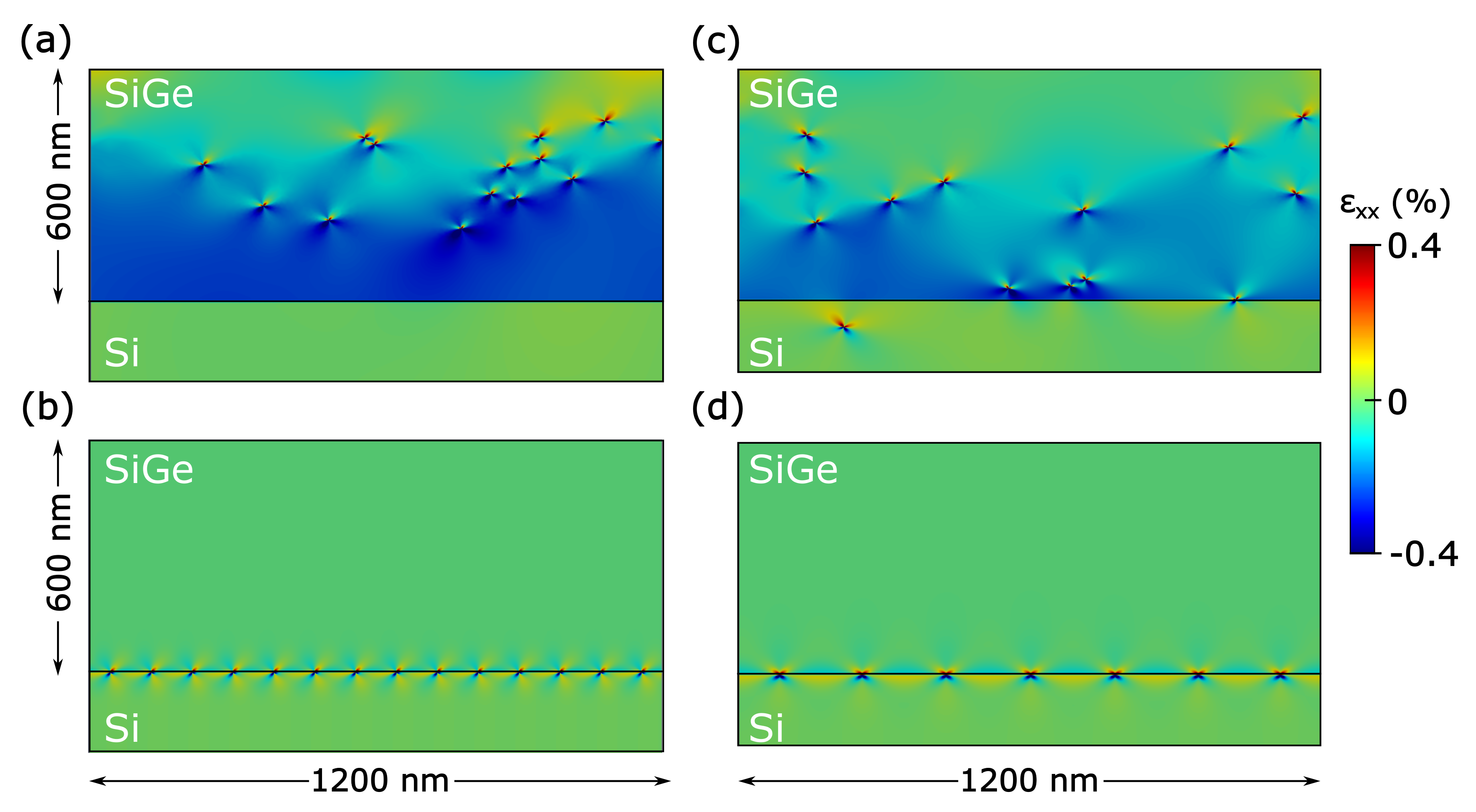
Figure 1a,b show, respectively, examples of the starting condition and the final result of a simulation with a random distribution of 14 dislocations, all taken with the same Burgers vector
. This number has been chosen in order to ensure full relaxation of the SiGe layer. As we explicitly verified by energetic evaluations this condition corresponds to the minimum-energy configuration for such a high overcritical film. The number of defects required to achieve zero net strain in the layer can therefore be estimated as
, where
is the mismatch between pure Si and pure Ge,
is the concentration of Ge and
is the projection of the Burgers vector on the direction providing strain relief. This can be confirmed by inspection of the strain maps in
Figure 1b,d.
Despite sampling several initial conditions, the procedure leads to a unique minimum energy configuration for all the random starting conditions simulated (100) and shows, as expected, a perfectly ordered array of dislocations lying at the SiGe/Si interface. The distance between the defects in the array is close (by construction) to the optimal value
, ensuring on average full relaxation of the strain in the layer, as confirmed by the strain map of
Figure 1b. This results is well known in heteroepitaxy, and, while experimentally deviations from this simple picture are often encountered [
32,
33,
49], it is often reported as a useful first approximation of the expected distribution of dislocations [
4].
This result does not change drastically when considering distribution of dislocations with the two possible Burgers vector considered,
and
. In
Figure 1c,d we report initial and final condition of a simulation on the same SiGe/Si system discussed above but by taking in this case 14 dislocations with an equal distribution between the
and
Burgers vectors. In this situation, as discussed in
Section 2, we also modeled the reaction between two defects with different
into a single edge dislocation [
50,
51]. In this case, different local energy minima can be found depending on the starting condition, and the result of
Figure 1d represents the lowest-energy configuration found. A single array of edge dislocations placed at the SiGe/Si interface is produced, with all the 14 initial defects coalescing into 7 edge dislocations. The spacing of defects in this case is obviously doubled with respect to the value
found before. Experimental evidences showing this minimum energy configuration are usually hindered by the kinetics of dislocation reactions, requiring the activation of high-energy processes like the climb motion of dislocations. Notably, however, thanks to a dedicated two-temperature growth of a high-strained Ge/Si layers, Sakai and coworkers demonstrated the formation of a nearly perfectly-ordered array of pure-edge dislocations [
8], reaching in experiments a result analogous to the configuration found here. Notice that this justifies a fortiori our two-dimensional model: the dislocation array relaxing strain in one direction does not seem to significantly influence the orthogonal dislocation array relaxing strain in the other direction.
3.2. Step Graded Profiles
In order to understand the competition between the driving forces leading to the shape of the dislocation distribution inside a graded layer, we exploited a procedure yielding the linear graded profile as the limit of an increasing number of concentration steps. Given a final concentration
, we subdivided a layer of total thickness
nm into
N steps, each one with a thickness of
and a Ge concentration of
, with
. Notice that the actual concentration value
is reached only in the limit of infinite number of layers
, while if
we recover the case of a single composition layer with a Ge concentration of
. Thus, we can directly compare the results obtained by this approach with the ones obtained for the constant composition layer discussed in
Section 3.1 by taking
, double the value of the Ge concentration used before,
. Among the possible ways of decomposing a linear grading profile into a step graded one, the procedure here proposed has the advantage of maintaining on average the same Ge content in the layer.
In
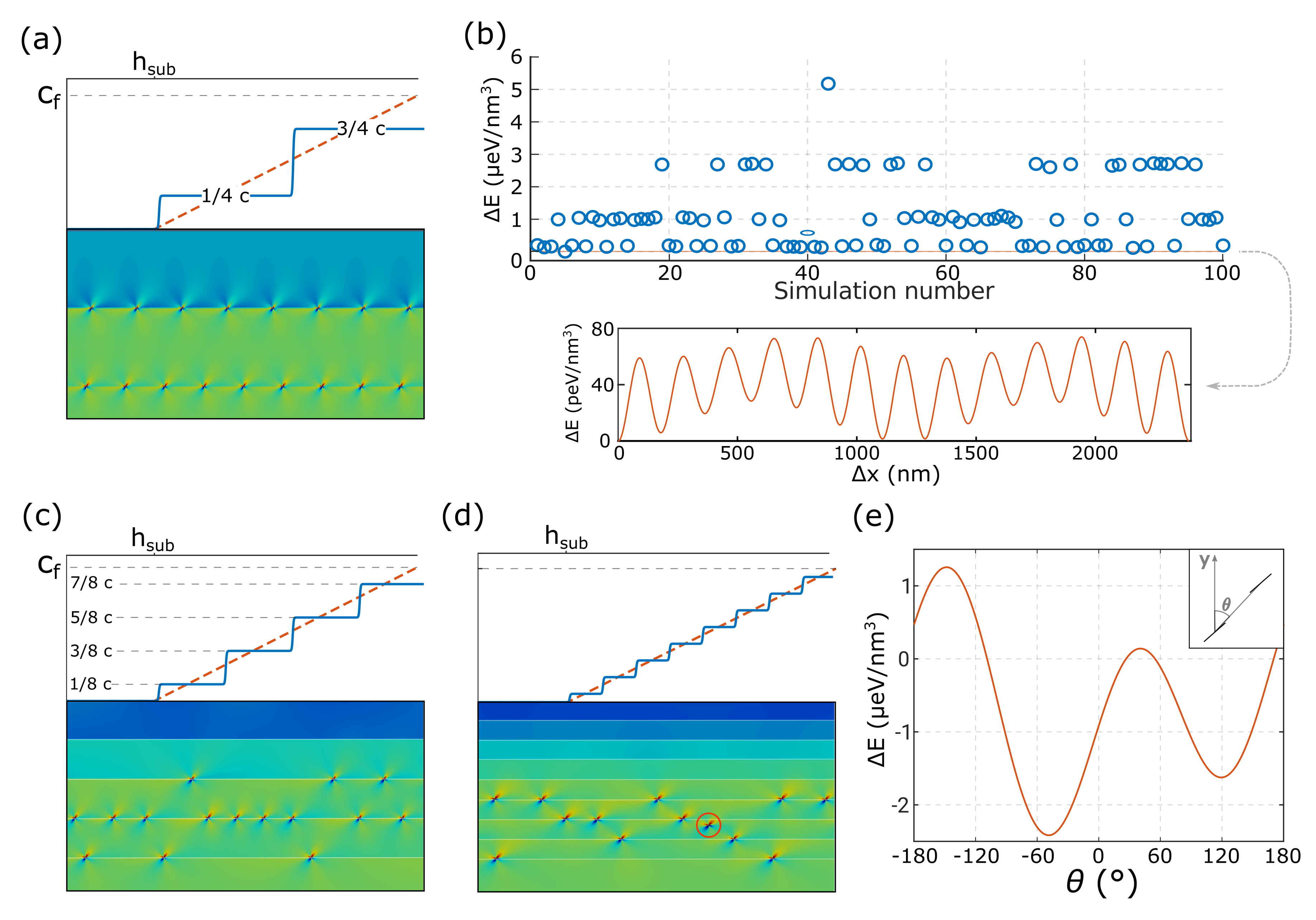
Figure 2 we report the results obtained by applying the same minimization procedure introduced in
Section 2 to the case of step-graded concentration profiles with
, and 8. In this case, to ensure a reliable statistic we doubled the total dimension of the simulation cell (2400 nm) and the total number of dislocations (28). The density of dislocations remains the same as discussed above for the constant composition layer. In all the simulations here reported we started again from random dislocation distributions inside the simulation cell and we obtained the local minima by means of the steepest descent procedure.
In the 2-layer case reported in
Figure 2a, we can see that dislocations tend to place themselves at the interfaces between the concentration steps forming equally-spaced arrays with their relative positions nearly “decoupled”. This concept can be better appreciated by looking at
Figure 2b. There, we plot all the energy minima obtained by considering 100 different random initial conditions. A large number of different local minima were obtained as the result of the steepest descent, contrary to the uniform composition case of
Figure 1a,b. Furthermore, we can observe that the local minima are mainly positioned within discrete energy levels, corresponding to dislocation configurations with different number of defects distributed among the two interfaces of the two-step profile of
Figure 2a. However, once identified a local minimum, a rigid shift of the upper array with respect to the lower one produces negligible fluctuations in energy, about 5 orders of magnitude smaller than the range of the plot. These cannot be distinguished in the top plot of
Figure 2b (here visible as a red line) and thus in the inset of the image we show the energy dependence on a suitable scale. In this terms we can say that the positions of the two arrays of dislocations of
Figure 2a are “decoupled” and the interaction between them is negligible.
In
Figure 2c we show one typical result obtained by the minimization procedure in a 4-step concentration profiles. As can be seen from the picture, dislocations still tend to place themselves at the interfaces between concentration steps. However, due to the reduced thickness of the layers, the interaction between them is now more pronounced, breaking the perfect ordering of the defects within the single arrays.
Finally, in
Figure 2d the 8-concentration step case is reported. In this case the effect of mutual dislocation interaction is even more pronounced, leading the defects to eventually place outside of the interfaces between concentration steps, as exemplified by the red-circled dislocation. The dislocations are now free to place themselves at the minimum energy configuration resulting from the interaction with the neighboring defects. In this way, they align in structures known as pileups of MDs [
37]. This is proved in
Figure 2e, where we show additional calculations showing the energy dependence with respect to the angle between two dislocations in absence of the heteroepitaxial field. These were obtained by keeping the distance between the dislocations at
nm and moving one defects with respect to the other (fixed at 600 nm from the free surface). The optimal angle found for the interaction between these two defects turns out to be about
with respect to the
y-axis, very close to the angle of the pileup in
Figure 2d.
Based on the so far obtained results the following scenario can be drawn: when dislocations are forced to place into positions where different arrays are slightly interacting between them, they tend to “fill up” horizontally-ordered arrays placed at the interfaces between the concentration steps. These arrays, on average, relax the concentration steps of the layers one at a time starting from the bottom. Then, as our step-graded procedure tends towards the linear grading profile, the strong confinement of defects at the interfaces vanishes and the effect of dislocation–dislocation interaction became more visible, with the formation of dislocation pileups as a result. Thus, even if the here-described concentration profiles are seldom used in the growth of heteroepitaxial layers, we introduced them in order to directly show the competition between the different driving forces acting on the dislocations, facilitating the understanding of their behavior in linear graded layers.
3.3. Linear Grading
After having discussed in detail the behavior of dislocation complexes in step-graded profiles in the previous section, we can move now our discussion towards the linear graded profile. We will start by extending the concept of filling up of the dislocation arrays discussed above in the case of linear grading by describing the optimal position of a single dislocations inserted in a overcritical layer with a linearly-graded composition profile and then move towards more complex scenarios by increasing the number of defects in the simulation cell and by discussing the role of the Grading Rate (GR). We will also discuss how our results can be compared with the Tersoff model [
34] by introducing some properly-designed descriptors for the distribution of dislocations.
3.3.1. Single Dislocation
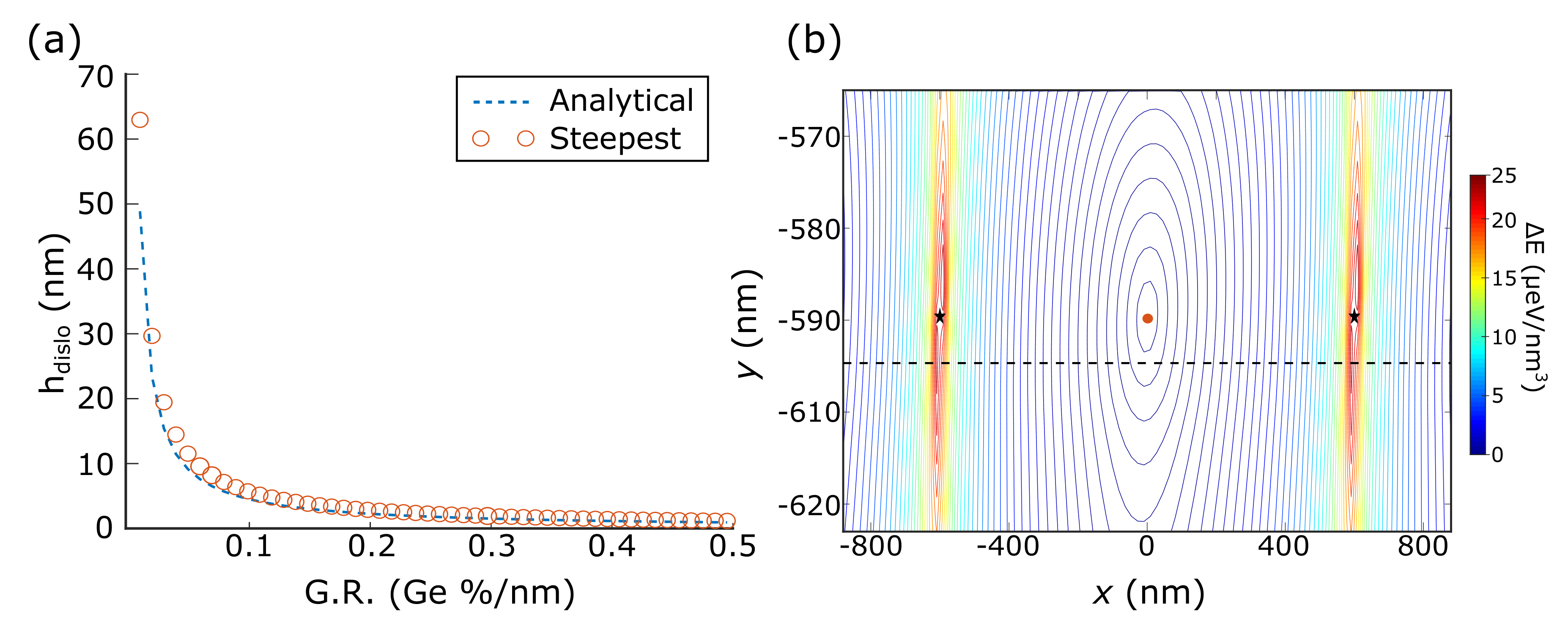
The equilibrium position of a single dislocation in an overcritical layer with linearly-graded concentration profile is not trivially located at the SiGe/Si interface as in the uniform composition case. It results from the equilibrium between the image force acting due to the traction-free free surface condition and the linearly increasing heteroepitaxial field, yielding an equilibrium position at a certain value above the interface. In our approach, this value can be estimated by placing the dislocation inside the simulation cell and finding its equilibrium position by means of the steepest descent procedure. In
Figure 3a, we report the results obtained for a 600 nm-thick cell as function of the GR, plotted as red circles. Here, non-periodic (but still non-singular) stress functions have been used.
Furthermore, the same result can be obtained analytically by balancing, as explained, the image force and the force due to the heteroepitaxial strain. Given the distance
l forms the free surface, we can express the first contribution as [
48]:
where
is the angle between the dislocation line and the Burgers vector and
the second Lamé constant. The approximation used here consists in considering the distance from the free surface much bigger than the dislocation core radius
, then
reducing the dependence to a simple inverse proportionality. The second contribution can be expressed through the Peach–Koehler expression (
1) as:
with
the first Lamé constant. The minus sign arises from the fact that this force pulls the dislocation towards the bulk,
is the final Ge concentration,
is the
y coordinate of the Si/SiGe interface, and
is the misfit between pure Si and pure Ge. Setting the total force equal to zero yields a quadratic equation, whose solution reads:
This expression yields the same result of the one based on energy minimization in Ref. [
52], if, instead of the critical thickness, the full thickness of the film
is used. An approach closer to our line of reasoning can be found in Ref. [
53], where an analogous expression stemming from force balance is reported, together with a discussion on the second root of the quadratic equation. In
Figure 3a the values obtained from Equation (
5) are plotted as a blue dashed line, compared with the steepest descent calculations. The two results are in close agreement.
The situation does not vary significantly when periodic functions are used. In
Figure 3b we show a contour plot of the energy surface for a system hosting one (periodic) dislocation. The positions of the dislocation and its first periodic image are marked in the figure with a star symbol. As can be seen in the figure, the equilibrium position of this dislocation lies about 10 nm above the interface (marked by a black dashed line). Furthermore, from the contour plot it is possible to observe the presence of a single minimum energy position inside the simulation cell (marked by a red circle in the image). This would be the equilibrium position for the introduction of a further dislocation, aligned at the same
y level of the first one. These results extend the idea of filling up of the dislocation arrays described for the step-graded profiles to the linear grading. Thus, in a largely-overcritical film whose misfit is only slightly plastically relaxed, dislocations tend to horizontally fill ordered arrays of defects positioned slightly above the SiGe/Si interface.
3.3.2. Pileup Shapes as Function of Dislocation Number
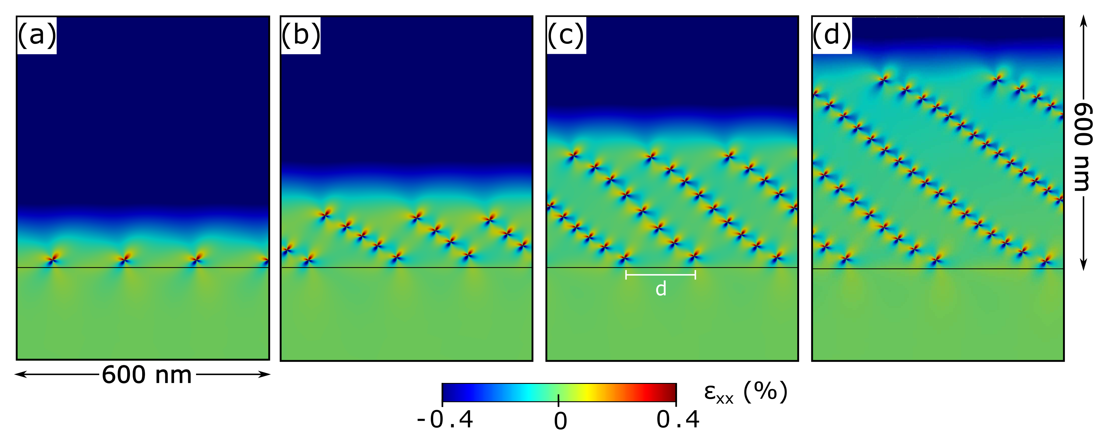
After having shown how a single dislocation introduced in a linear graded layer has an equilibrium position slightly above the interface, we continue our analysis by considering the effect of adding higher number of dislocations inside the simulation cell. In
Figure 4 we show the typical local energy minima configurations corresponding to simulations with a total number of 7 (a), 28 (b), 56 (c), and 90 (d) dislocations in a cell with a linear graded profile reaching a Ge concentration of 50% at the top of the layer. As we can observe from these results, dislocations tend to progressively relax the heteroepitaxial strain by first forming a single array of defects, all aligned at the same
y coordinate (
Figure 4a). As the number of dislocations increases, a vertical distribution of defects arises by the alignment of the dislocations into separated objects that we previously described as pileups of MDs. The angle at which the dislocations place themselves along the pileups turns out to be very close to the optimal angle found before for the interaction between two dislocations, as presented in
Figure 2e.
The spacing between the pileups, evaluated as the distance between the first dislocations of adjacent pileups as shown in
Figure 4c, however, slightly varies with increasing number of dislocations, from a minimum of
nm for the case of the single dislocation array (
Figure 4a) to a maximum of
nm as in
Figure 4d. It is worth considering, however, that these results have been evaluated consistently with the other analysis reported in this Paper for an already overcritical flat layer and for an assigned number of dislocations in the layer, without attempting to simulate a realistic growth process and its consequence on the distribution of dislocations. A more detailed analysis on the statistical nature of the results obtained by our local minimization procedure will be presented later in
Section 3.3.4. There, we will show how the proliferation of local energy-minima observed in layers with a linearly-graded concentration profile prevents the identification of the minimum-energy configuration even for an assigned set of parameters (thickness, grading rate, and number f dislocations). We will thus focus our analysis on finding the common features of the dislocation distributions observed.
3.3.3. Effect of Grading Rate
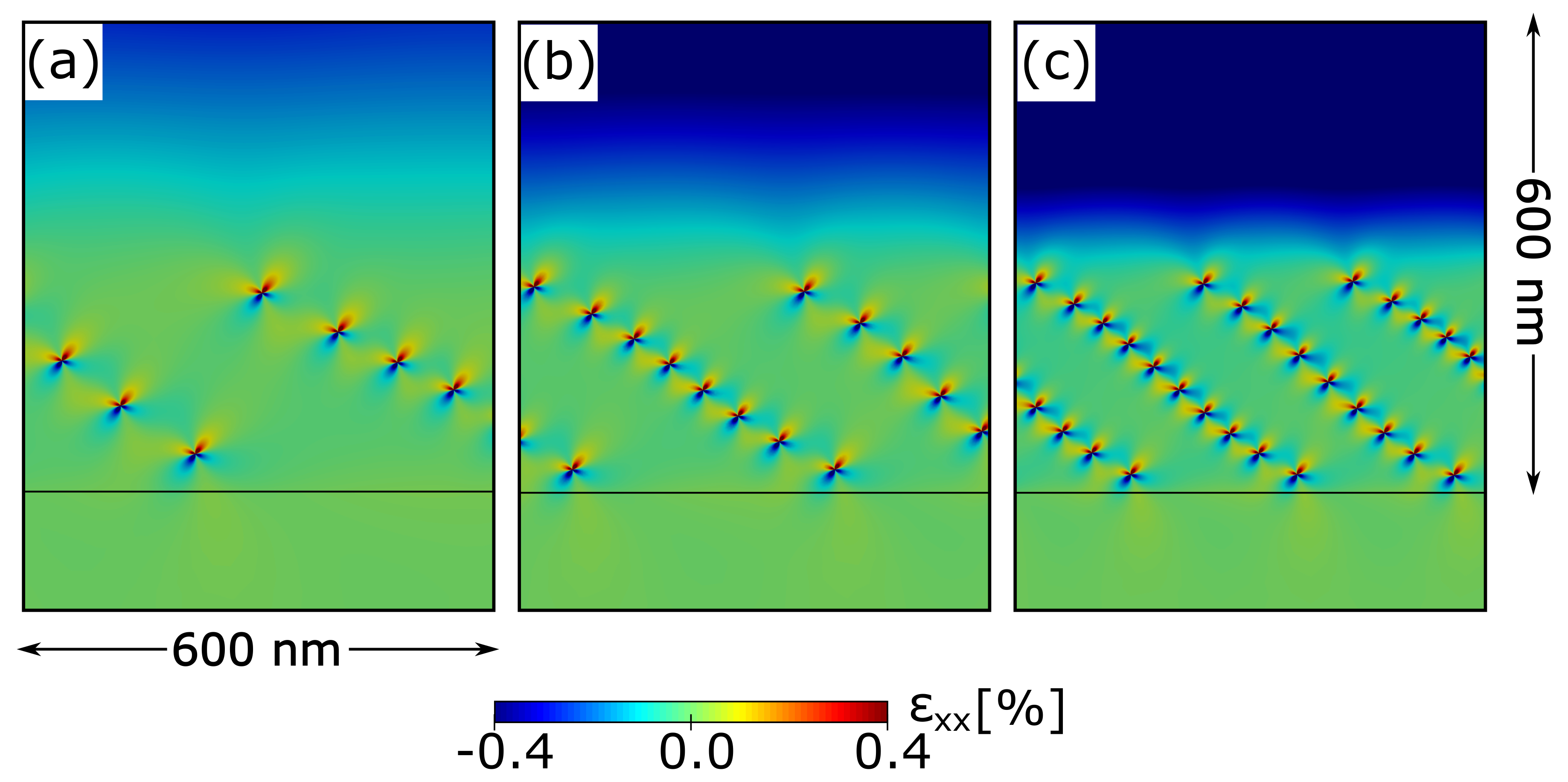
Finally, the last parameter that we can investigate in the case of a linear grading concentration profile is the Grading Rate (GR). In
Figure 5 we show the typical dislocation distributions obtained for three different values of GR. The final Ge concentrations reached at the top of the layers are, respectively,
(a),
(b), and 50 % (c), resulting in GRs in the range 20–80%
. The ratio between the GR and the number of dislocations in the simulation cell has been kept constant. The simulation reported in
Figure 5a represents the limit of the step-profiles reported in
Section 3.2 for an infinite number of layers, and thus can be seen as the final analysis of the series reported in
Figure 2. As can be seen in the image, changing the GR but keeping its ratio with the dislocation number constant results in the formation of dislocation distributions that reach the same
y coordinate for all the three cases reported in
Figure 5. This is due to the combination between the linearity in the concentration grading and the strain release as function of the dislocation number, whose ratio results in a constant value.
Finally, the effect of the change in GR can be clearly observed on the typical spacing between pileups. Indeed, this value decreases with increasing the GR. For the three cases under consideration this value is
nm in
Figure 5a,
nm in
Figure 5b, and
nm in
Figure 5c.
3.3.4. Comparison with Tersoff Model
Direct comparison between Tersoff model of Refs. [
34,
35] and our discrete dislocation coordinates is not straightforward. The analysis is further complicated by the complexity of the potential energy surface of the system under consideration. As anticipated in the analysis of the step-graded profiles of
Figure 2 a large amount of local minima can be observed starting from random initial conditions. In this Section we will focus our analysis on the minima found in the case of the graded layer presented in
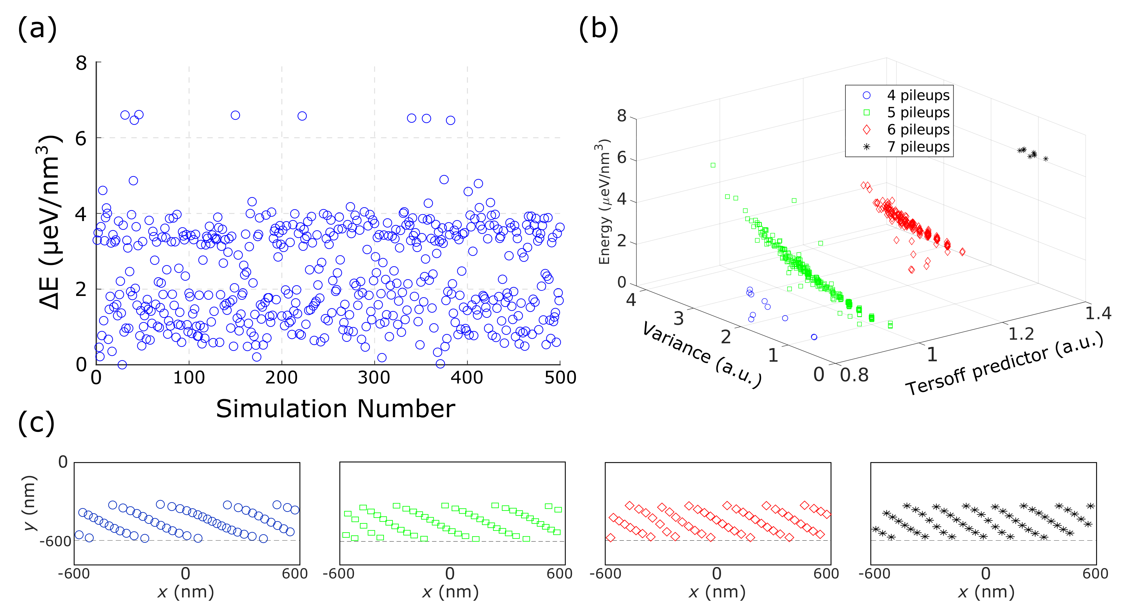
Figure 5c: a 600 nm thick film with a final Ge composition of 50%. The local minima found by running 500 independent steepest descent simulations are reported in
Figure 6a. The complexity of the dislocation configurations obtained required some further analysis before attempting their interpretation. Thus, we tried to define some appropriate descriptors to characterize the obtained local-minimum configurations.
In his mean field approach, Tersoff considered dislocations to be represented by a continuous density function
, through which the energy of a dislocated epitaxial film may be expressed as
where
is a parameter taking into account dislocation–dislocation interactions,
c is a parameter containing all relevant elastic constants,
W is the film thickness,
gives the appropriate epitaxial strain, and
the Burgers’ vector component allowing for strain release. For linearly graded systems, the dislocation density
giving the minimum energy can be proven to be in the form [
34]:
where
is the
y coordinate of the interface and
marks the beginning of the dislocation-free zone. Equation (
7) also provide results consistent with the more general picture in Ref. [
36]. In order to allow for a comparison with our results, we defined
consistently with the position of the uppermost dislocation given the grading rate and the dislocation density, which in our model is fixed at the beginning of the steepest descent procedure.
The first descriptor that we shall introduce is, therefore, a measure of the distance between the configurations obtained by our approach and the dislocation density of the Tersoff mean-field model,
. In order to obtain a dislocation density from our simulations, a kernel density estimation has been used: for each dislocation
i, a Gaussian function centered at its
position has been used to obtain a smooth distribution, with a further integration to obtain a function
depending only on the
y coordinate:
where
A is the appropriate normalization constant. The Gaussian variance
has been chosen consistently with the typical dislocations spacings, in order to avoid too much overlap between the smoothed densities. In that case, all dislocations coalesce in a single peak, hence making the density estimation useless. If
is too small, on the other hand, Dirac
-like distributions will be obtained, making the comparison impossible. In our tests, an intermediate value of
nm has proven to give the best results. We defined our descriptor
for deviations from the Tersoff-like distribution as the mean square error:
The reasons behind the choice of the error are mainly related to mathematical convenience and estimators with the same underlying idea should perform in a similar manner. Since for a linear graded profile the dislocation density extracted by the Tersoff model is constant along the vertical direction, quantify the vertical uniformity of the distribution.
The second descriptor considered was chosen after a careful analysis of the distributions of dislocations found by our steepest descent approach. Indeed, all the final configurations observed exhibit all the dislocations arranged in a certain number of pileups, like the case reported in
Figure 5c and discussed before. Thus, we exploited an automated procedure to determine the resulting number of pileups at the end of each simulation and the number of defects lying along each of those. In this way, we were able to define a second descriptor as the variance in the number of dislocations per pileups.
The energies of the local-minimum configurations found by our steepest descent algorithm plotted as a function of the predictor
defined in Equation (
9) and the variance in the number of dislocations per pileup are reported in
Figure 6b. A correlation between
and the total energy of the corresponding configuration can be observed. The trend clearly shows that the lower the value of
, the lower the energy, validating our results as being in agreement with the Tersoff model. Moreover, the plot of
Figure 6b shows also the energy dependence of the configurations with respect to the variance of the dislocation number per pileups. As can be seen, the energy is lowered by lowering the variance, meaning that uniform distribution of dislocations among the pileups are favored. An additional interesting feature may be observed in this plot: data tend to naturally cluster in subsets, each one corresponding to a different number of pileups per unit cell. The typical configurations corresponding to each of the observed subsets are reported in
Figure 6c.
3.3.5. Different Burgers Vector
In order to conclude our analysis on the linear graded concentration profiles, we considered the situation where different Burgers vectors are present within the simulation cell. As we did for the constant composition layer presented in
Section 3.1, we initialized a distribution of 56 dislocations with an equal number of defects within the two possible Burgers vector
and
, allowing for the possibility of interaction between pairs of them forming a pure-edge dislocation. In this case the results show relatively big energy dispersions depending on the starting condition as shown by the red points of
Figure 7a. The general trend is that the higher the number of dislocation pairs that reacts into a
dislocation, the lower the energy.
However, these energy dispersions, added to the complexity of the dislocation distributions in a linear graded profile, prevent any further general consideration on these distributions. In order to better investigate this case, we thus performed some additional simulations on the same system but choosing a distribution with half the number of dislocations and considering only pure-edge dislocations. The results of these calculations are reported as blue points in the same plot of
Figure 7a. The lowest energy configuration found (out of 100 simulations) corresponds to the notable case reported in
Figure 7b with all the dislocations aligned into 7 pileups of exactly 4 dislocations each one. As can be seen from the figure, in this case dislocations tend to align vertically due to the different character of the Burgers vector and thus the different symmetry of their interactions with respect to the pileups of, e.g.,
Figure 5. The result here reported, even if obtained from a local minimization procedure, can be reasonably taken as the optimal configuration for this system due to the high symmetry of the final configuration.
Since the formation of edge dislocations involves high-energy processes like the climb motion of dislocations, the observation of this minimum-energy distribution in experiments is quite difficult. Moreover, as opposed to the case of uniform composition layer discussed in
Section 3.1, typical dislocation spacing is much higher for the case under consideration, making even more complicated the path towards this configuration.
4. Conclusions
In this paper we exploited a convenient theoretical approach to determine low-energy configurations of MDs in heterolayers. Numerical simulations relied on exact (within linear elasticity theory) analytical expressions for the non-singular, periodic stress field of dislocations near free surfaces. We are not aware of previous publications where such expressions were derived and used.
After having validated our approach against some well-known results regarding dislocation distributions in uniform composition layers, we focused our attention on the linear graded profile. With our approach we were able to overcome the typical limitations of the mean-field approaches, like the one proposed by Tersoff [
34], by the ability to retain information on the position of individual defects. The results found for low-energy configurations of equal 60
dislocations were analyzed in depth. We were thus able to demonstrate that the common feature of such dislocation distributions is the alignment of the defects along structures commonly referred as pileups of MDs. Furthermore, the driving forces leading to this behavior were elucidated by the analysis of the step-graded profiles, explaining how the dislocation–dislocation interactions influence the observed arrangements. Interestingly, such low-energy profiles closely resemble the output of a well-known kinetic process, i.e., multiplication of dislocations triggered by Frank–Read or modified Frank–Read sources [
37]. Such multiplication mechanism, indeed, produces injection of a certain number of dislocations with the same Burgers vector aligned along a specific glide plane. Here, we have shown that there exists also a thermodynamic driving force for the formation of analogous dislocation distributions.
Finally, when considering distributions with two possible Burgers vectors, we demonstrated the tendency towards the reaction of dislocations in order to form pure-edge defects. When all of them were able to coalesce into edge dislocations, the distributions were characterized by defects aligned into vertical pileups. A configuration with perfect ordering of the dislocations was found, possibly representing the lowest-energy configuration in this system. However, our un-constrained minimization procedure can produce results that are not easily replicable in experiments due to the presence of high-energy activation processes. Nevertheless, the result here obtained can be a suitable starting point for the interpretation of experimental observations of complex MDs distributions in graded layers.


