Article

Parameter Estimation of the Stochastic Primary Nucleation Kinetics by Stochastic Integrals Using Focused-Beam Reflectance Measurements

Department of Applied Chemistry, Waseda University, Okubo 3-4-1, Shinjuku, Tokyo 169-8555, Japan
*
Author to whom correspondence should be addressed.
Crystals 2020, 10(5), 380; https://doi.org/10.3390/cryst10050380
Submission received: 27 April 2020 / Revised: 1 May 2020 / Accepted: 4 May 2020 / Published: 7 May 2020
(This article belongs to the Special Issue Crystal Nucleation and Growth Kinetics)

Abstract

:
The kinetic parameters of stochastic primary nucleation were estimated for the batch-cooling crystallization of L-arginine. It is difficult for process analytical tools to detect the first nucleus. In this study, the latent period for the total number of crystals to be increased to a predetermined threshold was repeatedly measured with focused-beam reflectance measurements. Consequently, the latent periods were different in each measurement due to the stochastic behavior of both primary and secondary nucleation. Therefore, at first, the distribution of the latent periods was estimated by a Monte Carlo simulation for some combinations of the kinetic parameters of primary nucleation. In the simulation, stochastic integrals of the population and mass balance equations were solved. Then, the parameters of the distribution of latent periods were estimated and correlated with the kinetic parameters of primary nucleation. The resulting correlation was represented by a mapping. Finally, the parameters of the actual distribution were input into the inverse mapping, and the kinetic parameters were estimated as the outputs. The estimated kinetic parameters were validated using statistical techniques, which implied that the observed distribution function of the latent periods for the thresholds used in the estimation coincided reasonably with the simulated one based on the estimated parameters.

Graphical Abstract

1. Introduction

The nucleation and growth kinetics of crystallization strongly affects the crystal quality, especially the crystal size distribution (CSD) [1,2,3] and, hence, needs to be described in crystallization processes. However, nucleation occurs stochastically rather than deterministically [4,5,6], which may make it difficult to control the crystallization processes. This stochastic nature of nucleation has been reported to be caused by a rarity of the nucleation event [7,8]. Nucleation can be classified into primary nucleation and secondary nucleation. When the system adequately contains the crystals, secondary nucleation occurs so frequently that it can be regarded as deterministic [9,10]. On the other hand, primary nucleation is often regarded as the stochastic process, and this stochastic behavior has been studied by many researchers [11,12,13].
Some difficulties arise when the primary nucleation kinetics is investigated in the unseeded batch-cooling crystallizer by using process analytical tools (PATs). First, it is impossible for many PATs to detect the very first nucleus in a large crystallizer [14]. The instruments can finally detect nucleation when the solution comes to suspend a certain number of crystals, which may include grown secondary nuclei. Secondly, the ends of the latent periods, when the PATs detect a predetermined state of the solution, can differ from one another in several measurements due to the stochastic behavior of nucleation. In order to overcome these difficulties, the population and mass balance equations, including stochastic primary nucleation, needs to be solved [9]. These differential equations include the terms that are the stochastic processes, and hence, the solutions of the equations are also the stochastic processes. The distribution of the latent periods may be reproduced by the stochastic integrals.
In addition, several difficulties in the stochastic integrals remain unsolved yet. At first, the stochastic behavior of secondary nucleation was ignored in many reports on the stochastic integrals of the population balance equations. However, secondary nucleation may not occur frequently in the early stage of unseeded or partially seeded crystallization and can behave in a stochastic manner. In fact, the stochastic behavior of secondary nucleation was studied in [15,16]. Then, many algorithms developed for solving the stochastic integrals specialized in stochastic primary nucleation. It might be difficult for these algorithms to handle other stochastic processes such as stochastic secondary nucleation.
This work aims to estimate the kinetic parameters of stochastic primary nucleation in cooling crystallization of L-arginine (Arg). First, the kinetic parameters of secondary nucleation and growth are determined by preliminary experiments based on our previous studies [17,18]. Secondly, the parameters of the distribution of latent periods for the total number of crystals to be increased to a predetermined threshold are estimated and correlated with the kinetic parameters of stochastic primary nucleation by means of a Monte Carlo simulation. In this simulation, the stochastic integrals of the population and mass balance equations are repeatedly solved with the method of moments. A reasonable approximation is introduced into the stochastic integrals, which enables stochastic secondary nucleation to be considered. The parameters of the distribution are estimated at several points in the space of the kinetic parameters, and the resulting correlation is represented by a mapping. Thirdly, the latent period is repeatedly measured with focused beam reflectance measurement (FBRM) and Fourier transform infrared-attenuated total reflection spectroscopy (FT-IR-ATR), from which the actual distribution of the latent periods is obtained. Fourthly, the parameters of the obtained distribution of the latent periods are input into the inverse mapping, and the kinetic parameters of stochastic primary nucleation are estimated as the outputs. Finally, the estimated kinetic parameters and the consideration to stochastic secondary nucleation are validated using the stochastic integrals and the statistical techniques.

2. Materials and Methods

2.1. Substances and Devices

An aqueous solution of L(+)-arginine (C6H14N4O2, abbreviated to Arg) was utilized as a target substance in this study. Arg (>98.0%) was purchased from FUJIFILM Wako Pure Chemical Corporation (Osaka, Japan). Arg is a basic amino acid, which nourishing tonics often contain, and there are few studies on the crystallization of Arg. In our previous work [17,18], the characteristics of growth and secondary nucleation for the crystallization of Arg were investigated as a typical hydrophilic amino acid, and hence, Arg was selected also in this study. The physical properties of the substance are listed in Table 1.
The in-line measurements of the solution temperature, the chord length distribution (CLD), and the IR spectrum were conducted simultaneously. The solution temperature was measured with a platinum electrode (model CENTER376 made by Sato Shoji Corporation, Tokyo, Japan) and was controlled in a jacketed beaker with a programmable controller (model AD-4820, made by A&D Company Limited, Tokyo, Japan).
The CLD was measured with focused beam reflectance measurement (FBRM, made by Mettler Toledo International Inc., Columbus, OH, USA). The FBRM technique is often applied to obtain the size distribution [19,20,21]. However, the CLD obtained with FBRM is different from CSD, and hence, the CLD needs to be converted into the CSD [22,23]. In our previous work [18,24], the method for the conversion was investigated for the Arg crystals and is represented as follows:
N CLD = S   N CSD ,
where S is mapping matrix, and N is frequency-length or frequency-size distribution. Each element of S corresponds with the probability that a crystal with a certain size will be measured as a certain chord length [18]. In this study, S was computed with a Monte Carlo analysis in MATLAB (version R2019a made by The MathWorks, Inc., Natick, MA, USA) [25,26], in which crystals with a predetermined shape were rotated and translated randomly [24,27]. Settings of the Monte Carlo analysis and the instruments for FBRM are listed in Table 2. A number-size distribution was deduced from the frequency-size distribution and the total mass of crystals based on the mass balance.
The IR spectrum was measured with Fourier transform infrared-attenuated total reflection spectroscopy (FT-IR-ATR, made by Mettler Toledo International Inc., Columbus, OH, USA) and was utilized for obtaining the Arg concentration. The peak intensity of the FT-IR-ATR has been reported to be affected by the solution temperature [28,29]. The calibration equation used in this study is represented as follows:
A = α IR C + β IR T + γ IR ,
where A is peak area to the two-point baseline; C is the concentration or mass of solute per unit mass of solvent; T is the Celsius temperature of the solution; and α, β, and γ are regression coefficients. The regression coefficients were estimated in each measurement. An example of the estimation of the regression coefficients is illustrated in Figure 1, and the measurement conditions of the FT-IR-ATR are listed in Table 3. In Figure 1, the dotted line of concentration denotes that the concentration was unknown. The range of data marked by the gray arrows was utilized to obtain the calibration equation of A = 6.58 C − 0.00696 T + 0.471.

2.2. Experimental Procedure

A saturated amount of Arg anhydrate was dissolved in 300 mL of water at an initial temperature higher than the saturated temperature. Then, the solution was linearly cooled down to the final temperature and stirred with a four-blade agitator (φ40) at the rotation speed of 400 rpm. During cooling in the preliminary experiments, sieved seed crystals with the size range of 44–74 μm were added when the solution temperature reached the saturated temperature. After cooling, the solution temperature was kept at the final temperature for a while. The conditions of the preliminary experiments and the main experiments are listed in Table 4. The preliminary experiments were performed for the estimation of the secondary nucleation and growth kinetics, and the main ones for the estimation of the primary nucleation kinetics.

2.3. Mathematical Model

Growth is regarded as deterministic, and this rate is represented as follows [30,31]:
G = k g ( S 1 ) g ,
where kg and g are the growth rate coefficient and order, respectively, and S is the supersaturation ratio. Saturation and supersaturation are expressed as follows:
C sat = f sat ( T ) = α sat T 2 + β sat T + γ sat ,
T sat = f sat 1 ( C ) ,
S = C C sat ,
where Csat is the solubility at temperature T, Tsat is the saturation temperature at concentration C, the subscript “sat” denotes saturation, and regression coefficients of the solubility curve are also listed in Table 1. Primary nucleation and secondary nucleation are regarded as stochastic, and expected values of these rates are represented as follows, respectively [31,32,33]:
B 1 = E [ B 1 * ] = k b 1 exp [ b 1 ( ln S ) 2 ] ,
B 2 = E [ B 2 * ] = k b 2 ( T sat T ) b 2 μ 3 ,
where kb1 and b1 are the primary nucleation rate coefficient and order, kb2 and b2 are the secondary nucleation rate coefficient and order, the superscript “*” emphasizes that the value is a stochastic variable, and μ3 is the third moment of the CSD. The i-th moment of the CSD is defined as follows:
μ i = 0 n L i d L .
Here, n is the population density or crystal number per unit mass of solvent per unit crystal size, depending on time t and crystal size L. The total nucleation rate and its expectations are represented as follows, respectively, due to the linearity of the expectations:
B * = B 1 * + B 2 * ,
B = B 1 + B 2 .
Then, the probability that the number of crystals newly nucleated from t to t + τ will equal k is denoted as follows:
P ( τ , t ; k ) = Pr { t t + τ W s B * d τ = k } ,
where the concentration begins to exceed the solubility at t = 0, W is the mass, and the subscript “s” denotes the solvent. At most one nucleus is assumed to appear during an infinitesimal time, and hence, the following equation is established:
{ τ P ( τ , t ; k ) = W s B P ( τ , t ; k ) + W s B P ( τ , t ; k 1 )   ( k ) τ P ( τ , t ; 0 ) = W s B P ( τ , t ; 0 ) .
The following equations are derived by solving Equation (13) [9,14]:
P ( τ , t ; k ) = ( t t + τ W s B d τ ) k k ! exp [ t t + τ W s B d τ ] ,
t t + τ W s B * d τ Po [ t t + τ W s B d τ ] ,
where Equation (15) means that the number of crystals newly nucleated from t to t + τ follows a Poisson distribution with the parameter in the right side. Here, τ is substituted by a reasonably short time Δt to derive approximately the following equations:
P ( Δ t , t ; k ) Pr { W s ( t ) B * ( t ) Δ t = k } ,
B * ( t ) Po [ W s ( t ) B ( t ) Δ t ] W s ( t ) Δ t ,
where Δt should be so short a time that the change in the expectation of the nucleation rate and the increase in the crystal size can be ignored during Δt. In this study, Δt was determined as follows: At first, the deterministic population and mass balance equations were solved with a variable step solver. In solving the equations, the solver based on the Runge-Kutta (4,5) formula was utilized in MATLAB [34,35]. Then, the shortest time step that had a predetermined acceptable error was detected when the change in the solution of the equations was sharpest, and this time step was adopted as Δt. Finally, the stochastic population and mass balance equations were solved with the step of the solver fixed to Δt, where random numbers from the Poisson distribution were generated in MATLAB [36]. The stochastic population and mass balance equations are represented as follows [37,38]:
t ( W s n ) + G L ( W s n ) = W s B * δ ( L L 0 ) ,
t W h = R h t W a = R h R h 1 t W s = ρ c k v t ( W s μ 3 ) = 3 ρ c k v G W s μ 2 + ρ c k v W s B * L 0 3 ,
where δ is the Dirac delta function, the subscripts “h” and “a” denote the hydrated crystal and anhydrated solute, and all solutions of these equations are also the stochastic processes due to stochastic nucleation. The method of moments is utilized to derive the following equation [38]:
{ t ( W s μ i ) = i G W s μ i 1 + W s B * L 0 i   ( i = 1 , 2 , 3 ) t ( W s μ 0 ) = W s B * .

2.4. Parameter Estimation

In the preliminary experiments, seed crystals are assumed to have been added so sufficiently that secondary nucleation could be regarded as deterministic and the primary nucleation rate to have been negligible. First, in order to estimate the kinetic parameters of secondary nucleation, the data of so-called metastable zone widths were acquired, and the regression analysis was carried out based on the following approximate equation:
log ( Δ T m ) 1 b 2 + 1 log ( R ln r ) + 1 b 2 + 1 log ( b 2 + 1 ) μ 0 , seed k b 2 μ 3 , seed = α B 2 log ( R ln r ) + β B 2 .
Here, R is the cooling rate, the subscript “seed” denotes the seed crystals, and ΔTm and r are defined as follows:
Δ T m = T sat | t = 0 T | μ 0 = μ 0 , m ,
r = μ 0 , m μ 0 , seed ,
where the subscript “m” means that the number of crystals reaches a predetermined threshold in this study. Equation (21) can be derived from Equation (20) as follows [17]: First, it is assumed from t = 0 to the threshold that C and Ws are constant, μ3 is proportional to μ0, and that μ0,seed is negligibly small compared with rμ0,seed. Secondly, B2 is substituted for B* into Equation (20) at i = 0, and this equation is integrated from t = 0 to the threshold. Thirdly, the same equation is integrated with μ3 fixed to the average value. Fourthly, the derivation of the second step is substituted into that of the third step, and the relation between the μ3,seed and the averaged μ3 is derived. Finally, the derivation of the fourth step is substituted into Equation (20) at i = 0, and this equation is integrated with t substituted by ΔT/R to derive Equation (21). Here, ΔT is a decrease in the solution temperature. Several thresholds can be set in one measurement only if the errors between the initial concentration and actual ones satisfy the following restriction:
T sat | t = 0 T sat | μ 0 = μ 0 , m Δ T m < ε ,
where ε was set to 0.2 in this study. Equation (24) should be satisfied, because the decrease in concentration is ignored in Equation (21). An example of the data acquisition of metastable zone widths is illustrated in Figure 2. At the points marked by the circles, the errors satisfied Equation (24), and the data were accepted and added to the dataset. The μ0,seed was obtained as the average value in the preliminary measurements.
Secondly, in order to estimate the kinetic parameters of growth, the growth rates were approximately computed by the following equation derived from Equation (19):
G 1 3 ρ c k v W s μ 2 Δ W h Δ t ,
where Δt is reasonably small measuring interval. The data of G were acquired, and the regression analysis was carried out based on the following equation:
log G = g log ( S 1 ) + log k g = α G log ( S 1 ) + β G .
Several datapoints can be obtained in one measurement only if the errors between the actual changes in the mass of crystals and contributions of growth satisfy the following restriction:
( ρ c k v W s B 2 L 1 3 ) / ( Δ W h Δ t ) < ε ,
where the numerator in the left side is the contribution of the secondary nucleation, and ε was set to 0.2 in this study. Equation (27) should be satisfied, because the contribution of the secondary nucleation is ignored in Equation (25). In the measuring interval of Δt, the nuclei may grow to have an average size of L1, which should be represented as follows:
L 1 3 = ( L 0 L 0 + G Δ t L 3 d L ) / ( L 0 L 0 + G Δ t d L ) .
Thirdly, in order to estimate the kinetic parameters of stochastic primary nucleation, the data of the so-called latent periods were acquired from the main experiments. Several thresholds can be set in one measurement, and the latent period for the j’-th threshold satisfies the following equation:
( W s μ 0 ) m , j = 0 t m , j * W s B * d t ,
where the subscript “m” means that the total number of crystals reaches a predetermined threshold, and the latent period is also a stochastic variable. An example of the data acquisition of latent periods is illustrated in Figure 3, where the maximum number of crystals was obtained as the approximate average value in the main measurements.
The acquired data gave the parameters of the distribution of the latent periods, such as a mean and a standard deviation. On the other hand, a certain combination of the kinetic parameters of the stochastic primary nucleation may give the corresponding parameters of the distribution of latent periods by solving Equations (19) and (20) repeatedly. In this study, five hundred latent periods were simulated for each threshold and for each combination. Then, the parameters of the distribution were estimated at several points in the space of the kinetic parameters, and the resulting correlation was represented by a mapping as follows:
θ d = F ( θ B 1 ) = [ θ d , 1 θ d , j ] = [ μ t m , 1 * σ t m , 1 * μ t m , j * σ t m , j * ] ,
where j is the number of thresholds, θ is the parameter vector, F is the mapping, which contains interpolants computed in MATLAB [39], the subscripts “d” and “B1” denote the distribution and kinetics of the primary nucleation, μ and σ are the mean and standard deviation, and θB1 was defined as follows in this study:
θ B 1 = [ log k b 1 b 1 ] .
Conversely, the parameters of the distribution of the observed latent periods are input into the inverse mapping to estimate the kinetic parameters of the stochastic primary nucleation as follows:
θ ^ B 1 = F 1 ( θ ^ d ) arg min θ B 1 j { F j ( θ B 1 ) θ ^ d , j θ ^ d , j } 2 ,
where that emphasizes that the value is an unbiased estimator obtained from actual measurements, and the minimization was conducted with the trust-region-reflective algorithm in MATLAB [40,41,42].

2.5. Validation

At first, the estimated parameters were substituted into the rate equations, and latent periods were simulated five hundred times. Then, the simulated cumulative distribution function of the latent periods was compared to the observed one with 99% confidence bounds. For calculating the confidence bounds, the Kaplan-Meier method was utilized as follows [43]:
Pr * ( t m , obsd * t m ) ~ N [ Pr ( t m , obsd * t m ) , V [ Pr * ( t m , obsd * > t m ) ] ] ,
where the left side is the probability that the observed latent period will take a value less than or equal to a certain latent period, and this probability in itself is assumed to follow a normal distribution with the parameters in the right side. Here, the subscript “obsd” denotes an observed value, N is the normal distribution, and V is the variance, which is estimated as follows [43]:
V [ Pr * ( t m , obsd * > t m ) ] = { Pr ( t m , obsd * > t m ) } 2 t l < t m 1 ν l ( ν l 1 ) .
Here, νl’ is the number of samples within their own latent period at time tl’ when some sample finishes its latent period, and it is assumed that no two samples finish their latent period at the same time. In addition, the test statistics of the two-sample Kolmogorov-Smirnov test were computed to obtain the p-value. The test statistic is defined as follows:
D = max t m ( | Pr ( t m , simd * t m ) Pr ( t m , obsd * t m ) | ) ,
where the subscript “simd” denotes a simulated value. The p-value is approximately computed with the following equation [44,45]:
Pr ( l D > x ) 1 ϑ ( 1 2 ; 2 1 π x 2 ) ,
where ϑ is the Jacobi theta function, and l are defined as follows:
l = l s i m d   ·   l o b s d l s i m d + l o b s d ,
where lsimd or lobsd is the total number of samples, and l was about 23.8 in this study. The p-value is computed by substituting the test statistic for x. The small p-value implies the difference between the simulated distribution and the observed one. Finally, the deterministic secondary nucleation rate was substituted for the stochastic one into the population and mass balance equations, and the validation was carried out in the same way.

3. Results and Discussion

3.1. Parameter Estimation
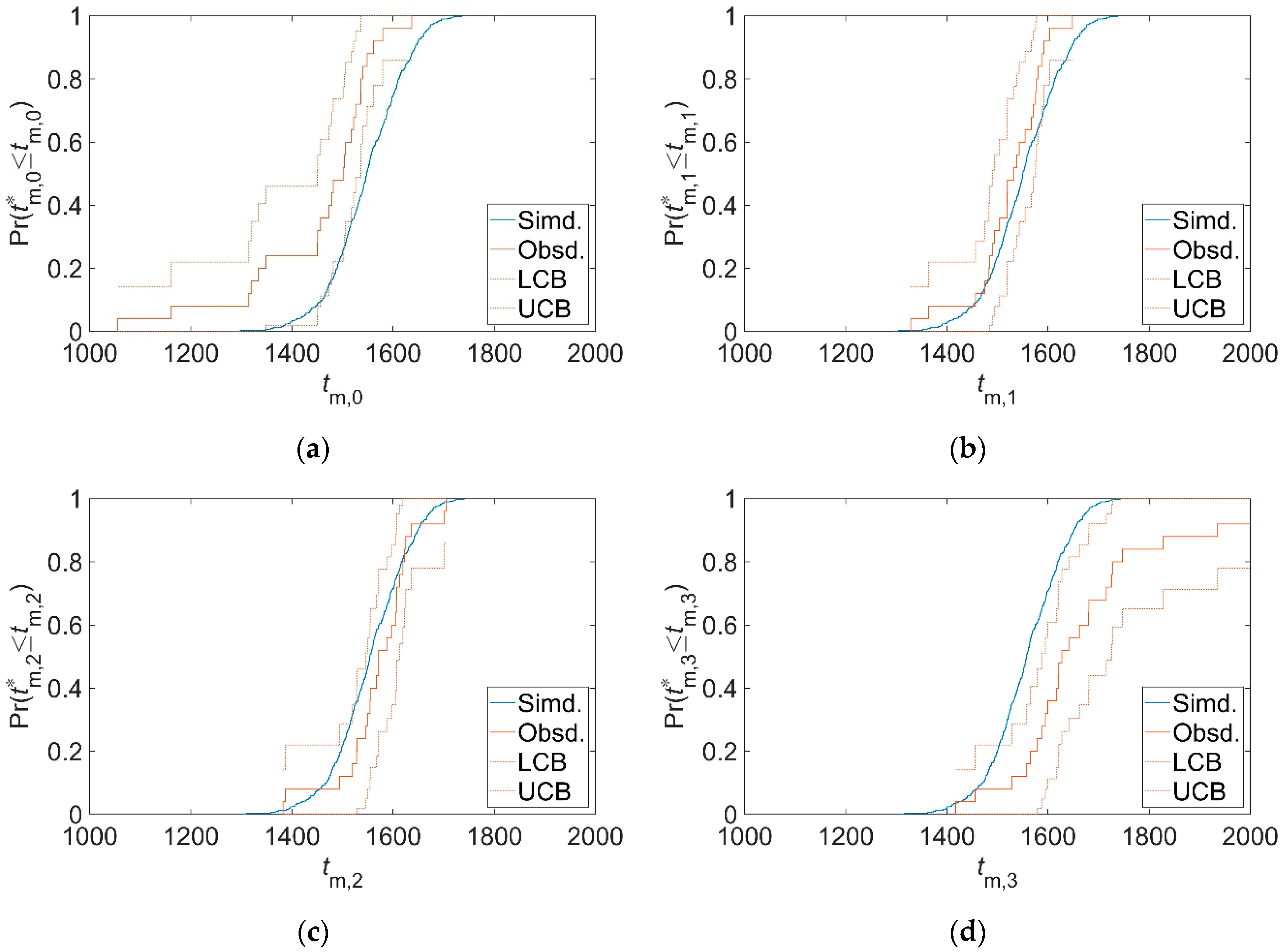
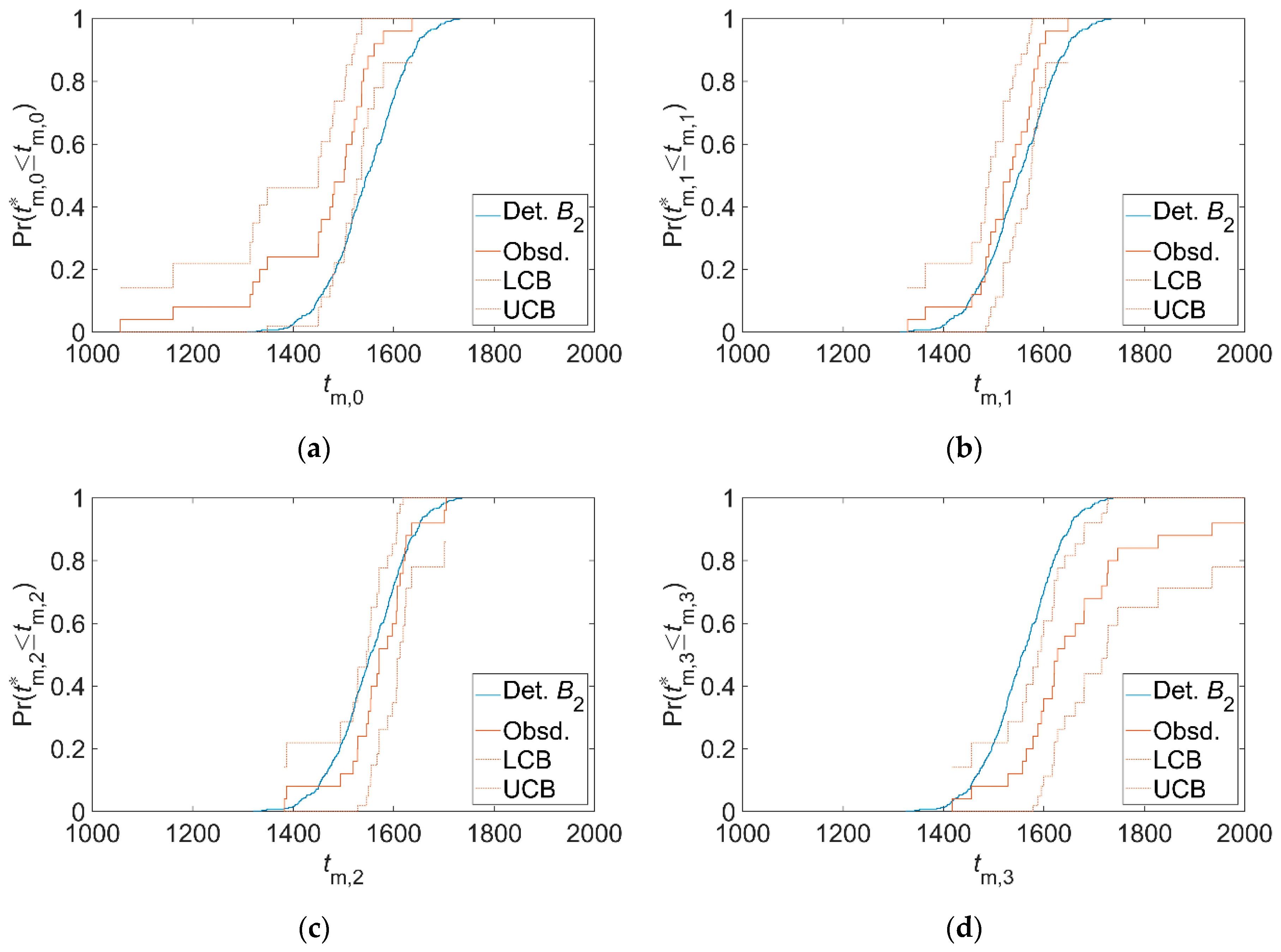
In the preliminary experiments, the kinetic parameters of the secondary nucleation and growth were estimated based on the regression analyses expressed in Equations (21) and (26). The resulting regression lines are illustrated in Figure 4 and Figure 5, respectively, and the estimated parameters are listed in Table 5. In Figure 4, the unit of R is K/s.
In the main experiments, at first, the latent periods for the four thresholds were measured twenty-five times, and the mean and the standard deviations of the latent periods were estimated for each threshold. The means and the standard deviations are listed in Table 6. At j’ = 0 in Table 6, the standard deviation is large, which is attributed to a low sensitivity of the instruments for the small number of crystals. Moreover, at j’ = 3, the standard deviation is also large, which might be attributed to the agglomeration, breakage, and heat of crystallization. Therefore, the data for these thresholds were rejected in this study.
Then, the means and the standard deviations for the accepted thresholds were estimated at several points in the space of the kinetic parameters, and the resulting correlation was represented by a mapping. The mapping is outlined in Figure 6. In Figure 6, the parameters of the distribution were estimated at 7 × 5 points in the space of the kinetic parameters, and the bold lines correspond to the unbiased estimators obtained from the actual measurements. In short, the resulting kinetic parameters should be reasonably close to all the bold lines. The estimation of the kinetic parameters of the stochastic primary nucleation is outlined in Figure 7, and the estimated parameters are also listed in Table 5. When the dimensions of the parameters of the distribution are less than that of the kinetics, the estimators are undetermined, as is marked by the lines in Figure 7. When they are equal, the estimators are determined uniquely, as is marked by the circle and the square. When those of the distribution are more than that of the kinetics, the estimators are overdetermined, and approximate solutions are obtained, as is marked by the triangle.
In this study, the kinetic parameters were defined by Equation (31) and the parameters of the distribution by Equation (30). These parameters can be changed, removed, or added. For example, in order to add the activation energy of the primary nucleation to the kinetic parameters, other parameters of the distribution with a low degree of multicollinearity should be added to the current parameters of the distribution, such as the ones obtained under the operating conditions with other cooling rates or with other initial temperatures. In addition, the confidence intervals of the kinetic parameters can be estimated based on those of the parameters of the distribution.

3.2. Validation

The simulated and observed cumulative distribution functions of latent periods are illustrated in Figure 8, where the secondary nucleation is regarded as stochastic in the simulations, and in Figure 9, where the secondary nucleation as stochastic. In Figure 8 and Figure 9, the LCB and UCB are the lower and upper confidence bounds of an observed function, respectively. In Figure 8b,c, the simulated and observed ones are assumed to coincide reasonably, which might be attributed to the trueness of the estimated parameters. On the other hand, In Figure 8a,d, the differences between the simulated ones and the observed ones are significant, which might be attributed to the large standard deviations mentioned in the previous subsection. Moreover, there is no significant difference between Figure 8 and Figure 9. The p-values of the two-sample Kolmogorov-Smirnov test are also listed in Table 6, which implies that the ignorance of the stochastic behavior of the secondary nucleation makes the larger difference between the simulated distribution and the observed one for the accepted thresholds.
In this study, the agglomeration, breakage, and the heat of crystallization were not considered in the mathematical model. However, the agglomeration and breakage were reported to be significant at a high magma density [46,47], and the heat of the crystallization is assumed to have greatly affected the latent period at j’ = 3 (10% of max.) in Figure 3. In order to improve the accuracy of the estimation, these factors should be added to the mathematical model in future works.

4. Conclusions

The kinetic parameters of the stochastic primary nucleation were estimated for Arg crystallization. First, the kinetic parameters of the secondary nucleation and growth were determined by preliminary experiments, where the secondary nucleation and growth were regarded as deterministic. Secondly, in order to estimate the remaining kinetic parameters of the primary nucleation, the mean and standard deviation of the latent periods for the total number of crystals to be increased to a predetermined threshold were estimated and correlated with the kinetic parameters of the primary nucleation by means of a Monte Carlo simulation, where the primary nucleation and secondary nucleation were regarded as stochastic. Thirdly, in order to obtain the actual distribution of the latent periods, the latent period was repeatedly measured with FBRM and FT-IR-ATR. Fourthly, the means and the standard deviations of the obtained latent periods for the two thresholds were input into the inverse mapping, and the kinetic parameters of the stochastic primary nucleation were estimated as the outputs. Fifth, the estimated kinetic parameters were validated using the stochastic integrals and the cumulative distribution functions. Consequently, the simulated and observed functions were assumed to coincide reasonably for the two thresholds used in the estimation. However, the differences between the simulated ones and the observed ones were significant for the thresholds that were not used in the estimation, which might be attributed to the agglomeration, breakage, heat of crystallization, and a low sensitivity of the instruments for the small number of crystals. Finally, the considerations to stochastic secondary nucleation were validated using the stochastic integrals and the two-sample Kolmogorov-Smirnov test. The resulting p-values calculated from stochastic secondary nucleation for the two thresholds used in the estimation were relatively large compared to those calculated from deterministic secondary nucleation, which implied that the ignorance of the stochastic behavior of secondary nucleation made the larger difference between the simulated distribution and the observed one.
In this study, the primary nucleation coefficient and order were estimated in the main experiments. These parameters can be changed, removed, or added, and then, the changed parameters can be estimated in the same way as in this work. For example, the activation energy of the primary nucleation will be added to the kinetic parameters and estimated in a future work. Moreover, in order to improve the accuracy of the estimation, the agglomeration, breakage, and the heat of crystallization should be added to the mathematical model in a future work.

Author Contributions

Conceptualization, J.U. and I.H.; methodology, J.U.; software, J.U.; validation, J.U. and I.H.; formal analysis, J.U.; investigation, J.U.; resources, J.U.; data curation, J.U.; writing—original draft preparation, J.U.; writing—review and editing, I.H.; visualization, J.U.; supervision, I.H.; project administration, I.H.; and funding acquisition, I.H. All authors have read and agreed to the published version of the manuscript.

Funding

This research received no external funding.

Acknowledgments

The authors would like to acknowledge the technical support and the provisions of the devises from Mettler-Toledo K.K. BU AutoChem.

Conflicts of Interest

The authors declare no conflict of interest.

References

  1. Weng, J.; Huang, Y.; Hao, D.; Ji, Y. Recent advances of pharmaceutical crystallization theories. Chin. J. Chem. Eng. in press. [CrossRef]
  2. El-Zhry El-Yafi, A.K.; El-Zein, H. Technical crystallization for application in pharmaceutical material engineering: Review article. Asian J. Pharm. Sci. (Amsterdam, Neth.) 2014, 10, 283–291. [Google Scholar] [CrossRef] [Green Version]
  3. Tung, H.-H. Industrial perspectives of pharmaceutical crystallization. Org. Process Res. Dev. 2013, 17, 445–454. [Google Scholar] [CrossRef]
  4. Artusio, F.; Pisano, R. Surface-induced crystallization of pharmaceuticals and biopharmaceuticals: A review. Int. J. Pharm. (Amsterdam, Neth.) 2018, 547, 190–208. [Google Scholar] [CrossRef]
  5. Sleutel, M.; Van Driessche, A.E.S. Nucleation of protein crystals-a nanoscopic perspective. Nanoscale 2018, 10, 12256–12267. [Google Scholar] [CrossRef]
  6. Sear, R. What do crystals nucleate on? What is the microscopic mechanism? How can we model nucleation? MRS Bull. 2016, 41, 363–368. [Google Scholar] [CrossRef]
  7. Kulkarni, S.A.; Kadam, S.S.; Meekes, H.; Stankiewicz, A.I.; Ter Horst, J.H. Crystal nucleation kinetics from induction times and metastable zone widths. Cryst. Growth Des. 2013, 13, 2435–2440. [Google Scholar] [CrossRef]
  8. Jiang, S.; Ter Horst, J.H. Crystal nucleation rates from probability distributions of induction times. Cryst. Growth Des. 2011, 11, 256–261. [Google Scholar] [CrossRef]
  9. Maggioni, G.M.; Mazzotti, M. A Stochastic Population Balance Equation Model for Nucleation and Growth of Crystals with Multiple Polymorphs. Cryst. Growth Des. 2019, 19, 4698–4709. [Google Scholar] [CrossRef]
  10. Maggioni, G.M.; Bezinge, L.; Mazzotti, M. Stochastic nucleation of polymorphs: Experimental evidence and mathematical modeling. Cryst. Growth Des. 2017, 17, 6703–6711. [Google Scholar] [CrossRef]
  11. Kadam, S.S.; Kulkarni, S.A.; Coloma Ribera, R.; Stankiewicz, A.I.; ter Horst, J.H.; Kramer, H.J.M. A new view on the metastable zone width during cooling crystallization. Chem. Eng. Sci. 2012, 72, 10–19. [Google Scholar] [CrossRef]
  12. Kubota, N. An attempt to explain the waiting time distribution for primary nucleation of potassium sulphate from aqueous solution by a stochastic model. J. Cryst. Growth 1983, 62, 161–166. [Google Scholar] [CrossRef]
  13. Thijssen, H.A.C.; Vorstman, M.A.G.; Roels, J.A. Heterogeneous primary nucleation of ice in water and aqueous solutions. J. Cryst. Growth 1968, 3–4, 355–359. [Google Scholar] [CrossRef]
  14. Kubota, N. Analysis of the effect of volume on induction time and metastable zone width using a stochastic model. J. Cryst. Growth 2015, 418, 15–24. [Google Scholar] [CrossRef]
  15. Kubota, N.; Kubota, K. Secondary nucleation of magnesium sulphate from single seed crystal by fluid shear in agitated supersaturated aqueous solution. J. Cryst. Growth 1986, 76, 69–74. [Google Scholar] [CrossRef]
  16. Kubota, N.; Karasawa, H.; Kawakami, T. On estimation of critical supercooling from waiting times measured at constant supercooling — A secondary nucleation from a single seed crystal of potash alum suspended in agitated solution. J. Chem. Eng. Jpn. 1978, 11, 290–295. [Google Scholar] [CrossRef] [Green Version]
  17. Unno, J.; Kawase, H.; Kaneshige, R.; Hirasawa, I. Estimation of Kinetics for Batch Cooling Crystallization by Focused-Beam Reflectance Measurements. Chem. Eng. Technol. 2019, 42, 1428–1434. [Google Scholar] [CrossRef]
  18. Unno, J.; Umeda, R.; Hirasawa, I. Computing Crystal Size Distribution by Focused-Beam Reflectance Measurement when Aspect Ratio Varies. Chem. Eng. Technol. 2018, 41, 1147–1151. [Google Scholar] [CrossRef]
  19. Trampuž, M.; Teslić, D.; Likozar, B. Crystallization of fesoterodine fumarate active pharmaceutical ingredient: Modelling of thermodynamic equilibrium, nucleation, growth, agglomeration and dissolution kinetics and temperature cycling. Chem. Eng. Sci. 2019, 201, 97–111. [Google Scholar] [CrossRef]
  20. Pandit, A.; Katkar, V.; Ranade, V.; Bhambure, R. Real-Time Monitoring of Biopharmaceutical Crystallization: Chord Length Distribution to Crystal Size Distribution for Lysozyme, rHu Insulin, and Vitamin B12. Ind. Eng. Chem. Res. 2019, 58, 7607–7619. [Google Scholar] [CrossRef]
  21. Kim, W.-S.; Koo, K.-K. Crystallization of Azilsartan with Acidification of Azilsartan Disodium Salt. Cryst. Growth Des. 2019, 19, 1797–1804. [Google Scholar] [CrossRef]
  22. Ruf, A.; Worlitschek, J.; Mazzotti, M. Modeling and experimental analysis of PSD measurements through FBRM. Part. Part. Syst. Charact. 2000, 17, 167–179. [Google Scholar] [CrossRef]
  23. Kail, N.; Briesen, H.; Marquardt, W. Advanced geometrical modeling of focused beam reflectance measurements (FBRM). Part. Part. Syst. Charact. 2007, 24, 184–192. [Google Scholar] [CrossRef]
  24. Unno, J.; Hirasawa, I. Transformation of CSD When Crystal Shape Changes with Crystal Size into CLD from FBRM by Using Monte Carlo Analysis. Adv. Chem. Eng. Sci. 2017, 7, 91–107. [Google Scholar] [CrossRef] [Green Version]
  25. Creating and Controlling a Random Number Stream - MATLAB & Simulink - MathWorks. Available online: https://jp.mathworks.com/help/matlab/math/creating-and-controlling-a-random-number-stream.html?lang=en (accessed on 26 April 2020).
  26. Matsumoto, M.; Nishimura, T. Mersenne Twister: A 623-Dimensionally Equidistributed Uniform Pseudo-Random Number Generator. ACM Trans. Model. Comput. Simul. 1998, 8, 3–30. [Google Scholar] [CrossRef] [Green Version]
  27. Uniformly distributed random rotations - MATLAB randrot — MathWorks. Available online: https://jp.mathworks.com/help/robotics/ref/randrot.html (accessed on 26 April 2020).
  28. Zhang, F.; Liu, T.; Wang, X.Z.; Liu, J.; Jiang, X. Comparative study on ATR-FTIR calibration models for monitoring solution concentration in cooling crystallization. J. Cryst. Growth 2017, 459, 50–55. [Google Scholar] [CrossRef]
  29. Nicoud, L.; Licordari, F.; Myerson, A.S. Polymorph control in batch seeded crystallizers. A case study with paracetamol. CrystEngComm 2019, 21, 2105–2118. [Google Scholar] [CrossRef] [Green Version]
  30. Soto, R.; Verma, V.; Rasmuson, Å.C. Crystal Growth Kinetics of a Metastable Polymorph of Tolbutamide in Organic Solvents. Cryst. Growth Des. 2020, 20, 1985–1996. [Google Scholar] [CrossRef]
  31. Mullin, J.W. Crystallization, 4th ed.; Butterworth-Heinemann: Oxford, UK, 2001; pp. 181–288. [Google Scholar]
  32. Kubota, N. A new interpretation of metastable zone widths measured for unseeded solutions. J. Cryst. Growth 2008, 310, 629–634. [Google Scholar] [CrossRef]
  33. Kubota, N. A unified interpretation of metastable zone widths and induction times measured for seeded solutions. J. Cryst. Growth 2010, 312, 548–554. [Google Scholar] [CrossRef]
  34. Solve nonstiff differential equations — medium order method - MATLAB ode45 – MathWorks. Available online: https://jp.mathworks.com/help/matlab/ref/ode45.html?lang=en (accessed on 26 April 2020).
  35. Shampine, L.F.; Reichelt, M.W. The MATLAB ode suite. SIAM J. Sci. Comput. 1997, 18, 1–22. [Google Scholar] [CrossRef] [Green Version]
  36. Random numbers from Poisson distribution - MATLAB poissrnd - MathWorks. Available online: https://jp.mathworks.com/help/stats/poissrnd.html?lang=en (accessed on 26 April 2020).
  37. Randolph, A.D.; Larson, M.A. Transient and steady state size distributions in continuous mixed suspension crystallizers. AIChE J. 1962, 8, 639–645. [Google Scholar] [CrossRef]
  38. Hulburt, H.M.; Katz, S. Some problems in particle technology. A statistical mechanical formulation. Chem. Eng. Sci. 1964, 19, 555–574. [Google Scholar] [CrossRef]
  39. Gridded data interpolation - MATLAB – MathWorks. Available online: https://jp.mathworks.com/help/matlab/ref/griddedinterpolant.html?lang=en (accessed on 26 April 2020).
  40. Solve nonlinear least-squares (nonlinear data-fitting) problems - MATLAB lsqnonlin – MathWorks. Available online: https://jp.mathworks.com/help/optim/ug/lsqnonlin.html?lang=en (accessed on 26 April 2020).
  41. Coleman, T.F.; Li, Y. An interior trust region approach for nonlinear minimization subject to bounds. SIAM J. Optim. 1996, 6, 418–445. [Google Scholar] [CrossRef] [Green Version]
  42. Coleman, T.F.; Li, Y. On the convergence of interior-reflective Newton methods for nonlinear minimization subject to bounds. Math. Program. 1994, 67, 189–224. [Google Scholar] [CrossRef]
  43. Empirical cumulative distribution function - MATLAB ecdf - MathWorks. Available online: https://jp.mathworks.com/help/stats/ecdf.html?lang=en (accessed on 26 April 2020).
  44. Marsaglia, G.; Tsang, W.W.; Wang, J. Evaluating Kolmogorov’s distribution. J. Stat. Softw. 2003, 8, 1–4. [Google Scholar] [CrossRef]
  45. Two-sample Kolmogorov-Smirnov test - MATLAB kstest2 - MathWorks. Available online: https://jp.mathworks.com/help/stats/kstest2.html?lang=en (accessed on 26 April 2020).
  46. Passalacqua, A.; Laurent, F.; Madadi-Kandjani, E.; Heylmun, J.C.; Fox, R.O. An open-source quadrature-based population balance solver for OpenFOAM. Chem. Eng. Sci. 2018, 176, 306–318. [Google Scholar] [CrossRef] [Green Version]
  47. Vanni, M. Approximate population balance equations for aggregation-breakage processes. J. Colloid Interface Sci. 2000, 221, 143–160. [Google Scholar] [CrossRef]
Figure 1. The estimation of the regression coefficients of Equation (2) in a main experiment.
Crystals 10 00380 g001
Figure 2. The data acquisition of metastable zone widths in a preliminary experiment for the secondary nucleation kinetics at the cooling rate of 1.0 K/min. The zeroth moment is denoted by the blue solid line, the thresholds of the zeroth moment by the blue dashed line, the zeroth moment of seed crystals by the blue chain line, the accepted data by the circles, the rejected data by the triangles, the error by the red solid line, and the permissible error by the red dotted line.
Crystals 10 00380 g002
Figure 3. The data acquisition of the latent periods in the main experiment. The total crystal number is denoted by the blue solid line, the thresholds of the total crystal number by the blue dashed line, the maximum total crystal number by the blue chain line, the solution temperature by the red solid line, and the initial temperature by the red dotted line.
Crystals 10 00380 g003
Figure 4. The regression analysis expressed in Equation (21) for the estimation of the kinetic parameters of the secondary nucleation.
Crystals 10 00380 g004
Figure 5. The regression analysis expressed in Equation (26) for the estimation of the kinetic parameters of the growth.
Crystals 10 00380 g005
Figure 6. The outline of a mapping of the kinetic parameters to: (a) the mean of the latent periods at j’ = 1, (b) the standard deviation of the latent periods at j’ = 1, (c) the mean of the latent periods at j’ = 2, and (d) the standard deviation of the latent periods at j’ = 2.
Crystals 10 00380 g006
Figure 7. The outline of the estimation of the kinetic parameters of the stochastic primary nucleation.
Crystals 10 00380 g007
Figure 8. The simulated and observed cumulative distribution functions of the latent periods for the stochastic secondary nucleation: (a) at j’ = 0, (b) at j’ = 1, (c) at j’ = 2, and (d) at j’ = 3. LCB: lower confidence bound and UCB: upper confidence bound.
Crystals 10 00380 g008
Figure 9. The simulated and observed cumulative distribution functions of the latent periods for the deterministic secondary nucleation: (a) at j’ = 0, (b) at j’ = 1, (c) at j’ = 2, and (d) at j’ = 3. The simulated ones for the deterministic secondary nucleation (Det B2) are denoted by the blue solid lines.
Crystals 10 00380 g009
Table 1. Physical properties of L-arginine (Arg).
NameSymbolUnitValue
Densityρc(kg/m3)1324
Volume shape factorkv(−)1/9 2
MWhydrate/MWanhydrate 1Rh(−)1.207
Nucleated crystal sizeL0(μm)8.15 2
Coefficients of Equation (4)αsat(10−6 g/g−solvent/°C 2)182 2
βsat(10−3 g/g−solvent/°C)−1.37 2
γsat(g/g−solvent)0.102 2
1 MW stands for molecular weight. 2 Adapted from [17].
Table 2. Settings of the Monte Carlo analysis and instruments for focused beam reflectance measurement (FBRM) in the preliminary and the main experiments.
NamePreliminaryMain
Crystal shapeSquare prism 1
Aspect ratio3 1
Number of trials 250,000,000
Size of S90 × 90100 × 50
ModelM500S400A
Measuring interval10 s15 s
AxisLogarithmicLinear
Range1−1000 μm0−1000 μm
Number of channels90100
1 These values are adapted from [17]. 2 Number of random points per column of S.
Table 3. Measurement conditions of Fourier transform infrared-attenuated total reflection spectroscopy (FT-IR-ATR) in the preliminary and the main experiments.
NamePreliminaryMain
Wavenumber1439−1380 cm−1 *
ModelReactIR 45 mReactIR 15
Measuring interval10 s15 s
* Adapted from [17].
Table 4. Operating conditions of the preliminary experiments for the secondary nucleation and growth kinetics and the main experiments.
NameUnitSecondary NucleationGrowthMain
Saturated temperature(°C)4045
Initial temperature(°C)4550
Final temperature(°C)2015
Mass of seed crystals(mg)500
Cooling rate(K/min)0.2, 0.4, 0.6, 0.8, 1.0, 1.2, 1.4, 1.6, 1.8, 2.00.2, 0.3, 0.4, 0.5, 0.635/60 ≈ 0.583
(×25 runs)
Table 5. Estimated kinetic parameters of the Arg crystallization.
NameSymbolUnitValue
Primary nucleation coefficientkb1(/kg−solvent/s)69.7
Primary nucleation orderb1(−)2.28
Secondary nucleation coefficientkb2(1010/s/m3/Kb2)1.65
Secondary nucleation orderb2(−)2.67
Growth coefficientkg(μm/s)4.15
Growth orderg(−)2.32
Table 6. The statistics about the latent periods for each threshold.
Namej’ = 0j’ = 1j’ = 2j’ = 3
Threshold (105)361530
Fraction of max. (%)12510
Mean (s)1454152415711708
Standard deviation (s)13371.175.4296
Accepted or rejectedRejectedAcceptedAcceptedRejected
p-value for stochastic B27.95 × 10−40.1980.2351.78 × 10−4
p-value for deterministic B21.48 × 10−30.1520.1661.78 × 10−4

