Surface Roughness Changes Induced by Stoichiometric Deviation in Ambient Phase for Two-Component Semiconductor Crystals

Abstract

The effects of a deviation in the fraction of the components in the ambient phase of a stoichiometric AB compound, such as GaN or SiC crystals, on the surface roughness and step self-assembly and disassembly on a vicinal surface are studied using the Monte Carlo method based on a staggered restricted solid-on-solid (st-RSOS) model at equilibrium. The (001) and (111) surfaces are typical examples of non-polar and polar surfaces, respectively. Although a stoichiometric deviation of the ambient phase does not affect the surface energy of a non-polar surface, it affects that of polar surfaces such as the ${(111)}_A$ and ${(111)}_B$ surfaces. We found that the vicinal surface of an AB compound is atomically smooth and globally rough. Globally, the vicinal surface is not affected by a stoichiometric deviation in the ambient phase. In contrast, in a small area, the structure of the vicinal surface is affected by a stoichiometric deviation in the ambient phase. The vicinal surface consists of local double and quadruple steps. The characteristic length $L_{MFL}$, which separates the global length scale region and the local length scale region, has a maximum value of $156a$ in the present study, where a is the lattice constant. When temperature decreases, $L_{MFL}$ can become large.

1. Introduction

Stoichiometric two-component semiconductors such as SiC, GaN, and GaAs (called AB compounds) have potential applications in power devices. In the fabrication of bulk semiconductor crystals, the formation of macrosteps on the crystal surface hinders the preparation of good-quality crystals, such as 4H-SiC, which are required for electrical devices [1].

In our previous studies, we showed that discontinuous surface tension, where surface tension is the surface free energy per unit area, causes faceted macrosteps at equilibrium [2,3,4,5,6,7,8,9]. We studied the restricted solid-on-solid (RSOS) model with point-contact-type step-step attraction (p-RSOS model). This attraction, which is the microscopic origin of the discontinuous surface tension, is considered to result from quantum interactions between steps at step meeting points [10]. Our non-equilibrium steady-state study [11,12,13] showed that the height of the faceted macrosteps decreases as the degree of non-equilibrium increases. At the same time, the vicinal surface becomes rougher due to the detachment of elementary steps from the faceted macrosteps.

Macrosteps can also form on a vicinal surface when a $(7\times 7)$ Si(111) surface coexists with the $(1\times 1)$ surface [14]. When the slope of the vicinal surface is large, the surface free energy of the $(1\times 1)$ Si(111) surface has lower free energy than that of the $(7\times 7)$ Si(111) surface. The $(1\times 1)$ side surface of a macrostep coexists with the $(7\times 7)$ terrace surface.

Surface roughness [15,16,17] is important both practically—in the theory of crystal growth—and fundamentally—in the basic theory of interfacial properties. At equilibrium, the Kosterlitz–Thouless–type [18] roughening phase transition [19,20,21] occurs at the roughening temperature $T_{\mathrm{R}}$ on a two-dimensional (2D) low-Miller-index surface (interface) in three dimensions. A faceting transition [22,23,24,25,26] also occurs at $T_{\mathrm{R}}$. It is related to a universal property of a vicinal surface, which is a slightly tilted surface with respect to the low-Miller-index surface. The universal behavior is called Gruber–Mullins–Pokrovsky–Talapov (GMPT) [27,28] or one-dimensional (1D) free fermion [29,30,31,32] behavior based on the terrace-step-kink (TSK) model [15].

Here, the surface roughness in the statistical mechanics is defined in terms of a surface width W, given by

$$W=\sqrt{\langle {[h(x,y)-\langle h(x,y)\rangle ]}^2\rangle },$$

(1)

where $h(x,y)$ is the height of the surface at a site $(x,y)$ and $\langle ·\rangle$ is the thermal average. In the limit of $L\to \infty$, where L is the linear size of the system, the global surface roughness is defined as follows [16,33]:

$$\begin{array}{cc}\hfill W\to & \infty \mathrm{a}\mathrm{rough}\mathrm{surface}\hfill \\ \hfill W\to & aconst.\mathrm{a}\mathrm{smooth}\mathrm{surface}.\hfill \end{array}$$

(2)

In addition, based on the scaling concept of growing surfaces [34], the roughness exponent $\alpha$ is defined by

$$W\sim L^{\alpha }\mathrm{as}L\to \infty .$$

(3)

For $\alpha =0$, the surface width diverges logarithmically.

Macrostep formation occurs on the vicinal surface. For the original RSOS model, the vicinal surface at temperatures sufficiently less than ${T_{\mathrm{R}}}^{(001)}$ is well described by the TSK model; that is, the vicinal surface consists of smooth terrace surfaces and an approximately parallel train of steps with entropic repulsion. The entropic repulsion is caused by a zig-zag structure on the edge of single steps, which is expressed by the 1D free fermion’s random walk [29,30,31,32]. These characteristics of 1D free fermions of elementary steps lead to GMPT behavior on the vicinal surface; that is, the surface free energy per $x-y$ area $f(\mathit{p})$ has the following GMPT form:

$$f(\mathit{p})={f(0)+\gamma (\varphi )|\mathit{p}|/a+B(\varphi )(|\mathit{p}|/a)}^3+\mathcal{O}{(|\mathit{p}|/a)}^4,$$

(4)

where $f(0)$ is the free energy of the terrace surface, $\gamma (\varphi )$ is the step tension (free energy per unit length), a is the unit step height, p is the surface gradient, and $B(\varphi )$ is the step interaction coefficient. Here, $\varphi$ is the tilt angle in the mean step-running direction relative to the y-axis in the terrace plane.

The vicinal surface corresponds to the tangential plane at a point on the curved area of an equilibrium crystal shape (ECS), which is the shape with the lowest total surface free energy [22,26,35], around the (001) or (111) facet. The squared surface width of the tangential plane is logarithmically divergent with respect to the linear system size L. This logarithmic divergence of the squared surface width also indicates the roughness exponent $\alpha =0$. In the limit of $L\to \infty$, the divergence results from surface slope fluctuations with small wave numbers caused by step wandering on the vicinal surface [33,35]. $W^2$ diverges, such as $W^2=(1/2{\pi }^2)lnL$, in the limit of the surface slope $p\to 0$ [30,31,36,37]. Hence, the vicinal surface of the original RSOS model is rough according to the definition in Equation (2) at all temperatures. Although the vicinal surface is rough, the ratio $W/L\sim lnL/L$ converges to zero in the limit of $L\to \infty$. Therefore, the vicinal surface can be considered to be a thin flexible film on the mesoscopic scale.

For an AB compound, the polar A surface has lower energy than that of the B surface if the ambient phase is A-rich [38,39,40]. In this circumstance, macrostep formation may occur due to component deviation in the ambient phase. The deviation of the components in the ambient phase has been experimentally studied. It is known that a small deviation in the components in the ambient phase leads to good-quality crystals in crystal growth from the vapor phase [41]. However, for crystal growth of SiC from Si solution, the concentration of C is extremely low because of the poor solubility of carbon in silicon [1]. The deviation of the components in the ambient phase may be responsible for macrostep formation. Surface roughness measurement can be used to determine whether macrosteps are faceted.

The aim of this paper is to study how component deviation affects surface step assembly and disassembly and surface roughness. We adopt a staggered restricted solid-on-solid (st-RSOS) model [42,43,44] for the Monte Carlo method.

The basic quantity of the st-RSOS model is the microscopic ledge energy $ϵ$ and the bulk chemical potentials of the ambient and crystal phases, namely ${\mu }_{\mathrm{ambient}}$ and ${\mu }_{\mathrm{crys}}$, respectively. The st-RSOS model is a slightly more coarse-grained model compared to the atomic model for the first-principles density functional theory (DFT) method [45,46,47,48,49,50]. An “atom” in the st-RSOS model is about a half-unit cell in the DFT model. The $ϵ$ and ${\mu }_{\mathrm{crys}}$ of the st-RSOS model should be obtained from the surface free energy per half-unit cell of the DFT model. Hence, $ϵ$ and ${\mu }_{\mathrm{crys}}$ depend on temperature. Throughout this paper, $ϵ$ is assumed to be constant because the main focus is the effects caused by stoichiometric deviation in the ambient phase. We will return to this in Section 2.1.

Because surface phenomena are complex, we adopt the strategy of divide-and-conquer to study them step-by-step. To clearly observe the effects of the change due to component deviation in the ambient phase at equilibrium, we do not consider the second-nearest-neighbor interaction between atoms [51] in crystals, the Ehrlich–Schwoebel effect [52,53], elastic interactions [54], surface reconstruction [14], and point-contact-type step–step attraction [2].

It should be noted that there are other concepts associated with surface roughness, such as surface diffuseness and sharpness. The ${}^4$He solid-super fluid interface [55,56,57,58,59] is an example of a diffuse interface. The facets on the ECS of a ${}^4$He crystal droplet are an example of an atomically rough [60] but globally smooth surface. Surface diffuseness or sharpness is considered to be related to the crystal–melt interface or surface melting phenomena [61,62].

The rest of this paper is organized as follows. In Section 2, the surface model and chemical potentials for AB compounds are briefly explained. The Monte Carlo method is also explained. In Section 3, the Monte Carlo results concerning the behavior of the vicinal surface in a small area are shown and discussed. In Section 4, the Monte Carlo results concerning the global behavior of the vicinal surface are shown and discussed. The border between local behavior and global behavior with respect to vicinal surface roughness is also discussed.

2. Surface Model

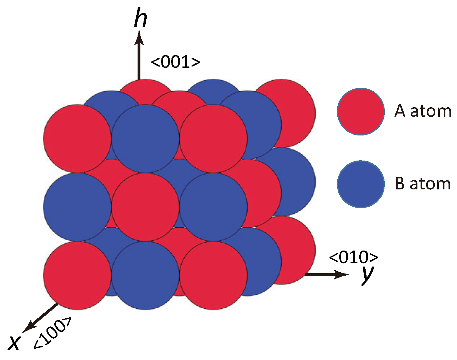
2.1. Surface Hamiltonian

An AB compound is made of A and B atoms in the ambient phase as follows:

$$A+B⟷AB.$$

(5)

Let us define ${\mu }_{\mathrm{A},\mathrm{ambient}}$ (${\mu }_{\mathrm{B},\mathrm{ambient}}$) to be the bulk chemical potential of A atoms (B atoms) in the ambient phase. Let us consider an NaCl-type crystal structure (Figure 1) of an AB compound, where ${\mu }_{\mathrm{A},\mathrm{crys}}$ (${\mu }_{\mathrm{B},\mathrm{crys}}$) is the bulk chemical potential of A atoms (B atoms) in the AB compound (Appendix A). The {111} and {001} surfaces are the polar and non-polar surfaces, respectively. Here, the chemical potential of the AB compound ${\mu }_{\mathrm{AB},\mathrm{crys}}$ is defined by [38,40,47]

$${\mu }_{\mathrm{AB},\mathrm{crys}}={\mu }_{\mathrm{A},\mathrm{crys}}+{\mu }_{\mathrm{B},\mathrm{crys}}.$$

(6)

To study the surface roughness of a vicinal surface, the st-RSOS model [42], which is a staggered 19-vertex model [43,44], is adopted for the microscopic model in the Monte Carlo method. Here, “restricted” means that the height difference between nearest-neighbor sites is restricted to $\{0,\pm 1\}$. The surface Hamiltonian is given by the following equation:

$$\begin{array}{ccc}\hfill \mathcal{H}& =& {\displaystyle \sum _{\{m,n\}}}\{ϵ[|h(m+1,n,{\sigma }^{\prime })-h(m,n,\sigma )|+|h(m,n+1,{\sigma }^{″})-h(m,n,\sigma )|]\hfill \\ & -& \Delta \mu h(m,n,\sigma )-\frac{\Delta {\mu }_A}{2}{\delta }_{(h(m,n)+m+n),even}-\frac{\Delta {\mu }_B}{2}{\delta }_{(h(m,n)+m+n),odd}\}\hfill \\ & & +\mathcal{N}(E_{A,\mathrm{surf}}+E_{B,\mathrm{surf}}),\hfill \end{array}$$

(7)

where $h(m,n,\sigma )$ is the height of the surface at a site $(n,m)$ with atomic species $\sigma =$A or B, $ϵ$ is half the lateral effective bond energy between nearest-neighbor atoms (microscopic ledge energy), $\mathcal{N}$ is the total number of unit cells on the (001) surface, and $E_{A,\mathrm{surf}}$ ($E_{B,\mathrm{surf}}$) is the surface energy at a site for A atoms (B atoms) per half-unit cell. The RSOS condition is implicitly required. Here, $\Delta {\mu }_A$, $\Delta {\mu }_B$, and $\Delta \mu$ are introduced as follows:

$$\begin{array}{ccc}\hfill \Delta {\mu }_A& =& {\mu }_{\mathrm{A},\mathrm{ambient}}-{\mu }_{\mathrm{A},\mathrm{crys}},\Delta {\mu }_B={\mu }_{\mathrm{B},\mathrm{ambient}}-{\mu }_{\mathrm{B},\mathrm{crys}}\hfill \\ \hfill \Delta \mu & =& (\Delta {\mu }_A+\Delta {\mu }_B)/2.\hfill \end{array}$$

(8)

Here, the number of atoms in the crystal or ambient phase is not fixed. The atoms in the ambient phase are captured by the vicinal surface; the atoms on the outermost layer of the crystal can escape to the ambient phase. Hence, in the statistical system under consideration, a grand canonical ensemble is adopted. The third and fourth (fifth) terms on the right-hand side of Equation (7) indicate the energy gain that an A- (B-) atom transfers from the ambient phase to the crystal. When $h(m,n)+m+n$ is even (odd), the transferred atom is A (B). The partition function in Equation (7) $\mathcal{Z}(T,\Delta {\mu }_A,\Delta {\mu }_B)$ is the grand partition function, and the thermodynamic potential $\mathsf{\Phi }(T,\Delta {\mu }_A,\Delta {\mu }_B)=(1/\mathcal{N})(-k_{\mathrm{B}}T)ln\mathcal{Z}(T,\Delta {\mu }_A,\Delta {\mu }_B)$ is the grand potential.

Because an AB compound is studied, the equilibrium condition at two-phase coexistence is given by [38,39,40,63,64]

$${\mu }_{A,\mathrm{crys}}+{\mu }_{B,\mathrm{crys}}={\mu }_{A,\mathrm{ambient}}+{\mu }_{B,\mathrm{ambient}}.$$

(9)

From Equations (8) and (9), we obtain the following Gibbs–Duhem equation:

$$\Delta \mu =0,\Delta {\mu }_B=-\Delta {\mu }_A.$$

(10)

Here, the steps covered by A atoms (B atoms) are referred to as A steps (B steps). For $\Delta {\mu }_A>0$, an A step has lower energy than a B step because of the fourth and fifth terms on the right-hand side of Equation (7). Because the (111) surface is a close-packed arrangement of steps, the ${(111)}_A$ surface has lower energy than that of the ${(111)}_B$ surface. This has been experimentally confirmed by Nishizawa and Pons [41]. Based on the energy Hamiltonian in Equation (7), the surface roughness for a vicinal surface tilted towards the $\langle 111\rangle$ direction is studied.

When the ambient phase is a gas, $\Delta {\mu }_A$ and $\Delta {\mu }_B$ are expressed as follows assuming an ideal gas (Appendix A):

$$\Delta {\mu }_A=k_{\mathrm{B}}Tln(P_A/P_{A0}),\Delta {\mu }_B=k_{\mathrm{B}}Tln(P_B/P_{B0}),$$

(11)

where $P_A$ ($P_B$) is the partial pressure of A atoms (B atoms) in the bulk gas phase. Instead of using ${\mu }_{A,\mathrm{crys}}$ or ${\mu }_{B,\mathrm{crys}}$, ${\mu }_{A,\mathrm{gas}}$ and ${\mu }_{B,\mathrm{gas}}$ are used so that

$${\mu }_{A,\mathrm{crys}}={\mu }_{A,\mathrm{ambient}},{\mu }_{B,\mathrm{crys}}={\mu }_{B,\mathrm{ambient}}.$$

(12)

$P_{A0}$ ($P_{B0}$) is the partial pressure determined by the condition in Equation (12) (Appendix A). Hence, we obtain Equation (11).

It should be noted that the dominant contribution to $\Delta {\mu }_A$ or $\Delta {\mu }_B$ is the mixed entropy in the ambient phase. Irrespective of the atomic species, the thermodynamic effect of the concentration deviation in the ambient phase can be determined from the change in $\Delta {\mu }_A$ or $\Delta {\mu }_B$. As an example, when the ambient phase is a solution, $\Delta {\mu }_A$ and $\Delta {\mu }_B$ are expressed as follows assuming an ideal solution:

$$\Delta {\mu }_A=k_{\mathrm{B}}Tln(c_A/c_{A0}),\Delta {\mu }_B=k_{\mathrm{B}}Tln(c_B/c_{B0}),$$

(13)

where $c_A$ ($c_B$) is the concentration of A atoms (B atoms) and $c_{A0}$ ($c_{B0}$) is their concentration under the condition in Equation (12).

The bulk chemical potentials and the surface energies for the flat (001) surface should be calculated using the first-principles DFT method [45,46,47,48,49,50]. However, the surface model expressed by the Hamiltonian in Equation (7) is slightly more coarse-grained compared to the surface structure considered in the first-principles DFT calculations. In the model of Equation (7), $ϵ$ or $E_{A,\mathrm{surf}}$ ($E_{B,\mathrm{surf}}$) is considered to correspond to the surface free energy per half-unit cell in the DFT calculations. Hence, ${\mu }_{A,\mathrm{crys}}$ (${\mu }_{B,\mathrm{crys}}$) $\approx zϵ$ with $z=6$, where z is the number of nearest-neighbor sites in the bulk crystal, $E_{A,\mathrm{surf}}\approx E_{B,\mathrm{surf}}\approx ϵ$. According to a recent study by Kempisty et al. [50], the surface free energy decreases as the temperature increases due to the entropy caused by distortions or vibrations. Hence, $ϵ$, $P_{A0}$, $P_{B0}$, $c_{A0}$, and $c_{B0}$ depend on temperature.

2.2. Monte Carlo Method

To study the effects of a stoichiometric deviation in the ambient phase, the Monte Carlo method for non-conserved systems is used. Here, “non-conserved” indicates that the number of crystals is not conserved. Atoms on the crystal surface can escape to the ambient phase or be captured from the ambient phase. Hence, surface and volume diffusion are not taken into consideration.

The vicinal surface around the (001) surface tilted towards the (111) direction is considered using the Monte Carlo method with the Metropolis algorithm. The external parameters are temperature T, $\Delta {\mu }_A$, number of steps $N_{\mathrm{step}}$, and the linear size of the system L.

Initially, $N_{\mathrm{step}}$ steps run in the mean direction $\tilde{y}=\langle \overline{1}10\rangle$, for which the periodic boundary condition is required. The $\tilde{x}$ direction is assigned to the $\langle 110\rangle$ direction. The configurations on the lower side (right side of the top-down view of the surface, e.g., Figure 2a) are connected to the upper side (left side of the top-down view of the surface) by adding $N_{\mathrm{step}}a$. We consider two types of initial surface configuration: a surface with a macrostep where all steps assemble, and a surface with a train of steps.

The lattice sites on the surface at which an event occurs are selected randomly. “Capture” or “escape” for the lattice site is selected randomly with a probability of 1/2. The energy change between the states before and after an event is calculated using Equation (7). If the energy change is negative, the surface configuration is updated with a probability of 1. If the energy change is positive, the surface configuration is updated with a probability of $exp[-(E_{\mathrm{after}}-E_{\mathrm{before}})/k_{\mathrm{B}}T]$. Here, $E_{\mathrm{after}}$ ($E_{\mathrm{before}}$) is the surface energy calculated using Equation (7) after (before) the surface configuration update.

The capture or escape of atoms on the (001) terrace surface occurs at equilibrium. Because surface diffusion of atoms is not taken into consideration, the advance and recession of an elementary step are, respectively, caused by the capture and escape of atoms at kinks on step edges. Snapshots of the top-down and side views of the simulated surface at $4\times {10}^8$ Monte Carlo steps per site (MCS/site) are shown in Figure 2. It should be noted that the elementary steps have few kinks on step edges for $\Delta {\mu }_A/ϵ=2$. We will return to this point in the following sections.

The mean surface profile normal to the mean running direction of elementary steps is calculated as follows:

$$\begin{array}{ccc}\hfill \langle h\rangle (\tilde{x},t)& =& \frac{\sqrt{2}a}{L}{\displaystyle \sum _{\tilde{y}=1}^{L/(\sqrt{2}a)}}h(\tilde{x},\tilde{y},t),\hfill \end{array}$$

(14)

where the $\tilde{y}$ and $\tilde{x}$ directions are, respectively, parallel and normal to the mean running direction of elementary steps. In the present study, $\tilde{y}$ and $\tilde{x}$ are, respectively, in the $\langle \overline{1}10\rangle$ and $\langle 110\rangle$ directions. In Figure 3a, an example of a mean surface profile is shown with a size of $320\sqrt{2}a$ ($a=1$) at $4\times {10}^8$ MCS/site. The homogeneous slope of the surface can be seen.

The mean surface height $\overline{h}$ is calculated as follows:

$$\overline{h}(t)=\frac{\sqrt{2}a}{L}\sum _{\tilde{x}=1}^{L/(\sqrt{2}a)}\langle h\rangle (\tilde{x},t).$$

(15)

In Figure 4, time evolutions of the mean surface height are shown for several $\Delta {\mu }_A$ values. The fluctuations of the location of the surface are relatively large for $\Delta {\mu }_A/ϵ=0$ and 4. As shown, there are long-time fluctuations around a mean value. We will return to this point in Section 3.3. However, there is no systematic increase or decrease in surface height. Hence, the systems are at equilibrium as expected.

The square of the surface width $W^2(\tilde{x},L)$ is defined by the variance of the surface height, which is calculated as

$$\begin{array}{ccc}\hfill g{W}^2(\tilde{x},L)& =& \frac{\sqrt{2}a}{({\tau }_{\max }-{\tau }_0)L}\times {\displaystyle \sum _{t={\tau }_0}^{{\tau }_{\max }}\sum _{\tilde{y}=1}^{L/(\sqrt{2}a)}}\left[{(h(\tilde{x},\tilde{y},t)-\langle h\rangle (\tilde{x},t))}^2\right],\hfill \\ \hfill g& =& (1+p_x^2+p_y^2)=1/{cos}^2\theta ,\hfill \\ \hfill p_x& =& \langle \frac{\partial h(x,y)}{\partial x}\rangle ,p_y=\langle \frac{\partial h(x,y)}{\partial y}\rangle ,\hfill \end{array}$$

(16)

where g is a metric for a tilted surface [35], $\theta$ is the angle of the tilt towards the $\langle 111\rangle$ direction, ${\tau }_0=2\times {10}^8$ and ${\tau }_{\max }=4\times {10}^8$ MCS/site are the averaged times, and $p_x$ and $p_y$ are the surface gradients. In the present Monte Carlo simulations, $\overline{p_x}=\overline{p_y}=3/8=0.375$ and $\overline{p}=\sqrt{p_x^2+p_y^2}=3\sqrt{2}/8=0.530$.

An example of the calculated $g{W}^2(\tilde{x},L)$ is shown in Figure 3b. Although the surface is tilted, the square of the surface width is constant with respect to $\tilde{x}$. We determine $g{W}^2(L)$ as the averaged $g{W}^2(\tilde{x},L)$, fitted using the least squares method.

3. Decrease in Roughness Due to Locally Merged Steps

3.1. Mean Height of Local Merged Steps

To study whether a macrostep is self-organized, we calculate the mean height of merged steps $\langle n\rangle$ as follows:

$$\langle n\rangle =\sum _{\tilde{y}}\sum _{\tilde{x}}|n_{\tilde{x}}(\tilde{y})|/\left[\sum _{\tilde{y}}{n}_{\mathrm{step}}(\tilde{y})\right],$$

(17)

where $n_{\mathrm{step}}(\tilde{y})$ is the number of macrosteps at $\tilde{y}$ along the $\tilde{x}$ direction. $\langle n\rangle$ is averaged over from ${\tau }_0$ to ${\tau }_{\max }$. The obtained $\langle n\rangle$ is shown in Figure 5a. The values of $\langle n\rangle$ with respective $\Delta {\mu }_A$ agree with the values of $\langle n\rangle$ with $-\Delta {\mu }_A$ within the errors. Near $\Delta {\mu }_A\approx 0$, $\langle n\rangle$ is about 1.1, which means that the elementary steps are well separated. This can be seen in Figure 2a.

Around $\Delta {\mu }_A/ϵ\approx 2$, however, there is a broad peak that diminishes when the size of the system increases. Double steps covered by A atoms appear in Figure 2b. There are few kinks on the edges of the elementary steps. Because the peak disappears in large systems, it is considered to be caused by a finite size effect. The zig-zag structure of steps causes entropic repulsion between steps. The small number of kinks in the small system weakens this repulsive interaction between steps. In addition, once neighboring steps in the small system arrive at a close-packed location, kink formation becomes difficult due to the RSOS geometrical restriction.

For $1\le \Delta {\mu }_A/ϵ\le 3$, $\langle n\rangle$ is about 1.25 for a large system. The fraction of double steps c is estimated using the following equation:

$$\langle n\rangle =2C_2+1\times (1-C_2).$$

(18)

We have $C_2=0.25$ for $\langle n\rangle =1.25$ (Figure 5b). For a small system, $\langle n\rangle$ has a maximum value of 1.7 near $\Delta {\mu }_A/ϵ\approx 2$. We have $C_2=0.7$. This means that 70% of elementary steps form double steps for a small system.

For $\Delta {\mu }_A/ϵ\ge 4$, $\langle n\rangle$ increases to 2.5 as $\Delta {\mu }_A$ increases. A snapshot of the surface for $\Delta {\mu }_A/ϵ=5.0$ is shown in Figure 2d. Almost the whole vicinal surface is covered by A atoms. Assuming that the vicinal surface consists of double steps and quadruple steps, we have

$$\langle n\rangle =4C_4+2\times (1-C_4),$$

(19)

where $C_4$ is the fraction of quadruple steps (Figure 5b).

3.2. No Step Faceting

As described in the previous subsection, double and quadruple merged steps are observed locally. However, macrosteps that run from edge to edge are not observed. For a macrostep to form on a vicinal surface at equilibrium, a first-order transition on the surface free energy with respect to the surface orientation is required [3,65]. This can be seen in the Wulff figure, which is the polar graph of surface tension [66,67,68].

At finite temperature for the original RSOS model, the surface tension ${\gamma }_{\mathrm{surf}}$ decreases owing to surface entropy per area $s_{\mathrm{surf}}$ as the temperature increases, because ${\gamma }_{\mathrm{surf}}=E_{\mathrm{surf}}-T{s}_{\mathrm{surf}}$ [5]. The (001) surface is thermally roughened at the roughening transition temperature ${T_{\mathrm{R}}}^{(001)}$ [15,20]. The order of the roughening transition is the Kosterlitz–Thouless–type continuous transition [20]. The ${T_{\mathrm{R}}}^{(001)}$ of the original RSOS model was calculated by den Nijs to be approximately $k_{\mathrm{B}}{T_{\mathrm{R}}}^{(001)}/ϵ=1.580$ [69]. The step tension on the (001) surface decreases to zero at ${T_{\mathrm{R}}}^{(001)}$ as the temperature increases [20]. The (001) facets on the ECS shrink with increasing temperature, vanishing at ${T_{\mathrm{R}}}^{(001)}$. This shape transition is called the faceting transition [22,23,26]. The temperature dependence of the (001) facet-shapes on the ECS has been studied by several researchers [22,70,71].

For the st-RSOS model, the (001) surface and the ECS also cause roughening and faceting transitions at ${T_{\mathrm{R}}}^{(001)}$, respectively. In addition, ${T_{\mathrm{R}}}^{(001)}$ depends on the component deviation in the ambient phase $\Delta {\mu }_A$. We first study the stoichiometric change in the Wulff figures at $T=0$ K. Cross-sections of the Wulff figures obtained at $T=0$ K for the st-RSOS model are shown in Figure 6. The figures show how the change in relative chemical potential in the ambient phase affects the surface tension for $\Delta {\mu }_A\ge 0$. The ECS is also shown. At $\Delta \mu =0$, the surface tension of the A surface equals that of the B surface and the ECS for the (111)A surface agrees with that for the (111)B surface. For $0<\Delta {\mu }_A/ϵ<4$, the surface tension of the A surface (dark blue lines) is lower than that of the B surface (light blue lines). Because the surface tension of the A surface is smaller than that of the B surface, the ECS with the (111)A surface (red full lines) is realized. For $\Delta {\mu }_A/ϵ\ge 4$, the (001) surface does not appear because it is roughened stoichiometrically. At $\Delta {\mu }_A/ϵ=6$, the surface energy of the (111) surface becomes zero. For $\Delta {\mu }_A/ϵ>6$, the surface energy of the (111) surface is negative, and thus, the system becomes unphysical.

Because surfaces and steps are low-dimensional objects, thermal fluctuations are often sufficient to destroy the ordered phase at finite temperature in a system based on short-range forces [72]. The calculation of the surface free energy using a mean field or quasi-chemical approximation for low-dimensional objects often leads to incorrect results. Hence, calculations more precise than those obtained from mean field approximation are required. However, such calculations are quite difficult for the st-RSOS model.

At temperatures sufficiently lower than ${T_{\mathrm{R}}}^{(001)}$, the (001) surface is well approximated by a 2D lattice gas model [73,74]. The lattice gas model causes a second-order 2D Ising-type phase transition at $T_c$. Although ${T_{\mathrm{R}}}^{(001)}$ is known to be higher than $T_c$, we can calculate the $\Delta {\mu }_A$ dependence of $T_c$ using the imaginary-path-weight random walk (IPW) method [75,76,77,78,79] based on a 2D lattice gas model (Appendix B). The $\Delta {\mu }_A$ dependence of $T_c$ is shown by the broken line in Fig. 13(a) in Ref. [40] ($H/J=\Delta {\mu }_A/ϵ$) as a critical curve under the assumption that $ϵ$ is constant. The temperature on the critical curve at $\Delta {\mu }_A=0$ equals ${k_{\mathrm{B}}T}_c/ϵ=1/ln(1+\sqrt{2})\approx 1.13459$ ($={k_{\mathrm{B}}T}_c/(2J)$). $\Delta {\mu }_{Ac}/ϵ$ on the critical curve at $T=0$ and $k_{\mathrm{B}}T/ϵ=0.2$ equals 4 and 3.7227, respectively [40].

The $\Delta {\mu }_A$ dependence of facet shapes at $k_{\mathrm{B}}T/ϵ=0.2$ is shown in Figure 7 [40,74]. As seen from the figures, the anisotropy of the surface tension and the facet shape depends on $\Delta {\mu }_A$. The area of the facet shape shrinks as $\Delta {\mu }_A$ increases, becoming zero at a temperature $k_{\mathrm{B}}T/ϵ=0.2$ with $\Delta {\mu }_{Ac}/ϵ=3.7227$. The morphology of the surface obeys not only the symmetry of the energy Hamiltonian but also the geometrical symmetry of the crystal structure. This geometrical situation causes non-monotonic changes of $g{W}^2(L)$, $\langle n\rangle$, and step quantities with respect to $\Delta {\mu }_A$.

The formation of macrosteps at equilibrium requires a first-order shape transition [23], which leads to discontinuous surface tension [3,8]. However, the Wulff figures do not show such a discontinuity in the present case. To obtain discontinuous surface tension at low temperature, the point-contact-type step–step attraction that originates from the quantum mechanical interactions between steps [10] is required. The present Monte Carlo study does not produce macrosteps. Therefore, a stoichiometric deviation in the ambient phase does not cause global macrosteps.

3.3. $\Delta {\mu }_A$ Dependence of Surface Roughness

The obtained $\Delta {\mu }_A$ dependence of $g{W}^2(L)$ for the st-RSOS model is shown in Figure 8. The values obtained for different initial configurations agree well with each other. In contrast to $\langle n\rangle$, $g{W}^2(L)$ has a minimum at around $\Delta {\mu }_A/ϵ=2$. Regarding the roughness of the vicinal surface, this behavior of $g{W}^2(L)$ is consistent with long-term height fluctuation up to $\Delta {\mu }_A/ϵ\sim 4$ (Figure 4). Because the number of atoms in the surface area is an internal parameter, it fluctuates. Although the (001) surface is smooth, the capture and escape of atoms (units) on the (001) surface occur at equilibrium. Wandering of the parallel train of steps [33,35] on the vicinal surface is caused by the atomic capture and escape processes at kinks on step edges. The change in the (001) surface roughness is thus not the dominant factor in the change in $g{W}^2(L)$. More importantly, the change in kink density on step edges and the change in the fraction of double and quadruple steps are mainly responsible for the $g{W}^2(L)$ change for $|\Delta {\mu }_A/ϵ|\stackrel{<}{\sim }4$.

However, for $\Delta {\mu }_A/ϵ>4$, both the vicinal surface and the (001) surface are rough. The vicinal surface is covered with A atoms and the elementary step height is $2a$. The edge of a double A step has overhanging structures (Figure 2d), which are typical for a thermally roughened (001) surface. The intrinsic width of a step [80,81] is infinitely large for a thermally roughened surface.

However, the mean height fluctuation shown in Figure 4d is small. This is because the concentration of B atoms in the ambient phase is insufficient to grow or recede the surface.

4. Surface Roughness

4.1. Effect of Component Deviation on Roughness Exponent

The size dependence of $g{W}^2(L)$ for $|\Delta {\mu }_A/ϵ|<4$ is shown in Figure 9. From Figure 9b, it can be clearly seen that $g{W}^2(L)$ increases logarithmically as L increases for large L. The logarithmic divergence of the surface width for high $|\Delta \mu |$, such that $|\Delta \mu /ϵ|=\{4,5\}$, is shown in Figure 10. Therefore, $\alpha =0$ for all $\Delta {\mu }_A$. This behavior is consistent with previously reported results for thermally roughened surfaces (interfaces) [26,37]. These results indicate that a stoichiometric deviation in the ambient phase does not affect the roughness exponent for a large system.

4.2. Mean Free Length

According to the linear theory of molecular beam epitaxy (MBE), the time evolution of the surface can be expressed by the following equation [34]:

$$\frac{\partial h}{\partial t}=\nu {\nabla }^{2}h-K{\nabla }^{4}h+\eta .$$

(20)

where h is the surface height, $\nu$ is the surface tension, K is a constant related to surface diffusion, and $\eta$ is a random force. The competition between the terms ${\nabla }^{2}h$ and ${\nabla }^{4}h$ generates a characteristic length $L_{1,\mathrm{MBE}}$, which is expressed by [34]

$$L_{1,\mathrm{MBE}}=\sqrt{K/\nu }.$$

(21)

For $L<L_{1,\mathrm{MBE}}$, ${\nabla }^{4}h$ is dominant. Hence, the roughness exponent $\alpha$ is $(4-d)/2$, where d is the spatial dimension. For $L>L_{1,\mathrm{MBE}}$, ${\nabla }^{2}h$ is dominant, and thus $\alpha$ is $(2-d)/2$.

Because Equation (20) is derived from the symmetry principle [34], the linear theory with $K=0$ is applicable to a crystal and solution system, such as SiC in Si fluid. In the present study, because $d=2$ and $K=0$, we have $L_{1,\mathrm{MBE}}=0$ from Equation (21). Hence, $g{W}^2(L)$ is expected to behave logarithmically for all L. However, as shown in Figure 9, there exists another characteristic length $L_1$.

As shown in Figure 9b, the calculated $g{W}^2(L)$ deviates from the logarithmic behavior on the short length scale. First, the Monte Carlo data of $L\ge 160\sqrt{2}$ in Figure 9b are fitted to the following equation:

$$\begin{array}{ccc}\hfill g{W}^2{(L)}_{\mathrm{fit}}/a^2& =& A[ln(L)-ln(L_{\mathrm{MFL}})]+y_0,\hfill \\ \hfill a& =& 1,y_0=0.147,\hfill \end{array}$$

(22)

where A is the amplitude and $L_{\mathrm{MFL}}$ is the mean free length defined in Equation (22). The obtained A and $L_{\mathrm{MFL}}$ are listed in

Table 1. Characteristic lengths, step tension, and step stiffness.

	Amplitude			Step Tension	Step Stiffness
ΔμA/ϵ	A	LMFL	${\mathit{L}}_{\mathbf{MFL}}/{\mathit{L}}_{\mathbf{MFL}}{|}_{\Delta {\mathit{\mu }}_{\mathit{A}}=\mathit{0}}$	$\mathit{\gamma }/\mathit{J}$	$\tilde{\mathit{\gamma }}/\mathit{J}$	${\mathit{\gamma }}_{\mathit{m}}{/\mathit{\gamma }|}_{\Delta {\mathit{\mu }}_{\mathit{A}}=0}$	${\tilde{\mathit{\gamma }}}_{\mathit{m}}/\tilde{\mathit{\gamma }}{|}_{\Delta {\mathit{\mu }}_{\mathit{A}}=0}$
	Equation (22)	Equation (22)		Ref. [40]	Ref. [40]	ϕ = 45°	ϕ = 45°
0.0	0.0739	6.1	1	2.44	0.565	1	1
1.0	0.0928	31	5.0	2.08	2.00	1.07	4.42
2.0	0.0907	156	26	1.41	10.5	0.722	23.2
3.0	0.1015	24	3.9	0.662	1.45	0.340	3.21
4.0	0.203	2.7	0.45	0	0	0	0
5.0	0.280	2.1	0.35	0	0	0	0

.

$L_{\mathrm{MFL}}$ has a maximum value at around $\Delta {\mu }_A/ϵ=2.0$. The ratio between $L_{\mathrm{MFL}}$ and $L_{\mathrm{MFL}}{|}_{\Delta {\mu }_A=0}$ is shown in the fourth column in Table 1. As shown in Figure 2b, there are few kinks on a given step. To see what happens on the surface at $\Delta {\mu }_A/ϵ=2.0$, we consider a 2D lattice gas model for the two-component system.

4.3. Analysis Based on Two-Dimensional Lattice Gas Model

Step tension $\gamma$, which is the step free energy per unit length, and step stiffness $\tilde{\gamma }=\gamma +{\partial }^2\gamma /\partial {\varphi }^2$, where $\varphi$ is the tilt angle between the mean step running direction and the y direction ([010] direction), can be calculated based on the surface configuration energy in Equation (A11). Because a step is a 1D object, the entropy is significant in low dimensions [72]. Hence, entropy calculation that is more precise than mean field or quasi-chemical approximation is required.

The step tension and step stiffness are calculated precisely using the IPW method [40,75,76,77,78,79] (Figure 7 and Figure 11). The calculated step tension and step stiffness are shown in Table 1 in the fifth and sixth columns, respectively.

Due to the mixing of single and double steps for $1\le \Delta {\mu }_A/ϵ<4$, ${\gamma }_m$ and ${\tilde{\gamma }}_m$ are considered to be

$$\begin{array}{ccc}\hfill {\gamma }_m& =& [(1-C_2)+2C_2]\gamma ({45}^{\circ }),\hfill \\ \hfill {\tilde{\gamma }}_m& =& [(1-C_2)+2C_2]\tilde{\gamma }({45}^{\circ })\mathrm{with}{C}_2=0.25.\hfill \end{array}$$

(23)

The ratios ${\gamma }_m{/\gamma |}_{\Delta {\mu }_A=0}$ and ${\tilde{\gamma }}_m/\tilde{\gamma }{|}_{\Delta {\mu }_A=0}$ are shown in the seventh and eighth columns of Table 1, respectively.

According to Equation (20), surface tension may explain the $\Delta {\mu }_A$ dependence of $L_{\mathrm{MFL}}$. The surface tension ${\gamma }_{\mathrm{surf}}$, which is the surface free energy per normal area, is expressed by ${\gamma }_{\mathrm{surf}}\approx {\gamma }_m\rho$, where $\rho$ is the step density, for the lowest order with respect to $\rho$. However, the $\Delta {\mu }_A$ dependence of the surface tension or the step tension (seventh column in Table 1) is different from that of $L_{\mathrm{MFL}}/L_{\mathrm{MFL}}{|}_{\Delta {\mu }_A=0}$. That is, Equation (20) cannot explain the results of $L_{\mathrm{MFL}}/L_{\mathrm{MFL}}{|}_{\Delta {\mu }_A=0}$.

The $\Delta {\mu }_A$ dependence of the ratio ${\tilde{\gamma }}_m/\tilde{\gamma }{|}_{\Delta {\mu }_A=0}$ (eighth column in Table 1) is similar to that of $L_{\mathrm{MFL}}/L_{\mathrm{MFL}}{|}_{\Delta {\mu }_A=0}$. In the following subsection, the relationship between step stiffness and the mean free length is examined.

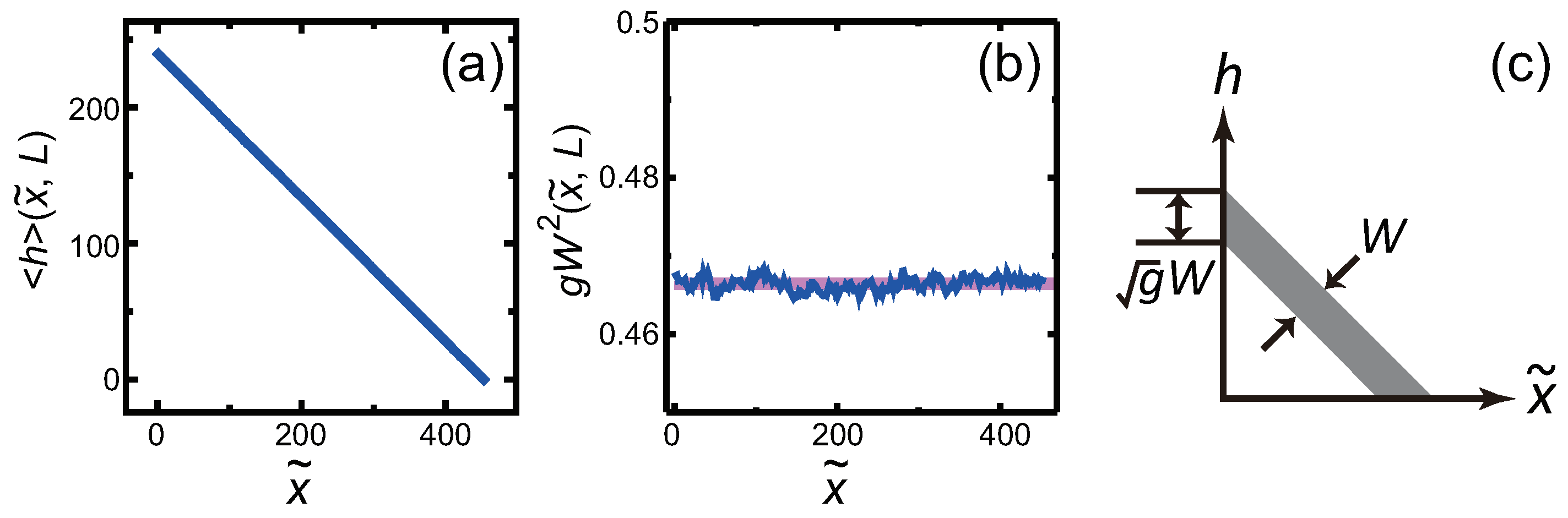
4.4. Relationship between Surface Width and Step Width

For single steps, the step width $w_{s,\mathrm{single}}(L)$ is estimated using a 1D free random walk such that $w_{s,\mathrm{single}}^2(L)=L\sigma$, where L is the mean running distance of a step along the step and $\sigma$ is the scaled step width. In the 1D free random walk, L corresponds to time and $\sigma$ corresponds to the diffusion constant. $\sigma$ is related to the stiffness of a single step [82] as follows:

$$w_{s,\mathrm{single}}^2(\tilde{y})/\tilde{y}={\sigma }^2=k_{\mathrm{B}}T/\tilde{\gamma }=\frac{k_{\mathrm{B}}T}{\lambda }\kappa ,$$

(24)

where $\lambda$ is related to the volume of a 2D island with an equilibrium shape and $\kappa$ is the curvature of the edge of the island. For a vicinal surface, steps collide with neighboring steps. This step collision changes the squared fluctuation width of a single step from linear L to $logL$ [36,37].

Recall the relationship between surface height–height correlation $G(\tilde{x},\tilde{y})$ and the step width ${\Delta }_{s,\mathrm{vicinal}}^2(\tilde{y}))$ [36,37] (Figure 12a) on a vicinal surface:

$${\Delta }_{s,\mathrm{vicinal}}^2(\tilde{y})=\frac{1}{{\rho }^2}G(0,\tilde{y}),$$

(25)

where $G(0,\tilde{y})$ is

$$\begin{array}{ccc}\hfill G(0,\tilde{y})& =& \langle {[h(\tilde{x},\tilde{y},t)-h(\tilde{x},0,t)]}^2\rangle \hfill \\ & \to & \tilde{A}ln(\tilde{y}),(\tilde{y}\to \infty ),\hfill \end{array}$$

(26)

where $\tilde{A}$ is the amplitude. $G(0,\tilde{y})=2g{W}^2$ in a large L limit.

Then, let us introduce $L_{\mathrm{MFL},g}$ as a length, with which an individual step makes contact with neighboring steps (Figure 12b):

$$L_{\mathrm{MFL},g}{\sigma }^2={\ell }^2=1/({\rho }^2),$$

(27)

where ℓ is the mean step distance. Substituting Equation (24) into Equation (27), we have

$$L_{\mathrm{MFL},g}=\frac{\tilde{\gamma }}{{\rho }^2{k}_{\mathrm{B}}T}.$$

(28)

For $\tilde{y}<L_{\mathrm{MFL},g}$, we have the following equations:

$$\begin{array}{ccc}\hfill G(0,\tilde{y})& =& {\rho }^2{\Delta }_{s,\mathrm{vicinal}}^2(\tilde{y})\hfill \\ & \approx & {\rho }^2{w}_{s,\mathrm{single}}^2(\tilde{y})={\rho }^2{\sigma }^2\tilde{y}\hfill \\ & =& \tilde{y}/L_{\mathrm{MFL},\mathrm{g}}.\hfill \end{array}$$

(29)

For $\tilde{y}>L_{\mathrm{MFL},g}$, $G(0,\tilde{y})$ increases logarithmically with respect to $\tilde{y}$, as shown in Equation (26). Assuming

$$L_{\mathrm{MFL}}=s{L}_{\mathrm{MFL},g},s\approx 1.7,$$

(30)

we have

$$g{W}^2=L/(2L_{\mathrm{MFL}}),(\tilde{y}\sim L).$$

(31)

Here, s is a parameter related to the mixture of merged steps.

Equations (28), (30) and (31) well explain the $\Delta {\mu }_A$ dependence of $L_{\mathrm{MFL}}$ and $g{W}^2(L)$ for small L.

4.5. Small Systems

When ℓ is assumed to be a (=1), $L_{\mathrm{MFL},g}$ expresses the mean distance between kinks on the step edge. We denote this quantity as $L_{\mathrm{kink}}$. From Equations (24) and (27), we have

$$L_{\mathrm{kink}}=a^2\tilde{\gamma }/k_{\mathrm{B}}T,(a=1).$$

(32)

Around $\Delta {\mu }_A=2$, $L_{\mathrm{kink}}$ estimated from the value of the step stiffness is $26a$. This result is consistent with Figure 2b. When the system size is sufficiently small, there are no kinks on the step edge. In such a situation, the surface is similar to a smooth surface. Hence, $g{W}^2(L)$ is almost constant, rather than proportional to L, as shown by Equation (29). The deviation from the logarithmic behavior around $\Delta {\mu }_A/ϵ=2$ (Figure 9) confirms this.

$L_{\mathrm{kink}}$ can also be observed using the method proposed by Swartzentruber et al. [83,84,85]. For $L<L_{\mathrm{kink}}$, phenomena similar to 1D nucleation [86] may occur at an elementary step edge. Due to the entropy effect in low dimensions [72], 1D nucleation does not typically occur [87]. However, when the system size is sufficiently small ($L<L_{\mathrm{kink}}$), 1D-nucleation-like phenomena may occur in a practical case of crystal growth.

When the temperature is higher than that in the present study, step stiffness decreases, becoming more isotropic. $L_{\mathrm{MFL}}$ and $L_{\mathrm{kink}}$ decrease according to Equations (28) and (32), respectively. When the temperature is lower, the anisotropy of step stiffness becomes stronger. Hence, $L_{\mathrm{MFL}}$ around $\Delta \mu /ϵ\sim 2$ becomes substantially larger.

This is consistent with the models used in the first-principles quantum mechanical calculation of the surface. In the quantum mechanical calculation, the model is assumed to contain several unit cells in a flat area. The surface is assumed to be smooth. However, on a mesoscopic scale, the vicinal surface is rough. Our results resolve this conflict and connect the quantities calculated using quantum mechanics to the hydrodynamic model.

5. Conclusions

For a stoichiometric two-component crystal, this study investigated the effects of the component deviation in the ambient phase on the assembly and disassembly of elementary steps on a vicinal surface using the Monte Carlo method based on the st-RSOS model.

The global behavior of the vicinal surface can be summarized as follows:

• A component deviation in the ambient phase $\Delta {\mu }_A$ does not cause macrostep self-organization.
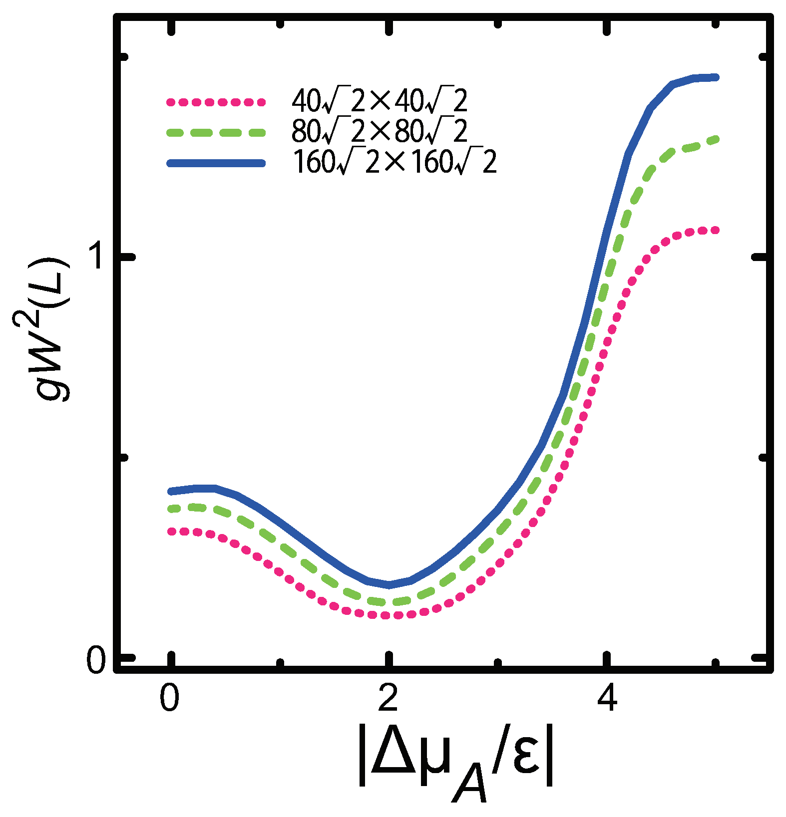
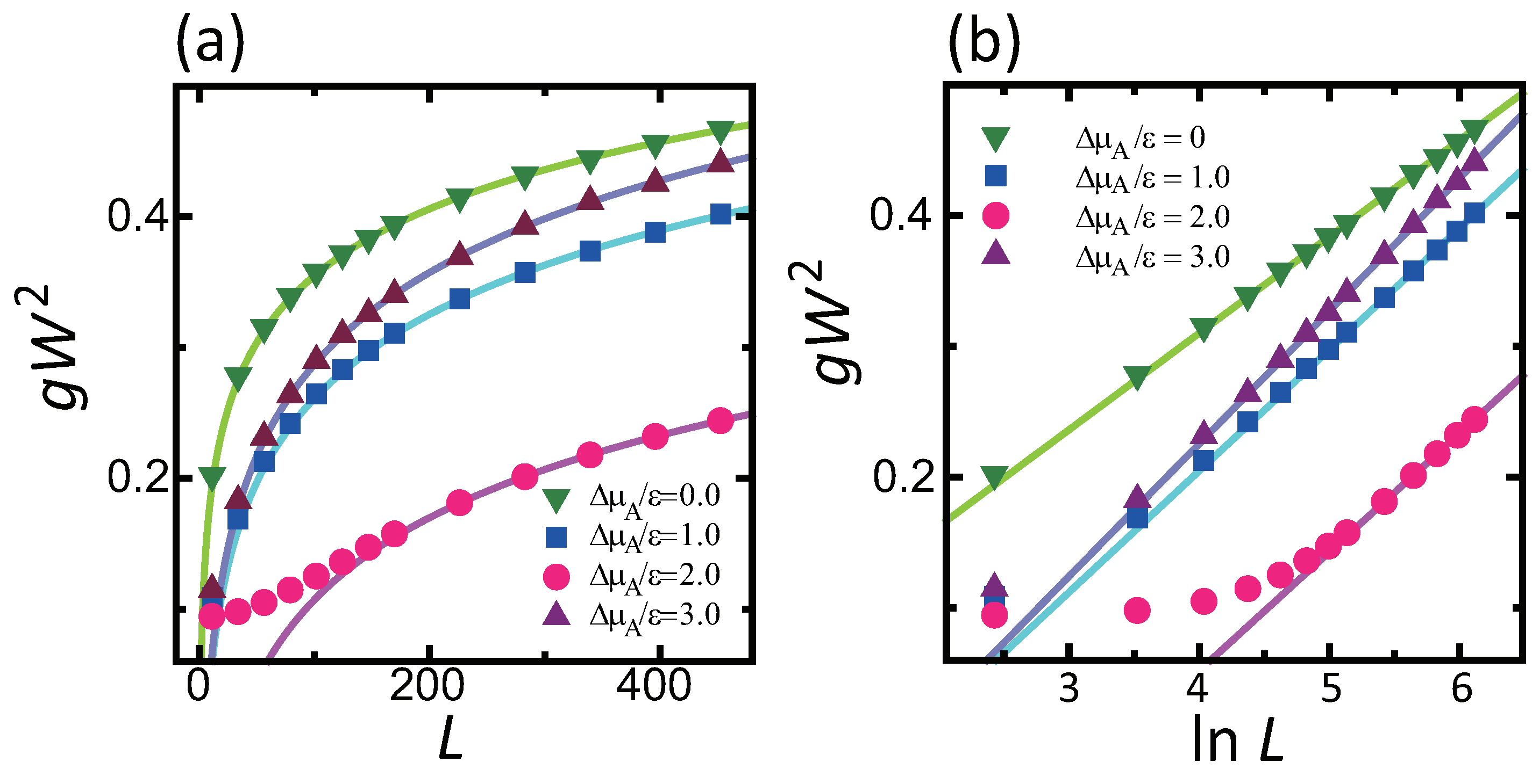
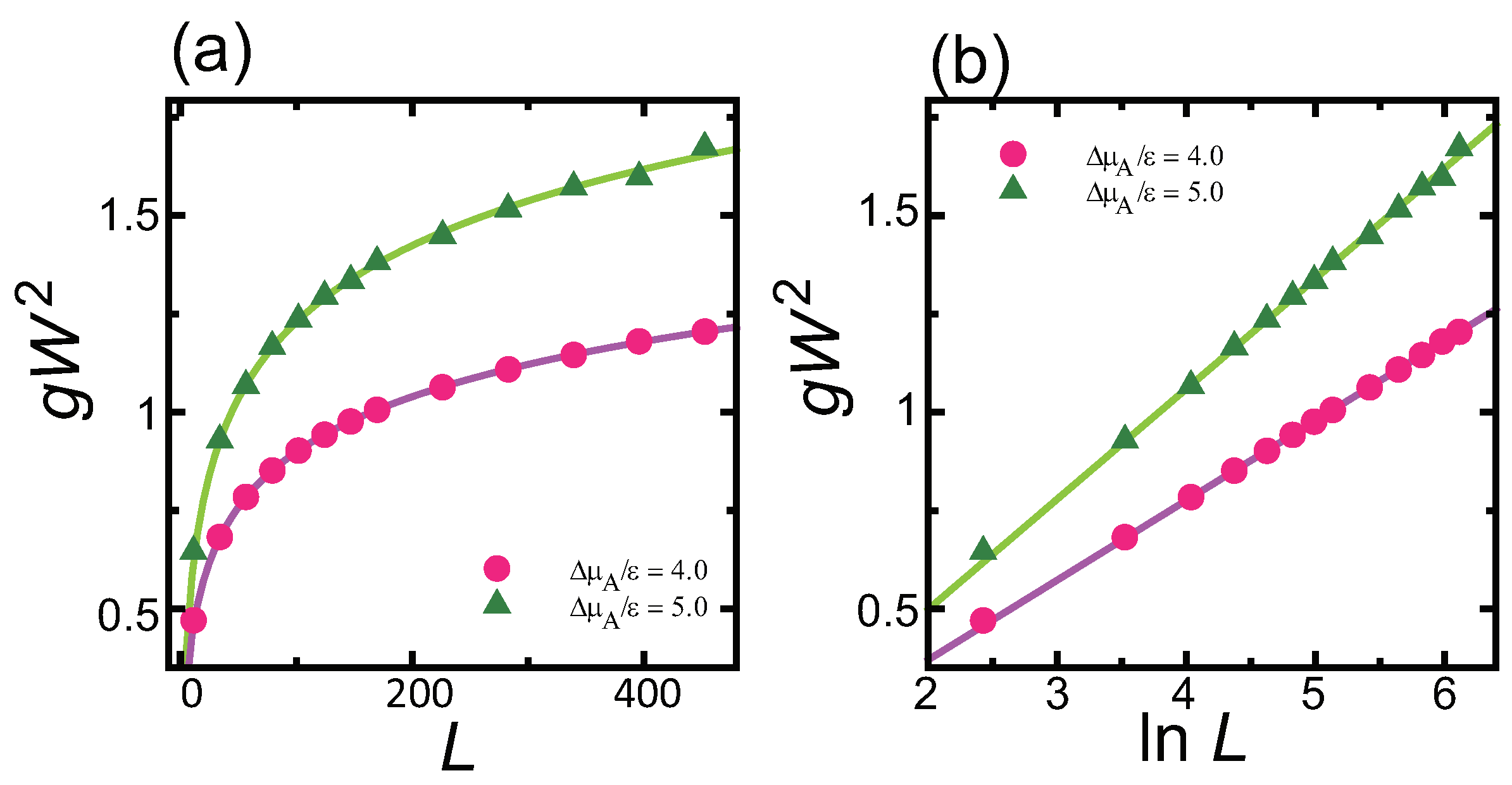
• $\Delta {\mu }_A$ does not affect the roughness exponent; i.e., the roughness exponent $\alpha =0$. For $L>L_{\mathrm{MFL}}$, the squared surface width $W^2(L)$ logarithmically diverges with respect to $L\to \infty$.

The behavior in a small area can be summarized as follows:

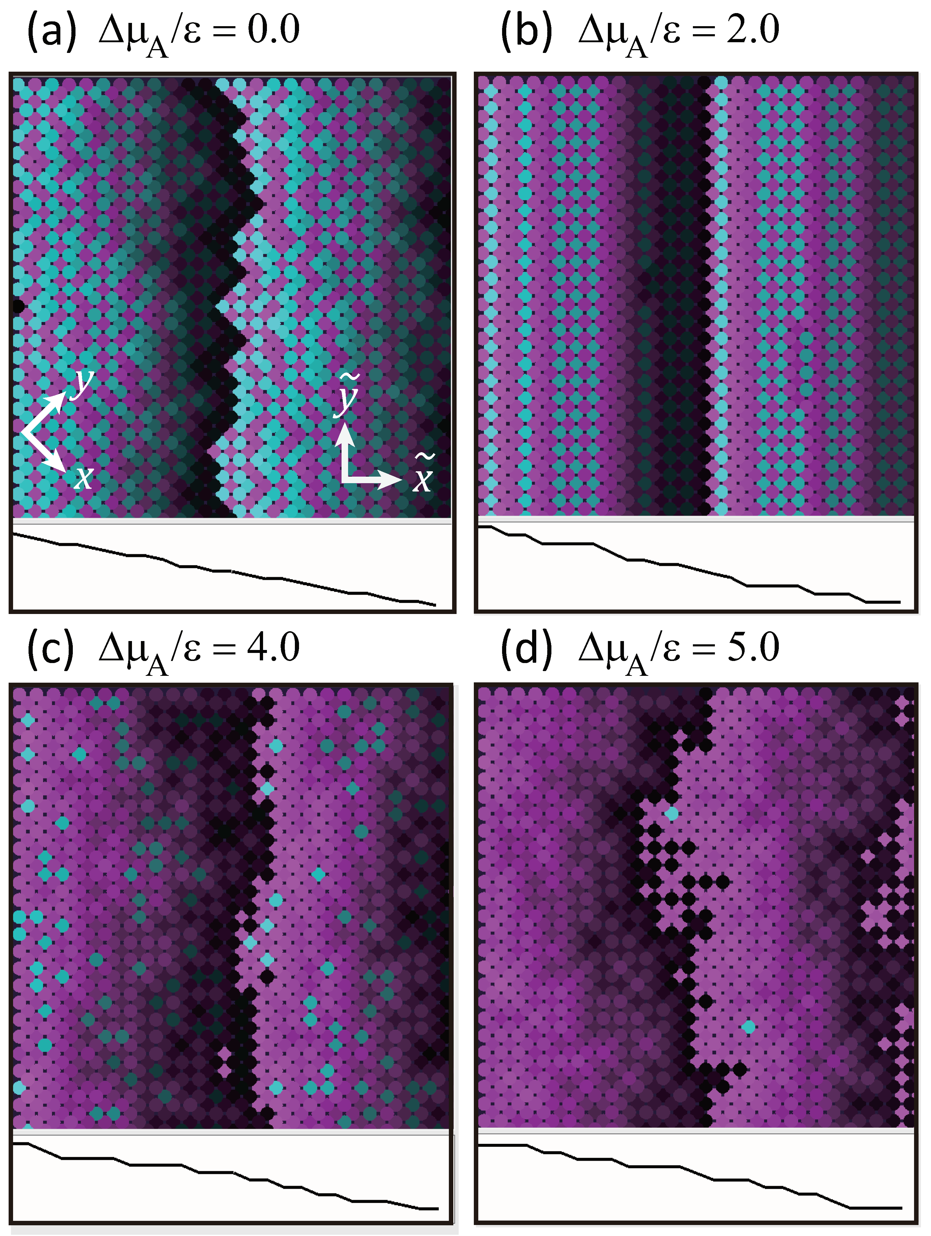
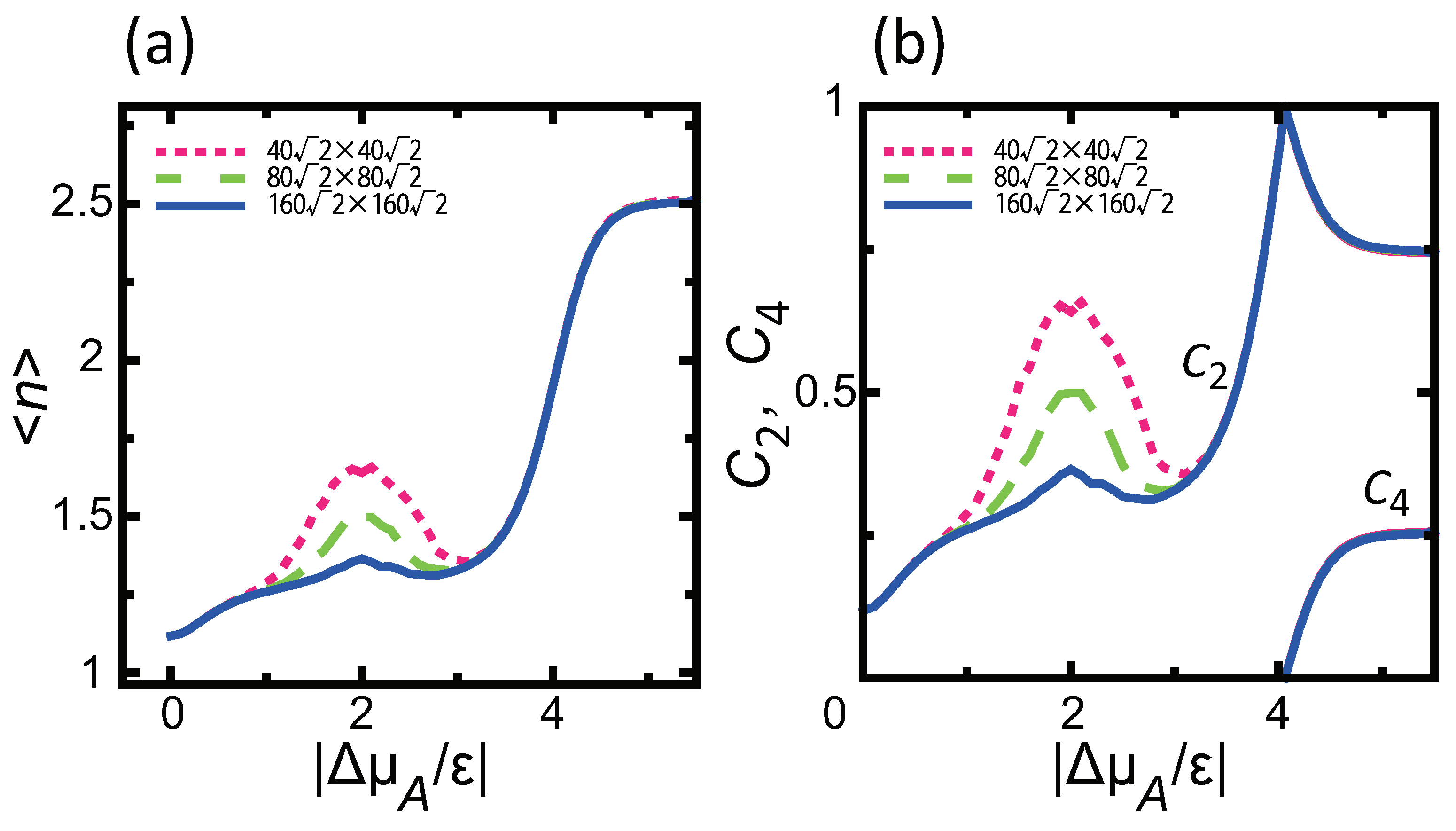
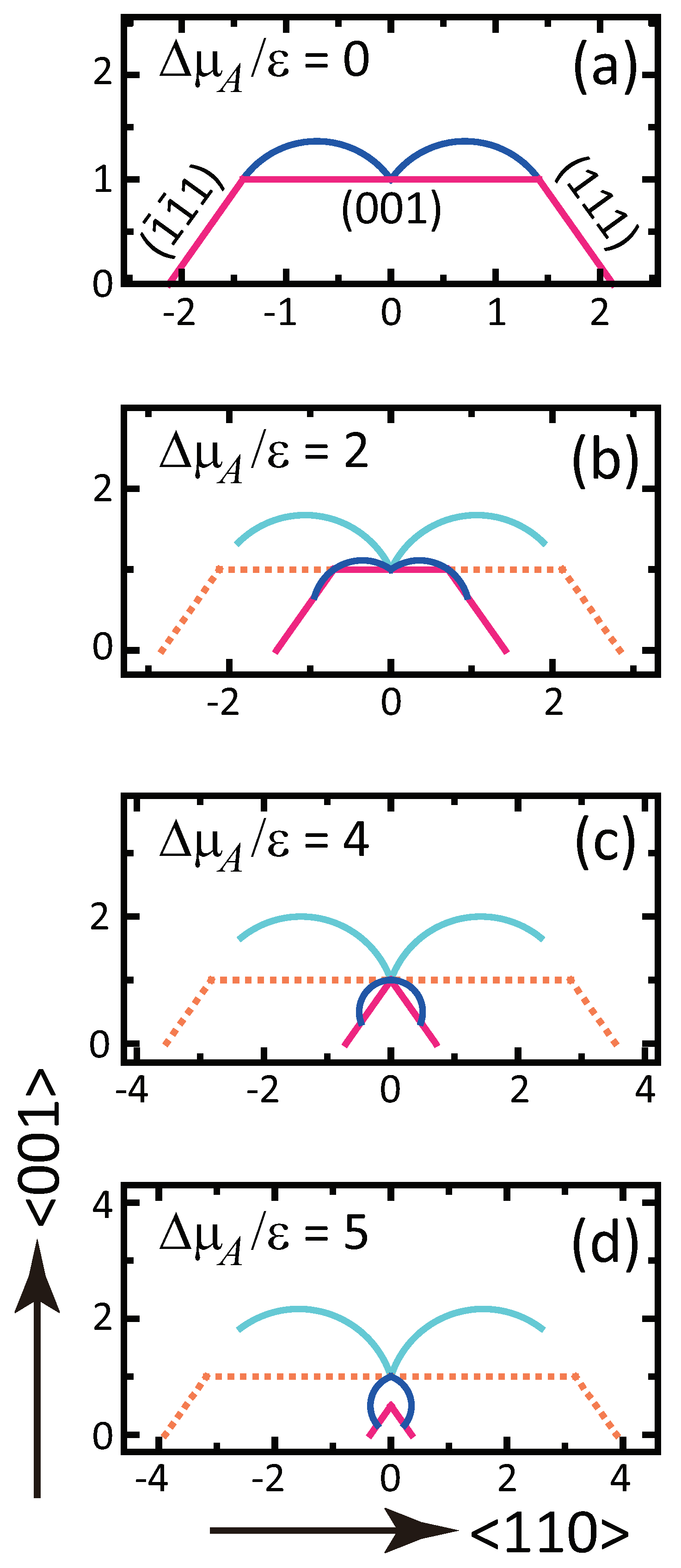
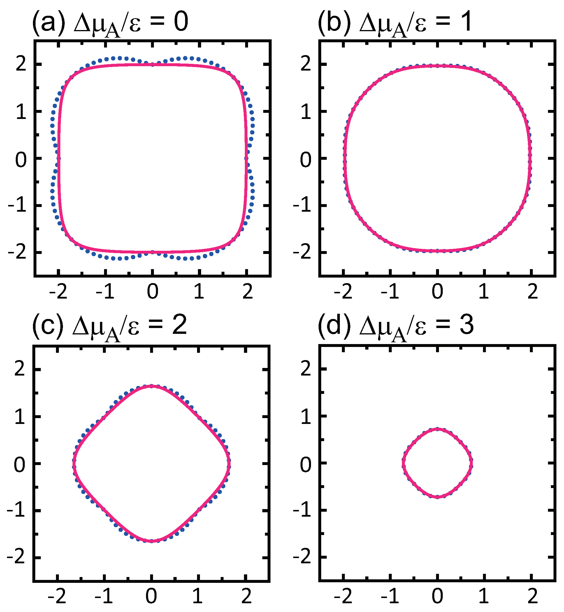
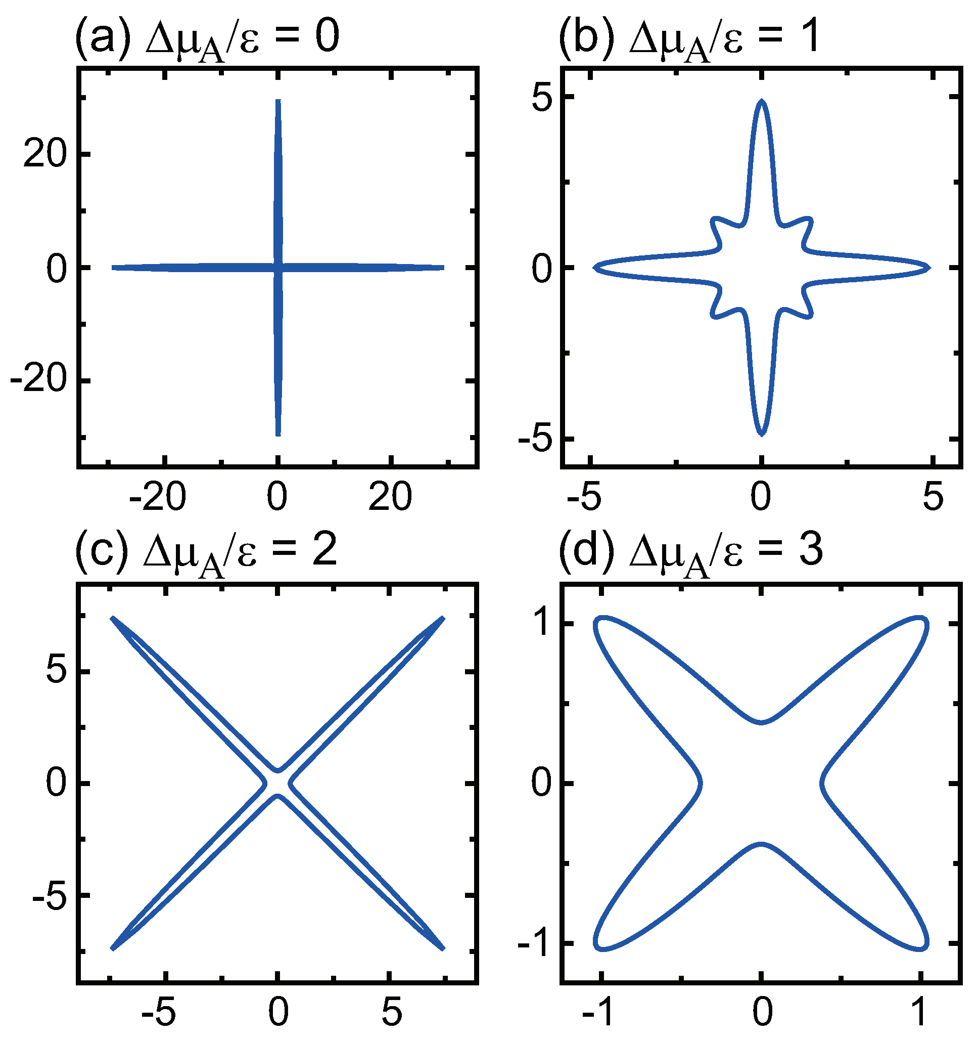
• $\Delta {\mu }_A$ ($\ne 0$) stabilizes polar surfaces by lowering the surface energy. This changes the morphology of the crystal through the anisotropy of the surface tension and step tension. This also causes non-monotonic changes of $g{W}^2$, $\langle n\rangle$, $L_{MFL}$, $\sigma$, and step stiffness with respect to $\Delta {\mu }_A$.
• Double steps and quadruple steps form locally for $|\Delta {\mu }_A/ϵ|\gtrsim 1$ and $|\Delta {\mu }_A/ϵ|\gtrsim 4$, respectively.
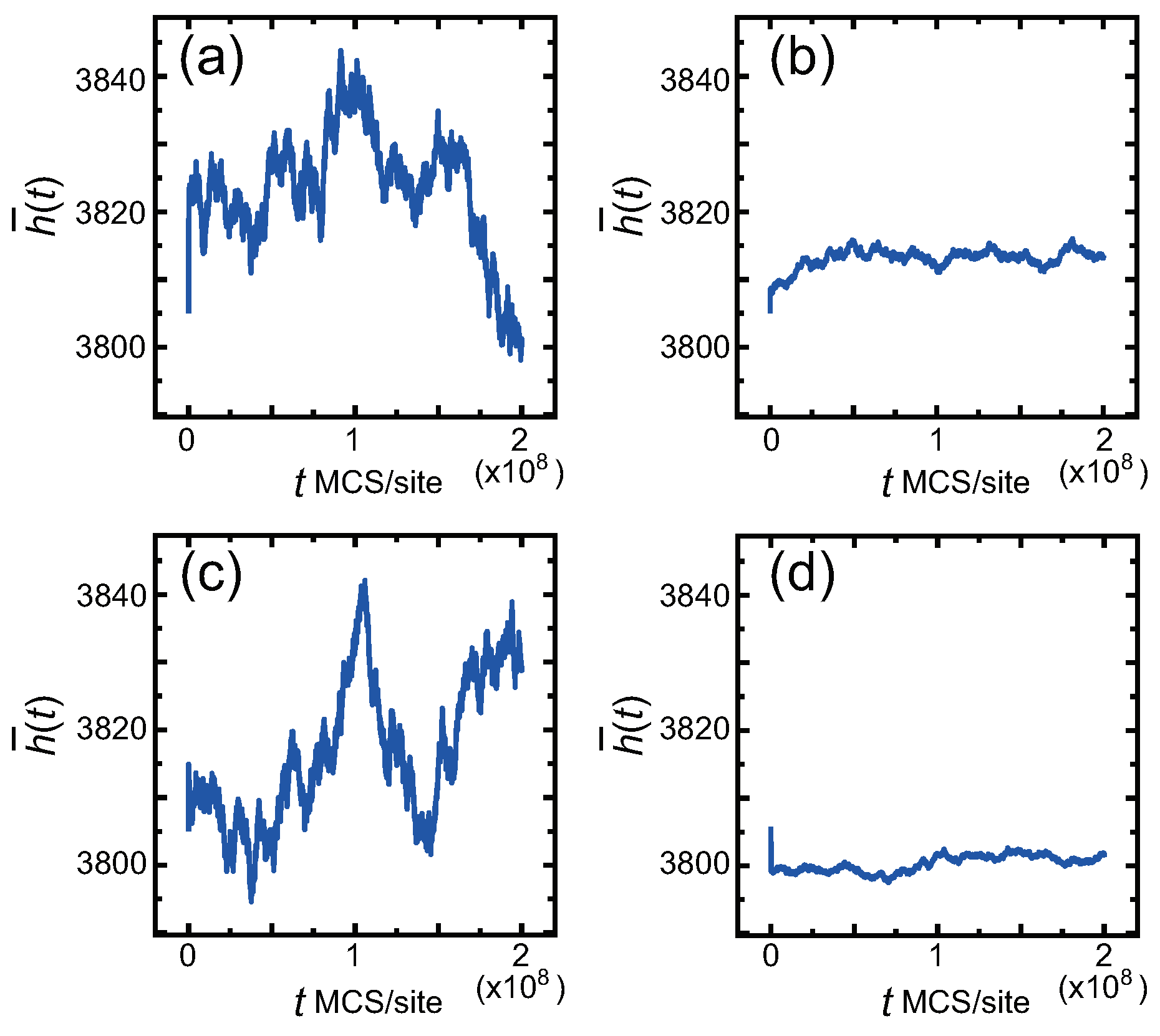
• For $L_{\mathrm{kink}}<L<L_{\mathrm{MFL}}$, $W^2(L)$ is proportional to L; for $L<L_{\mathrm{kink}}$, $W^2(L)$ is constant, making the surface similar to a smooth surface.
• $L_{\mathrm{MFL}}$ is about 160a, where a is the lattice constant, around $|\Delta {\mu }_A/ϵ|=2$. At lower temperatures, $L_{\mathrm{MFL}}$ becomes substantially longer.

The st-RSOS model is a slightly more coarse-grained model compared to that used for the first-principles DFT calculations. This study links the values obtained by first-principles DFT calculations to fundamental quantities required by coarse-grained continuous models on a mesoscopic scale.

References

- Mitani, T.; Komatsu, N.; Takahashi, T.; Kato, T.; Harada, S.; Ujihara, T.; Matsumoto, Y.; Kurashige, K.; Okumura, H. Effect of aluminum addition on the surface step morphology of 4H–SiC grown from Si–Cr–C solution. J. Cryst. Growth 2015, 423, 45–49. [Google Scholar] [CrossRef]
- Akutsu, N. Thermal step bunching on the restricted solid-on-solid model with point contact inter-step attractions. Appl. Surf. Sci. 2009, 256, 1205–1209. [Google Scholar] [CrossRef]
- Akutsu, N. Non-universal equilibrium crystal shape results from sticky steps. J. Phys. Condens. Matter 2011, 23, 485004. [Google Scholar] [CrossRef] [PubMed]
- Akutsu, N. Pinning of steps near equilibrium without impurities, adsorbates, or dislocations. J. Cryst. Growth 2014, 401, 72–77. [Google Scholar] [CrossRef]
- Akutsu, N.; Yamamoto, T. Rough-Smooth Transition of Step and Surface. In Handbook of Crystal Growth; Nishinaga, T., Ed.; Elsevier: London, UK, 2015; Volume I, p. 265. [Google Scholar]
- Einstein, T.L. Equilibrium Shape of Crystals. In Handbook of Crystal Growth; Nishinaga, T., Ed.; Elsevier: London, UK, 2015; Volume I, p. 216. [Google Scholar]
- Akutsu, N. Faceting diagram for sticky steps. AIP Adv. 2016, 6, 035301. [Google Scholar] [CrossRef]
- Akutsu, N. Effect of the roughening transition on the vicinal surface in the step droplet zone. J. Cryst. Growth 2017, 468, 57–62. [Google Scholar] [CrossRef]
- Akutsu, N. Profile of a Faceted Macrostep Caused by Anomalous Surface Tension. Adv. Condens. Matter Phys. 2017, 2017, 2021510. [Google Scholar] [CrossRef]
- Akutsu, N. Sticky steps inhibit step motions near equilibrium. Phys. Rev. E 2012, 86, 061604. [Google Scholar] [CrossRef]
- Akutsu, N. Disassembly of Faceted Macrosteps in the Step Droplet Zone in Non-Equilibrium Steady State. Crystals 2017, 7, 42. [Google Scholar] [CrossRef]
- Akutsu, N. Height of a faceted macrostep for sticky steps in a step-faceting zone. Phys. Rev. Mater. 2018, 2, 023603. [Google Scholar] [CrossRef]
- Akutsu, N. Relationship Between Macrostep Height and Surface Velocity for a Reaction-Limited Crystal Growth Process. Cryst. Growth Des. 2019, 19, 2970–2978. [Google Scholar] [CrossRef]
- Williams, E.D.; Phaneuf, R.J.; Wei, J.; Bartelt, N.C.; Einstein, T.L. Thermodynamics and statistical mechanics of the faceting of stepped Si (111). Surf. Sci. 1993, 294, 219–242, Erratum to “Thermodynamics and statistical mechanics of the faceting of stepped Si (111)” [Surf. Sci. 1993, 294, 219], Surf. Sci. 1994, 310, 451. [Google Scholar] [CrossRef]
- Burton, W.K.; Cabrera, N.; Frank, F.C. The growth of crystals and the equilibrium structure of their surfaces. Philos. Trans. R. Soc. Lond. A 1951, 243, 299–358. [Google Scholar]
- Weeks, J.D.; Gilmer, G.H.; Leamy, H.J. Structural Transition in the Ising-Model Interface. Phys. Rev. Lett. 1973, 20, 549–551. [Google Scholar] [CrossRef]
- Chui, S.T.; Weeks, J.D. Phase transition in the two-dimensional Coulomb gas, and the interfacial roughening transition. Phys. Rev. B 1976, 14, 4978–4982. [Google Scholar] [CrossRef]
- Kosterlitz, J.M.; Thouless, D.J. Ordering, metastability and phase transitions in two-dimensional systems. J. Phys. C 1973, 6, 1181–1203. [Google Scholar] [CrossRef]
- Knops, H.J.F. Exact Relation between the Solid-on-Solid Model and the XY Model. Phys. Rev. Lett. 1977, 39, 766–769. [Google Scholar] [CrossRef]
- Van Beijeren, H. Exactly Solvable Model for the Roughening Transition of a Crystal Surface. Phys. Rev. Lett. 1977, 38, 993–996. [Google Scholar] [CrossRef]
- Weeks, J.D. Ordering in Strongly Fluctuation Condensed Matter Systems; Riste, T., Ed.; Plenum: New York, NY, USA; London, UK, 1980; p. 293. [Google Scholar]
- Jayaprakash, C.; Saam, W.F.; Teitel, S. Roughening and facet formation in crystals. Phys. Rev. Lett. 1983, 50, 2017–2020. [Google Scholar] [CrossRef]
- Rottman, C.; Wortis, M. Equilibrium crystal shapes for lattice models with nearest- and next-nearest-neighbor interactions. Phys. Rev. B 1984, 29, 328–339. [Google Scholar] [CrossRef]
- Rottman, C.; Wortis, M. Statistical mechanics of equilibrium crystal shapes: Interfacial phase diagrams and phase transitions. Phys. Rep. 1984, 103, 59–79. [Google Scholar] [CrossRef]
- Wortis, M. Chemistry and Physics of Solid Surface VII; Vanselow, R., Howe, R., Eds.; Springer: Berlin/Heidelberg, Germany, 1988; pp. 367–405. [Google Scholar]
- Beijeren, V.H.; Nolden, I. Structure and Dynamics of Surfaces; Schommers, W., Blancken-Hagen, V., Eds.; Springer: Berlin/Heidelberg, Germany, 1987; Volume 2, p. 259. [Google Scholar]
- Gruber, E.E.; Mullins, W.W. On the theory of anisotropy of crystalline surface tension. J. Phys. Chem. Solids 1967, 28, 875–887. [Google Scholar] [CrossRef]
- Pokrovsky, V.L.; Talapov, A.L. Ground state, spectrum, and phase diagram of two-dimensional incommensurate crystals. Phys. Rev. Lett. 1979, 42, 65–67. [Google Scholar] [CrossRef]
- Jayaprakash, C.; Rottman, C.; Saam, W.F. Simple model for crystal shapes: Step-step interactions and facet edges. Phys. Rev. B 1984, 30, 6549–6554. [Google Scholar] [CrossRef]
- Akutsu, Y.; Akutsu, N.; Yamamoto, T. Universal jump of Gaussian curvature at the facet edge of a crystal. Phys. Rev. Lett. 1988, 61, 424–427. [Google Scholar] [CrossRef]
- Yamamoto, T.; Akutsu, Y.; Akutsu, N. Universal Behavior of the Equilibrium Crystal Shape near the Facet Edge. I. A Generalized Terrace-Step-Kink Model. J. Phys. Soc. Jpn. 1988, 57, 453–460. [Google Scholar] [CrossRef]
- Mikheev, L.V.; Pokrovsky, V.L. Free-fermion solution for overall equilibrium crystal shape. J. Phys. I 1991, 1, 373–382. [Google Scholar] [CrossRef]
- Huse, D.A.; van Saarloos, W.; Weeks, J.D. Interface Hamiltonians and bulk critical behavior. Phys. Rev. B 1985, 32, 233–246. [Google Scholar] [CrossRef] [PubMed]
- Barabasi, A.L.; Stanley, H.E. Fractal Concepts in Surface Growth; Cambridge University Press: Cambridge, UK, 1995. [Google Scholar]
- Akutsu, N.; Akutsu, Y. Roughening, faceting and equilibrium shape of two-dimensional anisotropic interface. I. Thermodynamics of interface fluctuations and geometry of equilibrium crystal shape. J. Phys. Soc. Jpn. 1987, 56, 1443–1453. [Google Scholar] [CrossRef]
- Yamamoto, T.; Akutsu, Y.; Akutsu, N. Fluctuation of a single step on the vicinal surface-universal and non-universal behaviors. J. Phys. Soc. Jpn. 1994, 63, 915–925. [Google Scholar] [CrossRef]
- Akutsu, Y.; Akutsu, N.; Yamamoto, T. Logarithmic step fluctuations in vicinal surface: A Monte Carlo study. J. Phys. Soc. Jpn. 1994, 63, 2032–2036. [Google Scholar] [CrossRef]
- Takata, M.; Ookawa, A. On the growth mechanism of an A-B crystal. J. Cryst. Growth 1974, 24/25, 515–518. [Google Scholar] [CrossRef]
- Ookawa, A.; Akutsu, N.; Asakura, Y. The growth characteristics of the III-V compound-like crystals affected by the relative activity. In Morphology and Growth Unit of Crystals; Sunagawa, I., Ed.; Terra Scientific Publishing Company: Tokyo, Japan, 1989; pp. 49–50. [Google Scholar]
- Akutsu, N. Equilibrium Crystal Shape of Planar Ising Antiferromagnets in External Fields. J. Phys. Soc. Jpn. 1992, 61, 477–498. [Google Scholar] [CrossRef]
- Nishizawa, S.; Pons, M. Growth and Doping Modeling of SiC–CVD in a Horizontal Hot-Wall Reactor. Chem. Vap. Depos. 2006, 12, 516–522. [Google Scholar] [CrossRef]
- Robertson, N.F.; Jacobsen, J.L.; Saleur, H. Conformally invariant boundary conditions in the antiferromagnetic Potts model and the SL(2,R)/U(1) sigma model. High Energy Phys. 2019, 254, 1–51. [Google Scholar]
- Hsue, C.S.; Lin, K.Y.; Wu, F.Y. Staggered eight-vertex model. Phys. Rev. B 1975, 12, 429–437. [Google Scholar] [CrossRef]
- Kaku, M. Strings, Conformal Fields, and Topology: An Introduction; Springer: New York, NY, USA, 1991. [Google Scholar]
- De Walle, C.G.V.; Neugebauer, J. First-Principles Surface Phase Diagram for Hydrogen on GaN Surfaces. Phys. Rev. Lett. 2002, 88, 066103. [Google Scholar] [CrossRef]
- De Walle, C.G.V.; Neugebauer, J. Structure and energetics of nitride surfaces under MOCVD growth conditions. J. Cryst. Growth 2003, 248, 8–13. [Google Scholar] [CrossRef]
- Akiyama, T.; Yamashita, T.; Nakamura, K.; Ito, T. Stability of hydroben on nonpolar and semipolar nitride surfaces: Role of surface orientation. J. Cryst. Growth 2011, 318, 79–83. [Google Scholar] [CrossRef]
- Kangawa, Y.; Akiyama, T.; Ito, T.; Shiraishi, K.; Nakayama, T. Surface Stability and Growth Kinetics of Compount Semiconductors: An Ab Initio- Based Approach. Materials 2013, 6, 3309–3360. [Google Scholar] [CrossRef]
- Kempisty, P.; Strak, P.; Sakowski, K.; Kangawa, Y.; Krukowski, S. Thermodyamic foundations of application of ab initio methods for determination of the adsorbate equilibria: Hydrogen at the GaN(0001) surface. Phys. Chem. Chem. Phys. 2017, 19, 29676–29684. [Google Scholar] [CrossRef] [PubMed]
- Kempisty, P.; Kangawa, Y. Evolution of the free energy of the GaN(0001) surface based on first-principles phonon calculations. Phys. Rev. B 2019, 100, 085304. [Google Scholar] [CrossRef]
- Krzyzewski, F.; Zaluska-Kotur, M.A. Coexistence of bunching and meandering instability in simulated growth of 4H-SiC(0001) surface. J. Appl. Phys. 2014, 115, 213517. [Google Scholar] [CrossRef]
- Ehrlich, G.; Hudda, F.G. Atomic View of Surface Self-Diffusion: Tungsten on Tungsten. J. Chem. Phys. 1966, 44, 1039. [Google Scholar] [CrossRef]
- Schwoebel, R.L.; Shipsey, E.J. Step Motion on Crystal Surfaces. J. Appl. Phys. 1966, 37, 3682. [Google Scholar] [CrossRef]
- Alerhand, O.L.; Vanderbilt, D.; Meade, R.D.; Joannopoulos, J.D. Spontaneous formation of stress domains on crystal surfaces. Phys. Rev. Lett. 1988, 61, 1973–1976. [Google Scholar] [CrossRef]
- Keshishev, K.O.; Parshin, A.Y.; Babkin, A.V. Crystallization Waves in 4He. Sov. Phys. JETP 1981, 53, 362–369. [Google Scholar]
- Noziéres, P. Liquid and Solid Helium: A Probe of Condensed Matter Phenomena. Phys. Scr. 1987, 1987, 589–593. [Google Scholar] [CrossRef]
- Balibar, S.; Guthmann, C.; Rolley, E. From vicinal to rough crystal surfaces. J. Phys. I 1993, 3, 1475–1491. [Google Scholar] [CrossRef]
- Balibar, S.; Alles, H.; Parshin, A.Y. The surface of helium crystals. Rev. Mod. Phys. 2005, 77, 318–370. [Google Scholar] [CrossRef]
- Abe, H.; Saitoh, Y.; Ueda, T.; Ogasavara, F.; Nomura, R.; Okuda, Y.; Parshin, A.Y. Facet Growth of 4He Crystal Induced by Acoustic Wave. J. Phys. Soc. Jpn. 2006, 75, 023601. [Google Scholar] [CrossRef]
- Nishinaga, T.; Sasaoka, C.; Chernov, A.A. A numerical analysis for the supersaturation distribution around LPE macrostep. Morphology and Growth Unit of Crystals; Sunagawa, I., Ed.; Terra Scientific Publishing Company: Tokyo, Japan, 1989. [Google Scholar]
- Broughton, J.Q.; Gilmer, G.H. Molecular dynamics investigation of the crystal-fluid interface. II. Structures of the fcc (111), (100), and (110) crystal-vapor systems. J. Chem. Phys. 1983, 79, 5105. [Google Scholar] [CrossRef]
- Broughton, J.Q.; Gilmer, G.H. Molecular dynamics investigation of the crystal-fluid interface. III. Dynamical properties of fcc crystal-vapor systems. J. Chem. Phys. 1983, 79, 5119. [Google Scholar] [CrossRef]
- Kangawa, Y.; Ito, T.; Taguchi, A.; Shiraishi, K.; Ohachi, T. A new theoretical approach to adsorption–desorption behavior of Ga on GaAs surfaces. Surf. Sci. 2001, 493, 178–181. [Google Scholar] [CrossRef]
- Widom, B. Statistical Mechanics: A Concise Introduction for Chemists; Cambridge University Press: London, UK, 2002. [Google Scholar]
- Cabrera, N. The equilibrium of crystal surfaces. Surf. Sci. 1964, 2, 320–345. [Google Scholar] [CrossRef]
- Laue, V.M. Der Wulffsche Satz für die Gleichgewichtsform von Kristallen. Z. Kristallogr. 1944, 105, 124–133. [Google Scholar] [CrossRef]
- Herring, C. Some theorems on the free energies of crystal surfaces. Phys. Rev. 1951, 82, 87–93. [Google Scholar] [CrossRef]
- MacKenzie, J.K.; Moore, A.J.W.; Nicholas, J.F. Bonds broken at atomically flat crystal surfaces—I: Face-centred and body-centred cubic crystals. J. Chem. Phys. Solids 1962, 23, 185–196. [Google Scholar] [CrossRef]
- Den Nijs, M. Corrections to scaling and self-duality in the restricted solid-on-solid model. J. Phys. A Math. Gen. 1985, 18, L549–L556. [Google Scholar] [CrossRef]
- Akutsu, N.; Akutsu, Y. Thermal evolution of step stiffness on the Si (001) surface: Temperature-rescaled Ising-model approach. Phys. Rev. B 1998, 57, R4233–R4236. [Google Scholar] [CrossRef]
- Akutsu, N.; Akutsu, Y. The Equilibrium Facet Shape of the Staggered Body-Centered-Cubic Solid-on-Solid Model—A Density Matrix Renormalization Group Study—. Prog. Theor. Phys. 2006, 116, 983–1003. [Google Scholar] [CrossRef]
- Mermin, N.D.; Wagner, H. Absence of ferromagnetism or antiferromagnetism in one-or two-dimensional isotropic Heisenberg models. Phys. Rev. Lett. 1966, 17, 1133–1136, Erratum in 1966, 17, 1307. [Google Scholar] [CrossRef]
- Müller-Krumbhaar, H. Kinetics of crystal growth. In Current Topics in Materials Science; Kaldis, E., Ed.; North-Holland Publishing: Amsterdam, The Nethlands, 1978; Volume 1, Chapter 1; pp. 1–46. [Google Scholar]
- Akutsu, N.; Akutsu, Y. Equilibrium Crystal Shape: Two Dimensions and Three Dimensions. J. Phys. Soc. Jpn. 1987, 56, 2248–2251. [Google Scholar] [CrossRef]
- Akutsu, Y.; Akutsu, N. Interface tension, equilibrium crystal shape, and imaginary zeros of partition function: Planar Ising systems. Phys. Rev. Lett. 1990, 64, 1189–1192. [Google Scholar] [CrossRef] [PubMed]
- Akutsu, N.; Akutsu, Y. An Imaginary Path-Weight Random-Walk Method for Calculation of One-Dimensional Interface Tension. J. Phys. Soc. Jpn. 1990, 59, 3041–3044. [Google Scholar] [CrossRef]
- Akutsu, N.; Akutsu, Y. Step stiffness and equilibrium island shape of Si(100) surface: Statistical-mechanical calculation by the imaginary path weight random-walk method. Surf. Sci. 1997, 376, 92–98. [Google Scholar] [CrossRef]
- Akutsu, N.; Akutsu, Y. Statistical mechanical calculation of anisotropic step stiffness of a two-dimensional hexagonal lattice-gas model with next-nearest-neighbor interactkions: Application to Si(111) surface. J. Phys. Condens. Matter 1999, 11, 6635–6652. [Google Scholar] [CrossRef]
- Akutsu, N. Measurement of microscopic coupling constants between atoms on a surface: Combination of LEEM observation with lattice model analysis. Surf. Sci. 2014, 630, 109–115. [Google Scholar] [CrossRef]
- Bricmont, J.; Lebowitz, J.L.; Pfister, C.E. On the Local Structure of the Phase Separation Line in the Two-Dimensional Ising System. J. Stat. Phys. 1981, 26, 313–332. [Google Scholar] [CrossRef]
- Akutsu, Y.; Akutsu, N. Intrinsic structure of the phase-separation line in the two-dimensional Ising model. J. Phys. A 1987, 20, 5981–5990. [Google Scholar] [CrossRef]
- Akutsu, Y.; Akutsu, N. Relationship between the anisotropic interface tension, the scaled interface width and the equilibrium shape in two dimensions. J. Phys. 1986, A19, 2813–2820. [Google Scholar] [CrossRef]
- Swartzentruber, B.S.; Mo, Y.-W.; Kariotis, R.; Lagally, M.G.; Webb, M.B. Direct determination of step and kink energies on vicinal Si(001). Phys. Rev. Lett. 1990, 65, 1913–1916. [Google Scholar] [CrossRef] [PubMed]
- Swartzentruber, B.S.; Schacht, M. Kinetics of atomic-scale fluctuations of steps on Si (001) measured with variable-temperature STM. Surf. Sci. 1995, 322, 83–89. [Google Scholar] [CrossRef]
- Nozawa, J.; Uda, S.; Guo, S.; Toyotama, A.; Yamanaka, J.; Ihara, N.; Okada, J. Kink Distance and Binding Energy of Colloidal Crystals. Cryst. Growth Des. 2018, 18, 6078–6083. [Google Scholar] [CrossRef]
- Markov, I.V. Crystal Growth for Beginners: Fundamentals of Nucleation, Crystal Growth and Epitaxy, 2nd ed.; World Scientific: Singapore, 2003. [Google Scholar]
- Kashchiev, D. Nucleation: Basic Theory with Applications; Butterworth-Heinemann: Oxford, UK, 2000. [Google Scholar]