Detector Tilt Considerations in Bragg Coherent Diffraction Imaging: A Simulation Study

Abstract

This paper addresses the three-dimensional signal distortion and image reconstruction issues in X-ray Bragg coherent diffraction imaging (BCDI) in the event of a general non-orthogonal orientation of the area detector with respect to the diffracted beam. Growing interest in novel BCDI adaptations at fourth-generation synchrotron light sources has necessitated improvisations in the experimental configuration and the subsequent data analysis. One such possibly unavoidable improvisation that is envisioned in this paper is a photon-counting area detector whose face is tilted away from the perpendicular to the Bragg-diffracted beam during the acquisition of the coherent diffraction signal. We describe a likely circumstance in which one would require such a detector configuration, along with the experimental precedent at third-generation synchrotrons. Using physically accurate diffraction simulations from synthetic scatterers in the presence of such tilted detectors, we analyze the general nature of the observed signal distortion qualitatively and quantitatively and provide a prescription to correct for it during image reconstruction. Our simulations and reconstructions are based on an adaptation of the known theory of BCDI sampling geometry, as well as the recently developed projection-based methods of wavefield propagation. Such configurational modifications and their numerical remedies are potentially valuable in realizing unconventional coherent diffraction measurement geometries, eventually paving the way for the integration of BCDI into new material characterization experiments at next-generation light sources.

1. Introduction

Bragg coherent X-ray diffraction imaging (BCDI) is a synchrotron-based lensless imaging technique for the spatial resolution of lattice distortions on the scale of a few tens of nanometers [1,2,3,4,5,6,7]. BCDI is a valuable means of material characterization owing to its ability to spatially resolve specific components of the 3D lattice strain tensor in deformed crystals, in a nondestructive manner. This is done by reconstructing three-dimensional (3D) real-space images via phase retrieval inversion algorithms [8,9,10,11]. BCDI and the related imaging technique of Bragg ptychography [12,13,14,15,16] together constitute an important set of nano-scale imaging modalities for compact, as well as extended single crystal materials. For instance, BCDI has proven valuable for the imaging of nano-scale driven vortex structures in ferroelectrics [17], inversion domain boundaries in semiconductors [18], and the dynamics of defects and dislocations in energy materials [19,20,21].

With the several orders of magnitude increase in coherent flux at fourth-generation synchrotron light sources (e.g., ESRF-EBS, MAX-IV and the upcoming APS-U), coherent diffraction methods will play an increasingly important role in the 3D characterization of materials’ structure at the nanoscale. The need to incorporate these techniques into existing measurement pipelines will create a requirement for flexible and unconventional diffractometer geometries for the smooth functioning of these multimodal workflows. Such a situation may arise when it is difficult to rotate a conventional detector arm into the required position to query a region of interest in reciprocal space, but BCDI’s capabilities are nevertheless required.

As a concrete example, consider a BCDI measurement interrogating a ferroelectric crystal with fine domain sizes. The structural response of such a material encodes subtle variations in the local polarization (via ion displacement) when viewed on the scale of tens of nanometers, the typical spatial resolution of BCDI. To resolve these variations, one requires the enhanced strain sensitivity of a BCDI measurement at a higher-order Bragg reflection that may well be outside the accessible rotation range of a conventional detector arm. In such a case, one may favor an alternate configuration such as a wall-mounted BCDI detector in which the physical detector chip will not be perpendicular to the exit beam. A recent work exploiting this measurement geometry described the unprecedented nanoscale strain mapping on individual crystalline domains in a poly-grain material by exploiting the partial coherence of a high-energy X-ray beam (52 keV) typically used for meso-scale orientation and strain characterization [22]. The high beam energy necessitated a sample detector distance of ∼7 m in order to resolve diffraction fringes, which was achieved with a BCDI detector mounted along the far wall and whose face was perpendicular to the downstream direction, instead of the diffracted beam (Figure 1).

These examples indicate the possible increasing need for BCDI with unconventional detector configurations at future beamlines.

In anticipation of the increased demand for such BCDI capabilities, this paper addresses the issue of real-space image reconstruction from a BCDI signal distorted by an arbitrary detector orientation. Specifically, we adapt the well-known theory of BCDI coordinate transformations to correctly render a distortion-free 3D image of a synthetic sample (referred to as a scatterer), from a simulated BCDI scan with a tilted detector. The tilt-distorted 3D diffraction pattern is obtained using a customized Fourier transform-based forward propagation model that explicitly takes into account an arbitrary detector tilt. This method draws from the geometric theory of BCDI developed in [23,24] and is demonstrated here with simulations.

It is worth noting that a limited form of this geometric quantification is performed by the xrayutilities software package [25]. Specifically, it addresses the case in which the detector tilt can be decomposed as two independent tilts along the mutually perpendicular sampling directions defined by the pixels. Our work here generalizes this treatment to an arbitrary detector tilt relative to the perpendicular to the exit beam that need not correspond to this decomposition criterion, e.g., when the detector face is rotated about the exit beam. An actual imaging experiment of this kind was performed recently [22], a generalized version of which we illustrate in this paper.

As a recap of the representative experimental schematic [23], we refer to Figure 2, which depicts the following features:

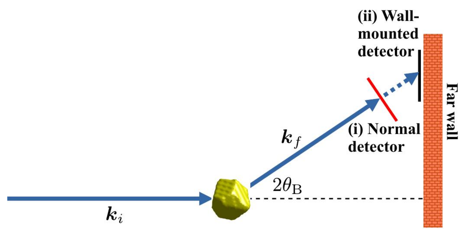
• The scattering geometry with the incident and diffracted wave vectors ${\mathit{k}}_i$ and ${\mathit{k}}_f$, respectively, along with the scattering angle $2{\theta }_B$. ${\mathit{G}}_{hkl}$ is the reciprocal lattice vector corresponding to the active Bragg reflection. Here, $\left|\left|{\mathit{k}}_i\right|\right|=\left|\left|{\mathit{k}}_f\right|\right|=1/\lambda$ in the crystallographers’ convention, where $\lambda$ is the wavelength of the nominally monochromatic X-rays. Their respective directions are given by those of the incident and diffracted beams.
• The orthonormal laboratory frame ${\mathit{B}}_{\mathrm{lab}}=\left[{\widehat{\mathit{s}}}_1{\widehat{\mathit{s}}}_2{\widehat{\mathit{s}}}_3\right]$.
• The orthonormal frame ${\mathit{B}}_{\mathrm{img}}=\left[{\widehat{\mathit{k}}}_1{\widehat{\mathit{k}}}_2{\widehat{\mathit{k}}}_3\right]$, where ${\widehat{\mathit{k}}}_1$ and ${\widehat{\mathit{k}}}_2$ span the plane normal to the exit beam (the “imaging plane”). The direction ${\widehat{\mathit{k}}}_3$ is perpendicular to the imaging plane along the nominal exit beam direction. This is identical to the frame ${\mathit{B}}_{\det }$ from [23].
• The rocking angle $\theta$, in this case about ${\widehat{\mathit{s}}}_2$, but in general about any direction permissible by the experimental arrangement.
• Most importantly, the discrete sampling steps in Fourier space corresponding to the detector pixels, represented as the columns of a $3\times 3$ matrix: ${\mathit{B}}_{\mathrm{recip}}=\left[{\mathit{q}}_i{\mathit{q}}_j{\mathit{q}}_k\right]$. Here, ${\mathit{q}}_i$ and ${\mathit{q}}_j$ are the reciprocal-space steps defined by the pixel dimensions along ${\widehat{\mathit{k}}}_1$ and ${\widehat{\mathit{k}}}_2$. The incremental migration of the 3D diffraction signal through the imaging plane by virtue of the $\theta$ rotation is denoted in this convention by $-{\mathit{q}}_k$ and is independent of the detector pixel dimensions.

The azimuth and elevation angles $\delta$ and $\gamma$ in Figure 2 are specific to the configuration at the 34-ID-C end station of the Advanced Photon Source and denote typical diffractometer-based parameterizations of the detector position. In BCDI, the column vectors of ${\mathit{B}}_{\mathrm{recip}}$ are not mutually orthogonal owing to the geometry of ${\mathit{q}}_k$ ([23] contains a derivation of this fact). However, the detector is typically arranged with its face normal to the exit beam such that ${\mathit{q}}_i\Vert {\widehat{\mathit{k}}}_1$ and ${\mathit{q}}_j\Vert {\widehat{\mathit{k}}}_2$, as seen in Figure 2.

Let the dimensions of the acquired data set be $N_1\times N_2\times N_3$, where $N_1$ and $N_2$ denote the pixel span of the detector and $N_3$ the number of discrete steps in the rocking direction ($\theta$ in Figure 2). The thesis of [23] is: given that ${\mathit{B}}_{\mathrm{recip}}=\left[{\mathit{q}}_i{\mathit{q}}_j{\mathit{q}}_k\right]$ can be computed from the experimental geometry, the real-space sampling steps associated with the three axes of the digital phase-retrieved object may be similarly expressed as the columns of another matrix ${\mathit{B}}_{\mathrm{real}}$. Generally, the mutual non-orthogonality of the columns of ${\mathit{B}}_{\mathrm{real}}$ implies a non-orthogonality in the sampling of the reconstructed 3D object. It has been shown [23] that ${\mathit{B}}_{\mathrm{real}}$ is given by:

$$\begin{array}{cc}\hfill {\mathit{B}}_{\mathrm{real}}& ={\mathit{B}}_{\mathrm{recip}}^{-T}\mathcal{D}\hfill \\ \hfill \mathrm{where}\mathcal{D}& =\left[\begin{array}{ccc}{N}_1^{-1}& & \\ & N_2^{-1}& \\ & & N_3^{-1}\end{array}\right]\hfill \end{array}$$

(1)

and $-T$ equivalently denotes the inverse of the transpose or the transpose of the inverse.

The phase-retrieved array containing the real-space scatterer, combined with the knowledge of the shear encoded in ${\mathit{B}}_{\mathrm{real}}$, is sufficient for accurate, undistorted rendering of the scatterer with one of several available software packages for 3D visualization. For the interested reader, the method to directly compute gradients on a grid of such sheared sample points (required to convert the scatterer’s complex phase to a spatially resolved lattice strain field) is provided in the Appendix of [23].

2. A Tilted Detector

The shear-correcting coordinate inversion method summarized in Section 1 generalizes to any BCDI configuration provided the sampling basis matrix ${\mathit{B}}_{\mathrm{recip}}$ is properly parameterized according to the experimental degrees of freedom. The detector plane was assumed perpendicular to the exit beam, an arrangement typically ensured in BCDI by fixing the detector on a radial arm, facing inwards and pointed directly at the mounted scatterer (Case (i) in Figure 1). In this section, we demonstrate the flexibility of the sampling basis formalism of Equation (1) in addressing the general case when ${\mathit{q}}_i$ and ${\mathit{q}}_j$ are not aligned parallel to ${\widehat{\mathit{k}}}_1$ and ${\widehat{\mathit{k}}}_2$, respectively. As demonstrated in [22], such a situation may arise in the design of future BCDI facilities in which the detector configuration is dictated not by diffractometer rotations such as $\gamma$ and $\delta$, but relatively inexpensive translation stages, an example of which is shown in Figure 1, Case (ii). Such a modification would greatly simplify the design of a BCDI measurement, with the burden of correcting for the tilt-induced signal distortion being placed on numerical methods.

We first consider a simplifying assumption. We assume an ideal detector with pixels capable of perfect response, which faithfully register an incident photon in its entirety. We further assume that the pixels are not susceptible to energy redistribution due to the passage of the incident radiation through multiple adjacent pixels owing to the slanted propagation path [26]. This undesirable feature of real-world detectors would result in a blurring effect of the acquired signal whose correction, while in principle addressable as an additional deconvolution problem, could involve the details of detector chip design, thereby complicating the image reconstruction process. Numerical corrections to address this blurring issue are detector-specific and therefore outside the scope of this work.

We now refer to the schematic in Figure 3. In Figure 3a, we see a simplified one-dimensional detector arranged to capture the peak of a Bragg reflection at its center, but tilted away from the imaging plane by an angle $\xi$. Here, we denote the distance between the object and the center of the detector as L and the pixel pitch as p. This arrangement renders the extent of angular space queried by the detector smaller by a factor of $cos\xi$ (note the region of angular information “lost” to the BCDI measurement). The Fourier space norm of the pixel step is no longer $p/\lambda L$, as shown in [23], but $(p/\lambda L)cos\xi$. The scattered intensity in the region of lost information does not contribute to the acquired signal. Even in the case of a high signal-to-noise ratio (SNR), this would result in a measurement with missing higher order Fourier components and therefore a reconstruction with necessarily lower spatial resolution. A more general treatment of this one-dimensional detector case is found in [25].

We wish to generalize this idea to the case of a two-dimensional area detector arbitrarily tilted with respect to the exit beam. We refer to Figure 3b, in which the diffraction signal within the blue outline depicts what would be measured if the detector face were aligned with the imaging plane (i.e., the plane of the figure). The exit beam ${\mathit{k}}_f$ enters the imaging plane perpendicular to the figure. Shown also is the projection of the detector face if it were tilted arbitrarily (red outline), effectively a sheared window when viewed along the exit beam. The region of lost signal information is now the area in between the blue and red quadrilaterals.

We first define the mutually perpendicular sampling steps ${\mathit{q}}_i^{\left(\mathrm{tilt}\right)}$ and ${\mathit{q}}_j^{\left(\mathrm{tilt}\right)}$ as fixed to the physical pixels of the area detector, which rotate along with the detector as it is tilted away from the imaging plane. For a normal detector, this definition of ${\mathit{q}}_{i,j}^{\left(\mathrm{tilt}\right)}$ coincides with that of ${\mathit{q}}_{i,j}$ from [23]. For a tilted detector, these vectors no longer lie in the imaging plane, and we now seek their respective projections ${\mathit{q}}_i^{\prime }$ and ${\mathit{q}}_j^{\prime }$ in the imaging plane, akin to the situation in Figure 3a. Owing to the arbitrary detector tilt, the projections $\{{\mathit{q}}_i^{\prime },{\mathit{q}}_j^{\prime }\}$ are not orthogonal in general, even though they still span the imaging plane. The projection operator $\mathit{P}$ into the imaging plane is a $3\times 3$ matrix defined by:

$$\mathit{P}=\mathcal{I}-{\widehat{\mathit{k}}}_3{\widehat{\mathit{k}}}_3^T$$

(2)

where $\mathcal{I}$ is the $3\times 3$ identity matrix and ${\widehat{\mathit{k}}}_3$ is the third axis of the detector frame (along the direction of the exit beam), treated as a $3\times 1$ column vector. With this, we can compute the effective sampling steps in the imaging plane:

$$\begin{array}{c}\hfill {\mathit{q}}_i^{\prime }=\mathit{P}{\mathit{q}}_i^{\left(\mathrm{tilt}\right)}\end{array}$$

(3)

$$\begin{array}{c}\hfill {\mathit{q}}_j^{\prime }=\mathit{P}{\mathit{q}}_j^{\left(\mathrm{tilt}\right)}\end{array}$$

(4)

The basis vectors ${\mathit{q}}_i$ and ${\mathit{q}}_j$ in the matrix expression for ${\mathit{B}}_{\mathrm{recip}}$ are respectively replaced by ${\mathit{q}}_i^{\prime }$ and ${\mathit{q}}_j^{\prime }$ from Equations (3) and (4). The modified ${\mathit{B}}_{\mathrm{recip}}$ in turn allows us to calculate the correct ${\mathit{B}}_{\mathrm{real}}$ according to Equation (1).

We note the following:

• The third sampling vector ${\mathit{q}}_k$ is not modified by the tilt of the detector, since it depends only on the Bragg reflection of interest and the direction of scatterer rocking.
• The information of the detector tilt is introduced into ${\mathit{q}}_i^{\prime }$ and ${\mathit{q}}_j^{\prime }$ not through the projection operator $\mathit{P}$, but the now out-of-plane vectors ${\mathit{q}}_i^{\left(\mathrm{tilt}\right)}$ and ${\mathit{q}}_j^{\left(\mathrm{tilt}\right)}$.
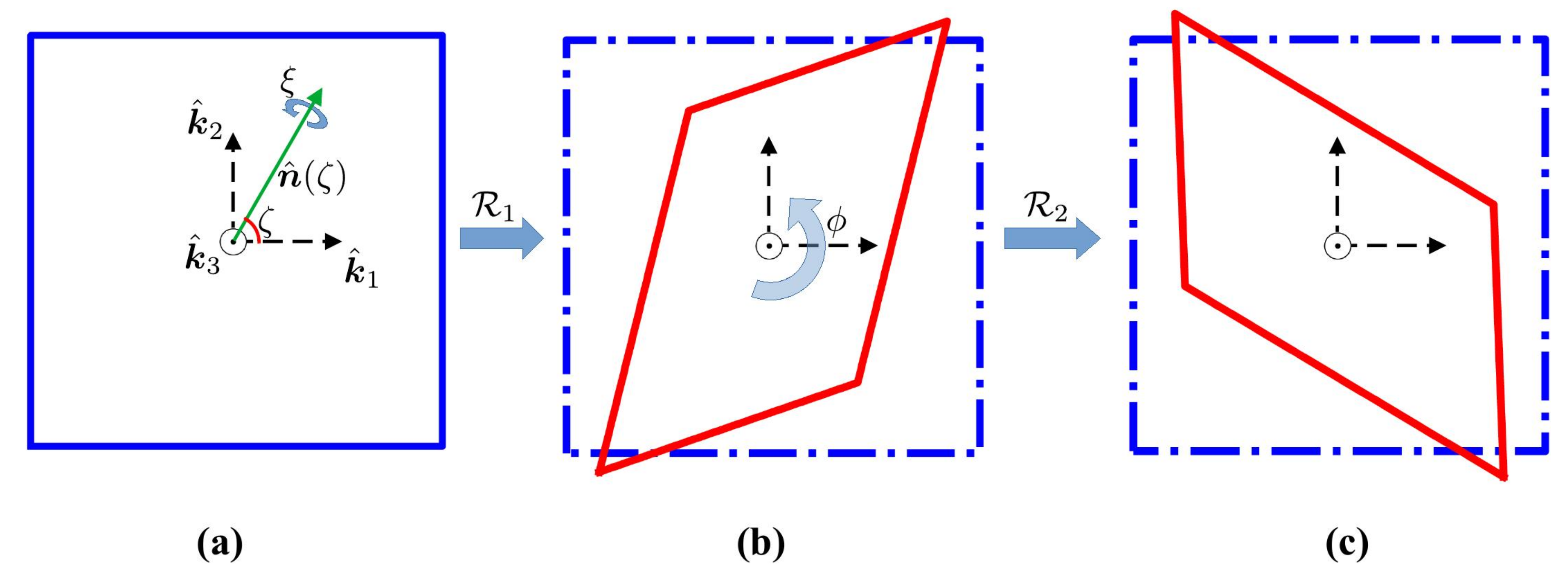
• As seen in Figure 3c, a tilted detector results in the measurements of a distorted diffraction pattern ${\left|\left|{\mathsf{\Psi }}^{\prime }\left(\mathit{q}\right)\right|\right|}^2$, which in turn corresponds to the distorted wave field ${\mathsf{\Psi }}^{\prime }\left(\mathit{q}\right)e^{\iota 2\pi {\mathit{C}}_0^T\mathit{q}}$. Here, ${\mathsf{\Psi }}^{\prime }\left(\mathit{q}\right)$ denotes the wave field resulting from the in-plane distortion, while the complex exponential phase ramp $e^{\iota 2\pi {\mathit{C}}_0^T\mathit{q}}$ parameterized by a constant vector ${\mathit{C}}_0$ denotes the distribution of the phase lag in the interrogated wave field relative to the phase profile at the imaging plane. This additional linearly varying phase clearly does not influence the measured signal and is therefore not considered from here on, assuming the measurements are in fact made in the far-field regime.

3. Simulation Results

We now demonstrate the reconstruction of a synthetic digital object from simulated BCDI scans acquired at various detector tilts. For all the following simulations, we adopt the self-conjugate detector frame ${\mathit{B}}_{\mathrm{img}}=\left[{\widehat{\mathit{k}}}_1{\widehat{\mathit{k}}}_2{\widehat{\mathit{k}}}_3\right]$ defined earlier in which to render the original and reconstructed objects, as well as the Fourier-space signal. For simplicity, the synthetic object in question is a phase-less pyramid with a square base, with well-defined facets and edges. The forward model to simulate the signal acquired using tilted detectors is described in detail in Appendix A, along with a summary of the various detector tilts used in the simulations. These manipulations are predicated upon the projection-based far-field propagation method, whose detailed derivation was the subject of [24]. Here, in the interest of highlighting the detector tilt-induced object shear and its correction, we bypass the phase retrieval process altogether and merely obtain the “reconstructions” of the scatterer from the inverse FFT of the simulated wave fields, then compare their morphologies before and after the distortions that arise from Equations (3) and (4) having been corrected. Under these circumstances, the inverse FFT is simply a proxy for the phase retrieval solution in the limit of an infinite signal-to-noise ratio.

Figure 4 shows the simulated diffraction signals of the phase-less pyramid that has been arbitrarily oriented in the detector frame, when the detector is tilted in different ways with respect to the exit beam. We note the “stretched” nature of the diffraction patterns in Figure 4b–e along various directions owing to the tilted detector, when compared to the diffraction pattern in Figure 4a (corresponding to the perpendicular detector). For example, Figure 4b shows the diffraction when the detector is tilted by ${60}^{\circ }$ about ${\widehat{\mathit{k}}}_1$, which appears like the diffraction pattern in Figure 4a, but stretched along ${\widehat{\mathit{k}}}_2$. This signal contains corrupted high-frequency fringe information along this direction, which in a real-world measurements would translate to a deficiency of spatial resolution that would manifest in the blurred edges of the reconstructed object. Similarly, Figure 4c shows the signal when the detector is rotated by ${60}^{\circ }$ about ${\widehat{\mathit{k}}}_2$ (i.e., $\xi ={60}^{\circ }$, $\zeta ={90}^{\circ }$), resulting in a stretch along ${\widehat{\mathit{k}}}_1$ and a corresponding blurring along the edges of the recovered object. Figure 4 also show the distorted diffraction signal in the case of more complicated detector tilts (see Appendix A for a full summary). In each row, the second and third images show the amplitude and phase cross-sections of the recovered object with a simple inverse FFT of the diffracted wave field. This is what would have been recovered in an actual phase retrieval reconstruction.

In each case, the tilt-corrected pyramid isosurface is shown along with the corresponding isosurface when one disregards the detector tilt (fourth and fifth images in each row, respectively). More specifically, the fourth image in each row corresponds to the correct real-space sampling basis ${\mathit{B}}_{\mathrm{real}}$, obtained from Equation (1) after properly accounting for the detector tilt (the tilt corrections in each case being given by Equations (3) and (4)). The fifth image in each row of Figure 4 corresponds to the inferred object without accounting for the detector tilt. Clearly, the tilt-corrected isosurface agrees with the original pyramid in Figure 4a in terms of morphology and orientation.

It was observed that phase variation in the interior of the (nominally phase-less) recovered object following the forward propagation was insignificant, ∼${10}^{-4}$ radians (see the Jupyter notebook in the Supplementary Material). Further, we note that Figure 4e corresponds to the area detector being rotated by ${73}^{\circ }$ about the exit beam direction ${\widehat{\mathit{k}}}_3$. In contrast, the xrayutilities formalism assumes a conventional “3S + 2D” goniometer configuration (three sample rotations, two detector rotations with the detector nominally fixed perpendicular to the exit beam) and corrects for small rotations of the detector about the exit beam direction. In this sense, the rotation of ${73}^{\circ }$ is outside the scope of analysis by xrayutilities.

We also note that the detector tilt angle of ∼${14}^{\circ }$ in Figure 4f may correspond to a realistic measurement similar to that described in [22] with a wall-mounted detector. This follows from the fact that the tilt of a wall-mounted detector is equal to the scattering angle $2{\theta }_{\mathrm{B}}$ (as can be seen from Figure 1’s schematic). The scattering angle in turn corresponds to a number of higher order Bragg reflections from a crystal whose lattice constant is similar to crystalline gold ($4.078$ Å), measured with a coherent beam of energy 40 keV. The tilt angles of ${60}^{\circ }$ and ${91}^{\circ }$, on the other hand, do not necessarily correspond to a conceivable BCDI measurement. Nevertheless, they represent valid points in the continuous space of detector tilts. They have been included here to illustrate the robust generalizability of the sampling basis formulation to very large and seemingly unwieldy tilts.

The striations on the pyramid faces in Panels (b) through (f) can also be explained by the corruption of the high-frequency Fourier components caused by cyclic aliasing in the simulation process. In a real-world measurement with a tilted detector, the high-frequency Fourier components are not aliased, but genuinely lost to the measurement because they fall outside the aperture defined by the projected area of the detector (see Figure 3b). In general, this results in a loss of spatial resolution in the reconstructed object.

4. Conclusions

We derive a geometric correction for the morphology of a reconstructed scatterer in a BCDI measurement with a detector tilted with respect to the diffracted beam. The correction method demonstrated is seen to be a straightforward generalization of the mathematical theory developed in [23]. We successfully validate our theory by developing a customized forward model of the distorted diffraction signal acquired by a tilted detector and adapting the coordinate transform theory from [23] to obtain the correct post-phase retrieval 3D rendering of the original object. The detector tilt angles in our simulations are chosen primarily in order to illustrate the completely generalizable nature of the sampling basis formalism from Equation (1) in describing signal distortion. The geometric manipulations described in this paper guarantees accurate reconstructability regardless of the tilt angle. Thereby, we demonstrate potential flexibility in physical BCDI experiment design by offloading the computational burden of inverting a distorted signal to numerical methods.

References

1. Robinson, I.K.; Vartanyants, I.A.; Williams, G.J.; Pfeifer, M.A.; Pitney, J.A. Reconstruction of the Shapes of Gold Nanocrystals Using Coherent X-ray Diffraction. Phys. Rev. Lett. 2001, 87, 195505. [Google Scholar] [CrossRef] [Green Version]
2. Williams, G.; Pfeifer, M.; Vartanyants, I.; Robinson, I. Three-dimensional imaging of microstructure in Au nanocrystals. Phys. Rev. Lett. 2003, 90, 175501. [Google Scholar] [CrossRef] [PubMed] [Green Version]
3. Pfeifer, M.A.; Williams, G.J.; Vartanyants, I.A.; Harder, R.; Robinson, I.K. Three-dimensional mapping of a deformation field inside a nanocrystal. Nature 2006, 442, 63–66. [Google Scholar] [CrossRef] [PubMed]
4. Williams, G.; Pfeifer, M.; Vartanyants, I.; Robinson, I. Internal structure in small Au crystals resolved by three-dimensional inversion of coherent X-ray diffraction. Phys. Rev. B 2006, 73, 094112. [Google Scholar] [CrossRef] [Green Version]
5. Newton, M.C.; Leake, S.J.; Harder, R.; Robinson, I.K. Three-dimensional imaging of strain in a single ZnO nanorod. Nat. Mater. 2010, 9, 120–124. [Google Scholar] [CrossRef]
6. Harder, R.; Liang, M.; Sun, Y.; Xia, Y.; Robinson, I. Imaging of complex density in silver nanocubes by coherent X-ray diffraction. New J. Phys. 2010, 12, 035019. [Google Scholar] [CrossRef]
7. Newton, M.C.; Harder, R.; Huang, X.; Xiong, G.; Robinson, I.K. Phase retrieval of diffraction from highly strained crystals. Phys. Rev. B 2010, 82, 165436. [Google Scholar] [CrossRef]
8. Fienup, J.R. Phase retrieval algorithms: A comparison. Appl. Opt. 1982, 21, 2758–2769. [Google Scholar] [CrossRef] [Green Version]
9. Fienup, J.R.; Wackerman, C.C. Phase-retrieval stagnation problems and solutions. J. Opt. Soc. Am. A 1986, 3, 1897–1907. [Google Scholar] [CrossRef]
10. Zhang, F.; Chen, B.; Morrison, G.R.; Vila-Comamala, J.; Guizar-Sicairos, M.; Robinson, I.K. Phase retrieval by coherent modulation imaging. Nat. Commun. 2016, 7, 1–8. [Google Scholar] [CrossRef] [Green Version]
11. Guizar-Sicairos, M.; Fienup, J.R. Phase retrieval with transverse translation diversity: A nonlinear optimization approach. Opt. Express 2008, 16, 7264–7278. [Google Scholar] [CrossRef]
12. Godard, P.; Carbone, G.; Allain, M.; Mastropietro, F.; Chen, G.; Capello, L.; Diaz, A.; Metzger, T.H.; Stangl, J.; Chamard, V. Three-dimensional high-resolution quantitative microscopy of extended crystals. Nat. Commun. 2011, 2, 1–6. [Google Scholar] [CrossRef]
13. Hruszkewycz, S.; Holt, M.; Murray, C.; Bruley, J.; Holt, J.; Tripathi, A.; Shpyrko, O.; McNulty, I.; Highland, M.; Fuoss, P. Quantitative nanoscale imaging of lattice distortions in epitaxial semiconductor heterostructures using nanofocused X-ray Bragg projection ptychography. Nano Lett. 2012, 12, 5148–5154. [Google Scholar] [CrossRef]
14. Pateras, A. Three Dimensional X-ray Bragg Ptychography of an Extended Semiconductor Heterostructure. Ph.D. Thesis, Aix Marseille University, Marseille, France, 2015. [Google Scholar]
15. Hruszkewycz, S.O.; Allain, M.; Holt, M.V.; Murray, C.E.; Holt, J.R.; Fuoss, P.H.; Chamard, V. High-resolution three-dimensional structural microscopy by single-angle Bragg ptychography. Nat. Mater. 2017, 16, 244–251. [Google Scholar] [CrossRef] [Green Version]
16. Hill, M.O.; Calvo-Almazan, I.; Allain, M.; Holt, M.V.; Ulvestad, A.; Treu, J.; Koblmuller, G.; Huang, C.; Huang, X.; Yan, H.; et al. Measuring Three-Dimensional Strain and Structural Defects in a Single InGaAs Nanowire Using Coherent X-ray Multiangle Bragg Projection Ptychography. Nano Lett. 2018, 18, 811–819. [Google Scholar] [CrossRef] [Green Version]
17. Karpov, D.; Liu, Z.; Rolo, T.d.S.; Harder, R.; Balachandran, P.V.; Xue, D.; Lookman, T.; Fohtung, E. Three-dimensional imaging of vortex structure in a ferroelectric nanoparticle driven by an electric field. Nat. Commun. 2017, 8, 280. [Google Scholar] [CrossRef]
18. Labat, S.; Richard, M.I.; Dupraz, M.; Gailhanou, M.; Beutier, G.; Verdier, M.; Mastropietro, F.; Cornelius, T.W.; Schülli, T.U.; Eymery, J.; et al. Inversion Domain Boundaries in GaN Wires Revealed by Coherent Bragg Imaging. ACS Nano 2015, 9, 9210–9216. [Google Scholar] [CrossRef]
19. Ulvestad, A.; Singer, A.; Clark, J.; Cho, J.; Kim, J.W.; Harder, R.; Maser, J.; Meng, S.; Shpyrko, O. Topological Defect Dynamics in Operando Battery Nanoparticles. Science 2015, 348, 1344–1347. [Google Scholar] [CrossRef] [Green Version]
20. Ulvestad, A.; Welland, M.J.; Cha, W.; Liu, Y.; Kim, J.W.; Harder, R.; Maxey, E.; Clark, J.N.; Highland, M.J.; You, H.; et al. Three-dimensional imaging of dislocation dynamics during the hydriding phase transformation. Nat. Mater. 2017, 16, 565–571. [Google Scholar] [CrossRef]
21. Singer, A.; Zhang, M.; Hy, S.; Cela, D.; Fang, C.; Wynn, T.A.; Qiu, B.; Xia, Y.; Liu, Z.; Ulvestad, A.; et al. Nucleation of dislocations and their dynamics in layered oxide cathode materials during battery charging. Nat. Energy 2018, 3, 641–647. [Google Scholar] [CrossRef]
22. Maddali, S.; Park, J.S.; Sharma, H.; Shastri, S.; Kenesei, P.; Almer, J.; Harder, R.; Highland, M.J.; Nashed, Y.; Hruszkewycz, S.O. High-Energy Coherent X-Ray Diffraction Microscopy of Polycrystal Grains: Steps toward a Multiscale Approach. Phys. Rev. Appl. 2020, 14, 024085. [Google Scholar] [CrossRef]
23. Maddali, S.; Li, P.; Pateras, A.; Timbie, D.; Delegan, N.; Crook, A.L.; Lee, H.; Calvo-Almazan, I.; Sheyfer, D.; Cha, W.; et al. General approaches for shear-correcting coordinate transformations in Bragg coherent diffraction imaging. Part I. J. Appl. Crystallogr. 2020, 53. [Google Scholar] [CrossRef]
24. Li, P.; Maddali, S.; Pateras, A.; Calvo-Almazan, I.; Hruszkewycz, S.; Cha, W.; Chamard, V.; Allain, M. General approaches for shear-correcting coordinate transformations in Bragg coherent diffraction imaging. Part II. J. Appl. Crystallogr. 2020, 53. [Google Scholar] [CrossRef] [Green Version]
25. Kriegner, D.; Wintersberger, E.; Stangl, J. xrayutilities: A versatile tool for reciprocal space conversion of scattering data recorded with linear and area detectors. J. Appl. Crystallogr. 2013, 46, 1162–1170. [Google Scholar] [CrossRef] [Green Version]
26. Rüter, T.; Hauf, S.; Kuster, M.; Strüder, L. Effects of Oblique Incidence in Pixel Detectors on Diffraction Experiments. In Proceedings of the 2017 IEEE Nuclear Science Symposium and Medical Imaging Conference (NSS/MIC), Atlanta, GA, USA, 21–28 October 2017; pp. 1–3. [Google Scholar]
27. Bracewell, R.N. Strip Integration in Radio Astronomy. Aust. J. Phys. 1956, 9, 198–217. [Google Scholar] [CrossRef] [Green Version]
28. Bracewell, R.N. Numerical Transforms. Science 1990, 248, 697–704. [Google Scholar] [CrossRef]
29. Unser, M.; Thevenaz, P.; Yaroslavsky, L. Convolution-based interpolation for fast, high-quality rotation of images. IEEE Trans. Image Process. 1995, 4, 1371–1381. [Google Scholar] [CrossRef]
30. Larkin, K.G.; Oldfield, M.A.; Klemm, H. Fast Fourier method for the accurate rotation of sampled images. Opt. Commun. 1997, 139, 99–106. [Google Scholar] [CrossRef]
31. Chen, B.; Kaufman, A. 3D volume rotation using shear transformations. Graph. Model. 2000, 62, 308–322. [Google Scholar] [CrossRef] [Green Version]
32. Thévenaz, P.; Blu, T.; Unser, M. Interpolation revisited [medical images application]. IEEE Trans. Med. Imaging 2000, 19, 739–758. [Google Scholar] [CrossRef] [Green Version]
Figure 1. Schematic of a BCDI diffraction geometry with different detector configurations: (i) the traditional mounting normal to the exit beam, which is arranged by diffractometer rotation stages and a radial arm, and (ii) an unconventional wall-aligned mounting (i.e., normal to the incident beam). The latter is easily achieved with inexpensive translation stages that move the detector parallel to the far-wall of the experimental enclosure.
Crystals 10 01150 g001
Figure 2. BCDI schematic with all the essential degrees of freedom and the relevant coordinate frames of reference.
Crystals 10 01150 g002
Figure 3. (a) Difference in the sampling step when a 1D line detector is placed perpendicular to the exit beam (blue), compared to when it is tilted with respect to this orientation (red). The effective sampling step q of the finite size of the pixels in the tilted case is smaller by a factor of cos ξ than the un-tilted case, as seen by the dashed arrow. (b) A similar scenario in the case of a 2D area detector, in which the general tilt of the detector is parameterized by not one, but three angles (see Appendix A and Table A2 for the specific parameterization and values used in this paper). This compares effective 2D signal coverage when the detector is perpendicular to the exit beam (blue) and tilted arbitrarily (red). (c) The effective signal measured therein. ( q i , q j ) and ( q i , q j ) denote the imaging plane sampling steps implied by the finite size of the area detector pixels, in the un-tilted and tilted cases.
Crystals 10 01150 g003
Figure 4. Simulations of the signal distortion and object reconstructions, for different detector tilts. The simulation in each row corresponds to the same simulated pyramid being mounted in exactly the same manner in the diffractometer prior to forward propagation, with the only change being in the detector tilt. (a) The no-tilt case of conventional BCDI, in which the detector is normal to the exit beam. The first image shows the central slice of the measured 3D diffraction pattern. The second and third images are the central amplitude and phase cross-sections of the “reconstructed” object (i.e., a simple inverse FFT). The fourth image is the inferred object isosurface corresponding to the tilt-corrected sampling basis B real (see [23]). (bf) The corresponding images for various non-zero detector tilts parameterized by the angles ξ , ζ , and ϕ (see Appendix A and Table A2 for the definitions and specific values). In each of the subfigures (bf), the last image is the inferred object if the detector tilt is not taken into account, and it is naively assumed that the detector is perpendicular to the exit beam, as in conventional BCDI. In each of the diffraction patterns (first column), the red bar indicates a span of 30 pixels. We note that in (e,f), the additional tilt ϕ 0 about the nominal exit beam direction implies that the diffraction pattern is rotated relative to the aperture presented by the tilted detector. From this, it follows that the naively reconstructed object would be rotated as well, in addition to exhibiting tilt-induced shear. This is indicated by the differently oriented pyramids, unlike the results in (bd), for which ϕ = 0 . This example illustrates the ease with which the presented formalism can address tilt-, as well as rotation-induced distortions in the measured diffraction pattern.
Crystals 10 01150 g004
Publisher’s Note: MDPI stays neutral with regard to jurisdictional claims in published maps and institutional affiliations.