Process Diagnosis of Liquid Steel Flow in a Slab Mold Operated with a Slide Valve

Abstract

Slab molds receive liquid steel from the tundish through bifurcated submerged entry nozzles (SEN) using a slide valve as throughput control. Due to the off-centering position of the three plates’ orifices that conform to the valve to control the steel passage, the flow inside the nozzle and mold is inherently biased toward the valve opening side. In the practical casting, a biased flow induces inhomogeneous heat fluxes through the mold copper plates. The nozzle design itself is also a challenge, and has direct consequences on the quality of the product. A diagnosis of the casting process regarding the internal and external flows, performed through experimental and mathematical simulation tools, made it possible to reach concrete results. The mathematical simulations predicted the flow dynamics, and the topography and levels variations of the meniscus characterized through a full-scale water model. The flows are biased, and the meniscus level fluctuations indicated that the current nozzle is not reliable to cast at the two extremes of the casting speeds of 0.9 m/min and 1.65 m/min, due to the danger of mold flux entrainment. A redesign of the nozzle is recommended, based on the experimental and mathematical results presented here.

1. Introduction

The steel slab defects such as oscillation marks, hook cracks, laminations, slivers, depressions, mold slag entrainment, and heat transfer are related to the fluid flow of liquid steel in the mold [1,2,3,4,5]. Simultaneously, the flow of liquid steel inside the nozzle fixes the flow patterns in the mold. Hence, the manipulation of the flow in the nozzle is a crucial issue for the slab quality. The slab casters, operate with two types of devices to control the liquid steel throughput from the tundish to the mold; the stopper rod and the sliding valve, the first consists of a refractory rod with a conical, spherical or hemispherical tip. The tip contacts on a seating brick; the rod is controlled by a servomechanism providing up and down motions permitting higher or lower steel flows passing through the slit left between the tip and seating brick. The slide valve (SV) consists of three contacting plates with central orifices; the upper and the lower plates are fixed, with the middle plate slides, through pneumatic mechanisms, between them. The central plate’s sliding motion regulates the orifices’ off-centered position, enlarging or shortening the passage area of liquid steel through the valve. The present work deals with flow control of liquid steel in the slab molds using an SV.

In casters operating with slide valves, the discharging jets in the mold, exiting through ports of bifurcated nozzles, are, from their origin, biased. The uneven flow of steel in the mold originates from the steel flowing down the nozzle, in the valve opening side. The liquid steel descends faster than the steel descending on the opposite side. Researchers reported this effect on one, and two-phase flows using numerical approaches in the nozzle, verifying the original hypothesis, that biased flows in the mold are due to the slide valve [5,6,7,8,9,10]. Just for having a reference, as it would be conceived, the stopper-rod flow control system yields more symmetric discharging jets in the mold slabs using bifurcated nozzles [11,12]. It is evident that valves with small openings, looking for low casting speeds, will enhance the discharging jets’ biased behavior. A full opening will lead to high casting speeds, seldom used in a caster, producing less unbiased jets, due to the off-centered position loss. Hence, the most common situation occurs at intermediate valve openings. An appreciable degree of biased flows still exists, leading to uneven momentum fluxes, heat transfer through the mold plates, and instability of the meniscus, where the solidification starts forming the oscillation marks and the initial shell solidification.

The fluid flow patterns will differ depending on the valve opening orientation.

Table 1. Effects of the slide valve (SV) opening on the flow in the mold.

Orientation of the SV Opening (Degrees)	Effects on the Flow
0 toward one of the narrow mold faces	Produces a biased and swirling jets toward one of the narrow faces
90 oriented to one of the broad faces of the mold	orientation generates jets with strong swirl and asymmetry in the horizontal plane,
45 oriented in between the two precedent directions	Poor choice. Generation of instable flows

shows the effects of the opening of the slide gate on the flow patterns in the mold. The SV opening changes the flow patterns considerably in the mold, even when the mold operates under steady sate conditions. However, the SV opening has larger influence during ladle change operations [6,7]. A measure to mitigate the effects of those unsteady periods is to decrease the casting speed during these unsteady periods. Other ways are the SV’s design and modifications improving the seal between the joints of the three plates of the SV, and the tundish nozzle [13]. Redesign of the bottom wall of the upper tube nozzle (UTN) by making it curved to improve the flow through the gate and later through the nozzle [14]. The right choice of nozzle design [15], flux chemistry [16,17], and steel throughput control device constitute the essential factors to improve a successful casting.

The present work studies flow of liquid steel in a slab mold fed through an SV device under current use in a caster in the USA, emphasizing time-dependent flows using water modeling and computer fluid dynamics (CFD) simulations. The study aims at a process diagnosis, which should be useful to clarify the mechanisms of momentum transfer and their possible implications on slab quality, leading to recommendations and conclusions. Another goal is to clarify if further efforts are necessary on the way to modify the present design.

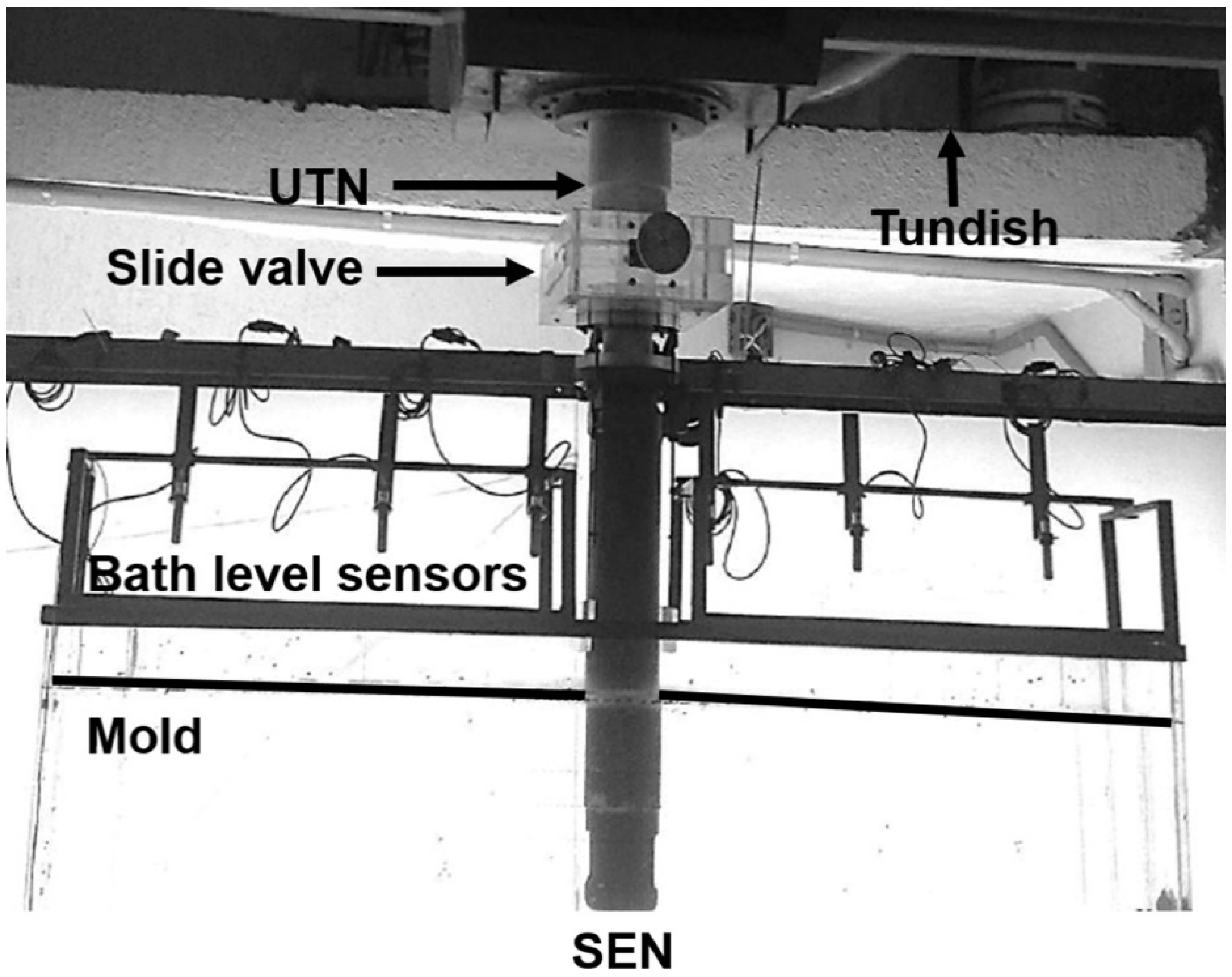
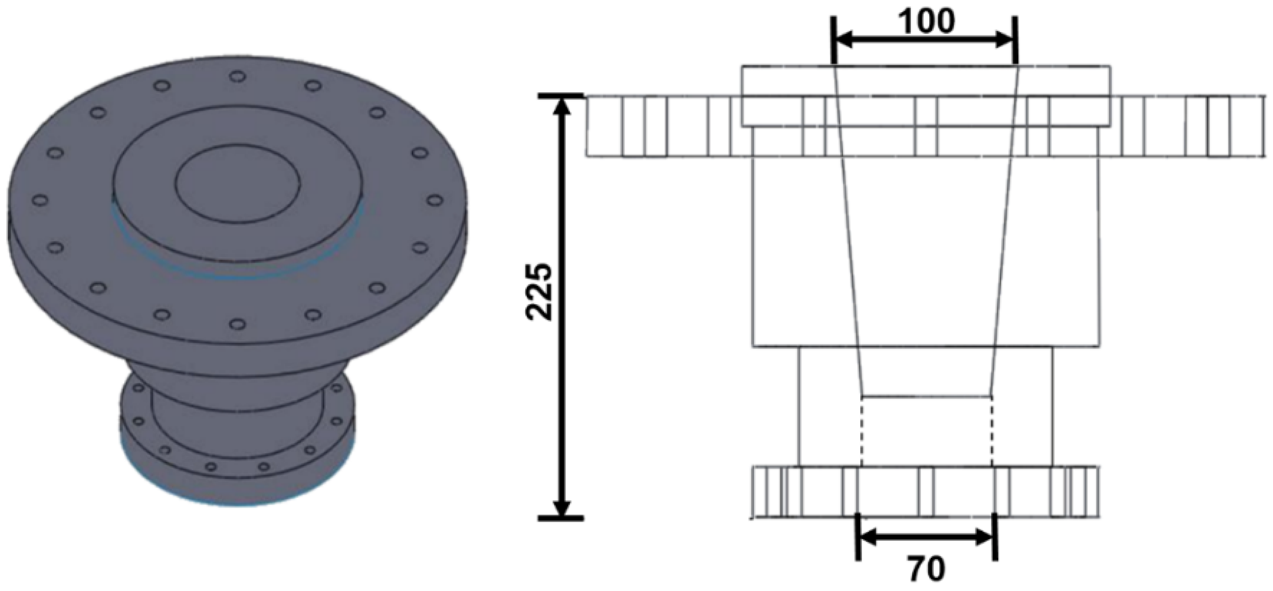
2. Experimental Techniques

The experimental set up consists of a full-scale water model of a mold, respecting the Reynolds and Froude numbers of the actual slab mold, with dimensions of 1650 mm × 200 mm × 1700 mm (width-thickness-height), made with 16 mm thick, transparent plastic sheets. This plastic mold is embedded 200 mm in an 1800 mm depth water tank, leaving a distance of 1500 mm outside the tank, ready to visualize the water’s flows. The joint perimeter between the mold and the tank is sealed with rubber rings and plastic foam to avoid water leaks. A water pump, immersed in the tank, pumps water to a tundish located above the mold. In the pipe that transports the water from the tank to the tundish (with a water column of 1 m, same as in the industrial tundish), there is a mass flowmeter and two valves to control it throughput required to fix the desired casting speed. The water’s level in the mold (meniscus) is 100 mm below the mold’s top. During an experiment, the water’s instantaneous level variations are continuously measured and recorded by six ultrasonic level sensors (Carlo Gavazzi, Milan, Italy) located 120 mm above the static level of the water in the mold. The ultrasonic analogic signals generated by these sensors are captured and processed to obtain digital signals through a data acquisition card, and these data are stored in a computer. Three sensors are on the nozzle’s right side, and three on the left side in fixed positions to detect the meniscus’ standing waves. This arrangement permits the plotting of the liquid’s instantaneous level variations during the performance of an experiment. Figure 1 shows a photo of the experimental mold.

The recording of the liquid’s flow patterns in the mold is through the technology of particle image velocimetry (PIV, DANTEC Systems, Conpenhaguen Dnmark ). The laser sheet passes through the center plane at the meniscus level; details of this technology are available in references [18,19]. The SV of the model consists of a faithful replica of the current one made of three overlapped plastic plates with central orifices. An endless screw, attached to the middle plate, works to increase or decrease the off-centering of the orifices to fix the water throughput. Figure 2a shows the full ensemble, including the upper tube nozzle (UTN), the valve, and the nozzle, manufacturing 3D prints and ensambling them in a machined plastic pipe. The model nozzle consists of a machined plastic tube and a 3D printed tip glued to the tube; Figure 2b shows the plastic nozzle’s characteristics and dimensions. Figure 3 shows the UTN’s geometric dimensions to the tundish bottom and connecting it with the nozzle. The casting speeds of this plant are 0.9 m/min, 1.3 m/min, and 1.65 m/min, the corresponding water flow rates, corrected by the solidification of the steel and the physical properties of liquid steel (solid steel density is 7800 kg·m⁻³) and water, are reported in

Table 2. Experimental conditions and physical properties.

Parameter		Value
Casting speed (m/min)		0.9, 1.3 and 1.65
Casting speed (m/s)		0.015, 0.0216667 and 0.0275
Water flow rate (L/s)		5.41, 7.81 and 9.92
Physical properties of water (20 °C)
Density (kg/m3)	Kinematic viscosity (m2/s)		Surface tension (N/m)
1000	1 × 10−6		0.073
Physical properties of liquid steel (1550 °C)
Density (kg/m3)	Kinematic viscosity (m2/s)		Surface tension (N/m)
7014	0.913 × 10−6		1.6

. The tundish is mounted in a frame with 3D motions, making it possible to test different nozzle immersions. The start of an experiment consisted of running the liquid for 20–25 min to reach steady-state conditions. After this period, the PIV system started to work, and the level sensors began the capture of data, as explained above.

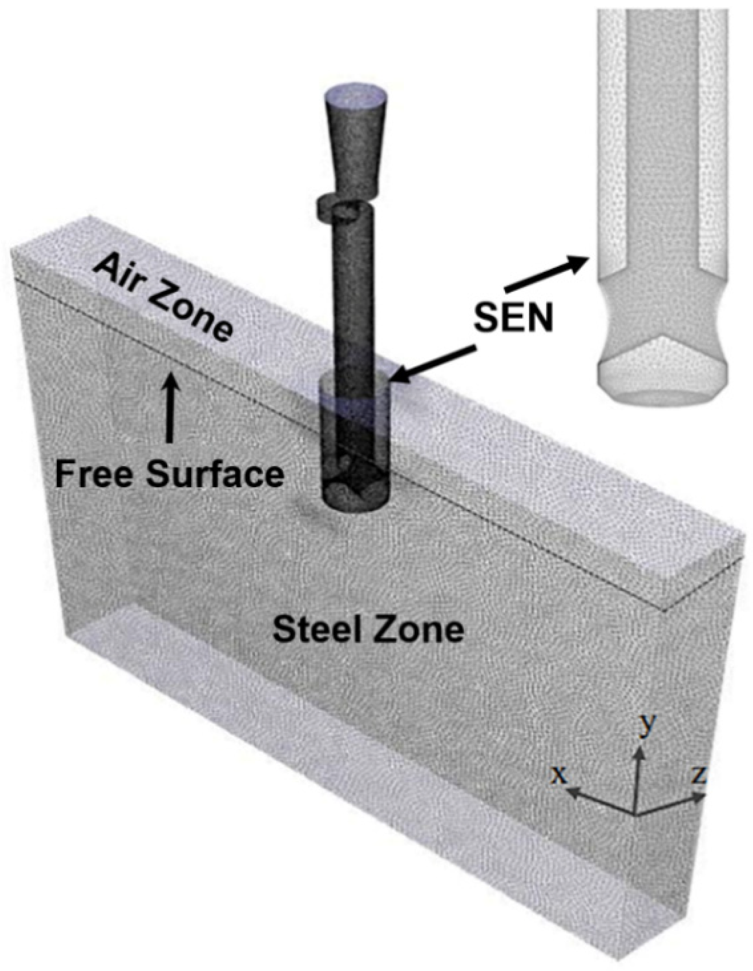
3. The Mathematical Model

The mathematical model consists of the simultaneous numerical solution of the Navier–Stokes and continuity equations using three different models. First, the k-ε, Reynolds-averaged Navier–Stokes (RANS) model simulates the first 300 s of real casting time, and then the numerical approach is switched to the large eddy simulation (LES) model for the other 300 s, using the results of the k-ε model as an initial condition. This approach is very convenient as the numerical simulations by the k-ε model supply averaged fluid velocities, which are discernible when explaining the flow patterns’ details. On the other hand, the LES model gives insight into actual instantaneous velocities in the field. Moreover, using k-ε results as the initial condition helps to reach faster convergence of the LES model. The volume of fluid model (VOF) works to solve the motion equations to unveil the liquid meniscus’ topography dynamics. Both models are summarized in the next lines.

3.1. The Mathematical Models

The basis of the k-ε and VOF models is the simultaneous solution of one set of turbulent continuity and momentum transfer expressed in tensorial form as,

$$\frac{\partial }{\partial x}\left(\rho \langle U_i\rangle \right)=0$$

(1)

$$\frac{\partial }{\partial t}\left(\rho \langle U_i\rangle \right)+\frac{\partial }{\partial x_j}\left(\rho \langle U_i\rangle \langle U_j\rangle \right)=-\frac{\partial \langle p\rangle }{\partial x_i}+\frac{\partial }{\partial x_j}\left[{\mu }_t\left(\frac{\partial \langle U_i\rangle }{\partial x_j}+\frac{\partial \langle U_j\rangle }{\partial x_i}-\frac{2}{3}{\delta }_{ij}\frac{\partial \langle U_i\rangle }{\partial x_j}\right)+\frac{\partial }{\partial x_j}\left(-\rho \overline{u_i{u}_j}\right)\right]+\rho g+F$$

(2)

In the conception of these equations, it is implicit the Reynolds decomposition $U_i\langle =\langle U_i\rangle +u_i$. Thus, these equations describe the mass and momentum balances through averaged velocities and pressure. For this reason, these models receive the name of the Reynolds-averaged Navier–Stokes or RANS models. The term $\rho \overline{u_i{u}_j}$ represents other six additional unknowns and having only four equations (continuity and three for momentum), there is a deficit of 6 equations to close the system. The RANS models avoid the solution of other six equations through a relation linking the Reynolds stresses with a turbulent viscosity provided through the Boussinesq’s relationship [20,21]:

$$-\rho \langle u_i{u}_j\rangle +\frac{2}{3}\rho k{\delta }_{ij}=\rho {\nu }_t\left(\frac{\partial \langle U_i\rangle }{\partial x_j}+\frac{\partial \langle U_j\rangle }{\partial x_i}\right)=2\rho {\nu }_t{\overline{S}}_{ij}$$

(3)

The central axis of the model is the estimation of the turbulent kinetic energy through,

$${\nu }_t=C_{\mu }\frac{k^2}{\epsilon }$$

(4)

where k is the turbulent kinetic energy given by half the tracer of the Reynolds stresses tensor,

$$k=\frac{1}{2}\langle u_i{u}_i\rangle$$

(5)

Though the turbulent viscosity is a fifth unknown, the system is maintained through the additional equation given in Equation (4) using two additional unknowns, the turbulent kinetic energy and its disipation rate solved through other two equations. Hence, there are 7 unknowns (pressure, three velocities, turbulent viscosity, the kinetic energy, and its dissipation rate) and seven equations.

According to Equation (4), two additional balances for the kinetic energy and its dissipation rate, are necessary, in order to calculate the turbulent viscosity and making possible the link between the Reynolds stresses and the mean deformation rate of the fluid element, i.e., Equation (3):

• Kinetic energy

  $$\frac{\partial k}{\partial t}+\langle U_j\rangle \frac{\partial k}{\partial x_j}={\tau }_{ij}\frac{\partial \langle U_i\rangle }{\partial x_j}-\epsilon +\frac{\partial }{\partial x_j}\left[\left(\nu +\frac{{\nu }_t}{{\sigma }_k}\right)\frac{\partial k}{\partial x_j}\right]$$

  (6)
• Dissipation rate of kinetic energy

  $$\frac{\partial \epsilon }{\partial t}+\langle U_j\rangle \frac{\partial e}{\partial x_j}=C_{\epsilon 1}\frac{\epsilon }{k}{\tau }_{ij}\frac{\partial \langle U_i\rangle }{\partial x_j}-C{\epsilon }_2\frac{{\epsilon }^2}{k}+\frac{\partial }{\partial x_j}\left[\left(\nu +\frac{{\nu }_t}{{\sigma }_{\epsilon }}\right)\right]$$

  (7)

The closure constant are, C_ε1 = 1.44, C_ε2 = 1.92, C_μ = 0.09, σ_k = 1.0, σ_ε = 1.3. These equations must be solved together with the averaged velocity continuity and Navier–Stokes equations using appropriate numerical schemes.

The volume of fluid (VOF, another RANS model) [22,23], employs only one set of continuity and momentum transfer equations for both phases (including balances for the kinetic energy and the dissipation rate of kinetic energy), water and air. The last term F, in Equation (2), is the force source related to the interface tension between air and water according to [24],

$$F={\sigma }_{ij}\frac{\rho {\kappa }_i\nabla {\alpha }_i}{\frac{1}{2}\left({\rho }_i+{\rho }_j\right)}$$

(8)

The expressions for the system’s physical properties, density, and viscosity, correspond to a simple mixture weighted by the volume fractions. Accordingly, we have $\rho =\sum {\rho }_q{\alpha }_q$, $\mu =\sum {\mu }_q{\alpha }_q$. Regarding the volume fractions, there is one Equation for the n − 1 phases providing the unknown volume fractions. The restriction of volume fractions is ${\sum }_1^n{\alpha }_q=1$, then the volume fraction of the last phase is ${\alpha }_n=1-{\sum }_1^n{\alpha }_q$. The differential equations of the volume fractions are:

$$\frac{\partial {\alpha }_q}{\partial t}+\left(\langle U\rangle ·\nabla \right){\alpha }_q=0$$

(9)

The solution procedure implies calculating the volume fraction, ${\alpha }_q$, which represents the cell’s fractional volume occupied by the fluid q and varies from zero to one. The tracking of the water-air interface is through solving the system of Equation (9) using an explicit scheme setting a Courant number of 0.5:

$$\frac{{\alpha }_q^{n+1}{\rho }_q^{n+1}+{\alpha }_q^n{\rho }_q^n}{∆t}+{\displaystyle \sum }_f\left({\rho }_q^n\left(\langle U^n\rangle \right){\alpha }_{q,f}^n\right)=0$$

(10)

where n + 1 is the unknown at present and n is at the previous one, ${\alpha }_q$ is the volume fraction of the primary phase q (water in the present case), and the surface area, and f stand for all faces of the finite volume. More details of the model are in references [22,23].

3.2. The LES Model

This model divides the spectrum of energy in two parts, the first involves the large scales and embodies the largest energies energies and the second is related with dissipation of energy at small scales [25,26]. The first part is simulated and the second is modeled. To proceed with this model, the Navier–Stokes equations are filtered, for example, the filtered velocity is,

$$\overline{U}\left(x,t\right)={\displaystyle \int }G\left(r,x\right)U\left(x-r\right)dr$$

(11)

where the integration is over the entire flow domain, and the specified filter function G sattisfy the normalization condition,

$$G\left(x,r\right)={\displaystyle \int }G\left(x,r\right)dr=1$$

(12)

The model generates a residual field defined as

$$u^{\prime }\left(x,t\right)=U\left(x,t\right)-\overline{U}\left(x,t\right)$$

(13)

So that the velocity field has the decomposition

$$U\left(x,t\right)=\overline{U}\left(x,t\right)+u^{\prime }\left(x,t\right)$$

The filtration of the Navier–Stokes equations yields,

$$\frac{\partial {\overline{U}}_i}{\partial x_j}=0$$

(14)

$$\frac{\overline{D}{\overline{U}}_j}{\overline{D}t}=\nu \frac{{\partial }^2{\overline{U}}_j}{\partial x_i\partial x_i}-\frac{1}{\rho }\frac{\partial \overline{p}}{\partial x_j}-\frac{\partial {\tau }_{ij}^r}{\partial x_i}+g$$

(15)

the term on the left side of Equation (15) is the operator, $\frac{\overline{D}( )}{\overline{D}t}=\frac{\partial ( )}{\partial t}+\overline{U}·\nabla ( )$. Moreover, i and j are tensor notation, repeated summation indicates a summation operation. ${\overline{U}}_i$ is the filtered three-velocity components, $\nu$ is the kinematic viscosity, $g$ is gravity constant, and ${\overline{p}}_i$ is the filtered pressure. The variable ${\tau }_{ij}^r$ is the residual stress term that involves all interactions between large and small eddies, and between small eddies themselves. To close the system’s equations, this stress tensor’s modeling is through the Smagorinsky–Lylli model [27].

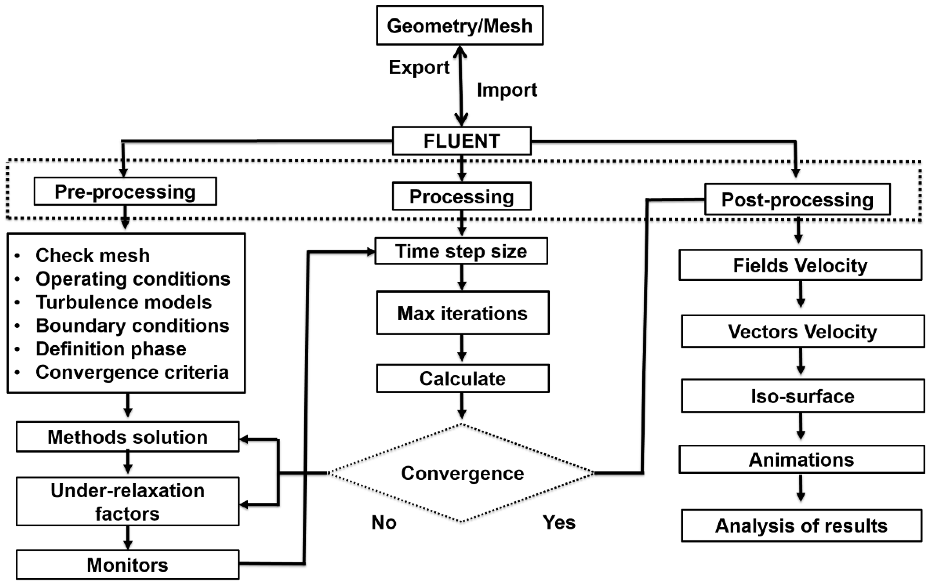
3.3. Numerical Schemes

The boundary conditions and the details of the computing procedure are reported in

Table 3. Computing features abd boundary conditions for the Reynolds-averaged Navier–Stokes (RANS), volume of fluid (VOF), and large eddy simulation (LES) models.

Concept	Implementation	Observations
Discretization of the computing mesh	Fisrst upwind shifted to second upwind	RANS model uses 1st upwid and LES model uses 2nd upwind
Iteration	Iterative Time Advancemnet
Mesh geometry	Tetraedral	1 853 907 cells
Input turbulence	Turbulence generator [28]	Generation of turbulent field in the input
Interpolation	Gradient method [29]
Pressure-velocity algorithm	SIMPLE [30] and PISO [31]	Simple for RANS-LES and PISO for VOF
Near wall velocities	Wall function and WALE	Wall function for RANS and VOF. WALE for LES [32]
Velocities in the walls	Velocities are zero
Fluid velocities at the inlet	Use liquid throghput	Throghputs calculated using the Bernoulli equation.
Pressure abiove the system	101 325 Pa
Convergence criterion	Sum of all residuals < 10−4	Time step 0.001−0.05 swith 500 hundred iterations as average

.

Figure 4 shows the computational mesh used to solve the equations and Figure 5 shows a generic flow diagram to explain the computing procedure to perform mathematical simulations. The full system of equations was solved through the ANSYS-FLUENT software [32].

4. Results and Discussion

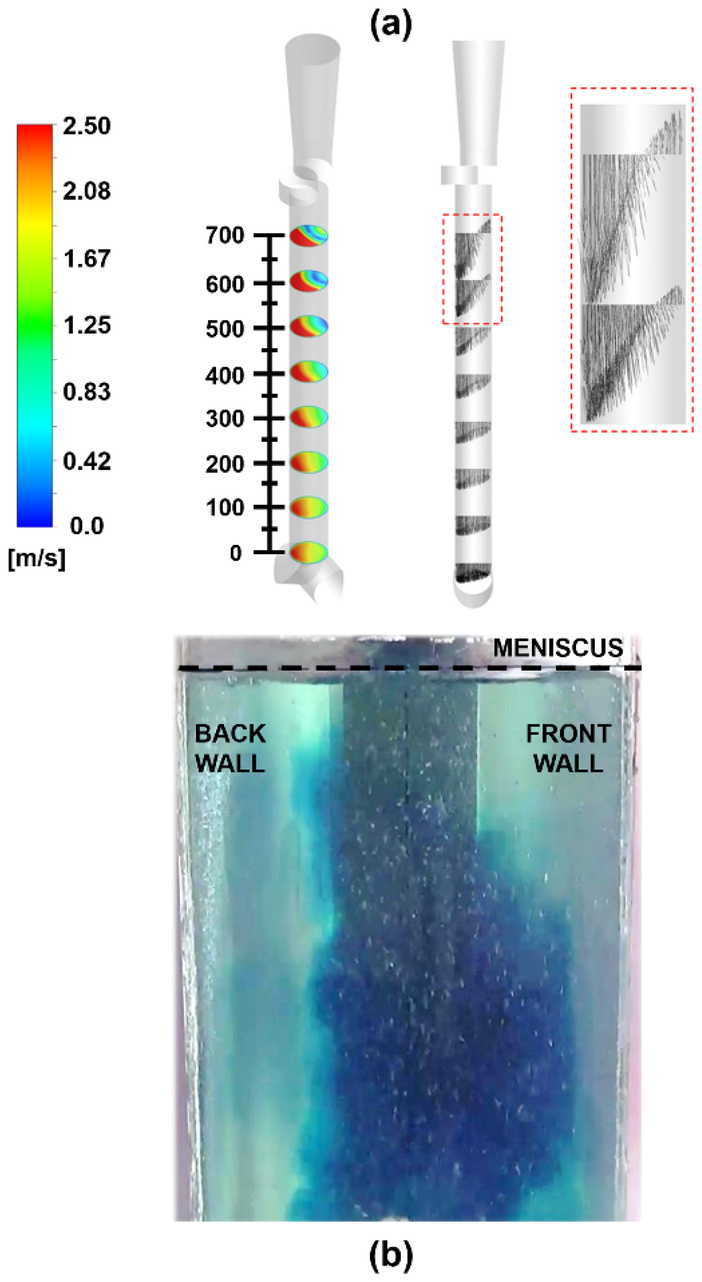
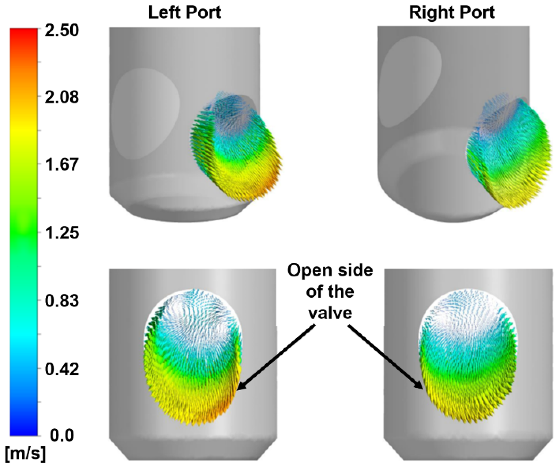
4.1. Fluid Flow through the Nozzle

Figure 6a shows the fluid flow through the nozzle; indeed, the highest velocities are in the valve opening side. Though heat transfer is not simulated in this work, it is evident that biased flows will bring heterogeneous heat fluxes through the copper plates of the mold. In the upper region, below the SV, there is counterflow due to recirculation. The biased flow condition remains until the end of the pipe, at the level of the two discharging ports. A blue dye tracer injected in the upper tube nozzle, Figure 6b, shows the biased flow-oriented to the frontal mold’s broad face, in the same orientation of the valve’s opening. This condition of biased velocity profiles inside the nozzle is transmitted to the discharging jets that generate asymmetrical flows in the mold. Figure 7a shows the velocity field calculated by the k-$\epsilon$ model with the typical double roll flow pattern formed after the jet’s impact with the narrow face. As seen in this figure, the port’s surface area utilized for the flow is small, and the largest velocities of the fluid are concentrated in its lower edge. Figure 7b provides the mathematical simulation validation through the water’s velocity profile in a plane perpendicular to the sheet, close to the port (line 1 in the figure), determined by the PIV. The peak velocity is close to 1.5 m/s, and it is at a level of about 20 mm from the level of the lower edge of the port, decreasing to 0.2 m/s at a level of 60 mm from the same reference. These numerical and experimental results agree in the characteristic of poor utilization of the port for the fluid flow. Downstream, the jet flow inline 2, on the same right side of Figure 7b, the velocity profile flattens considerably, having a minimum that is well predicted by the mathematical model, and indicated by the red arrows in Figure 7a.

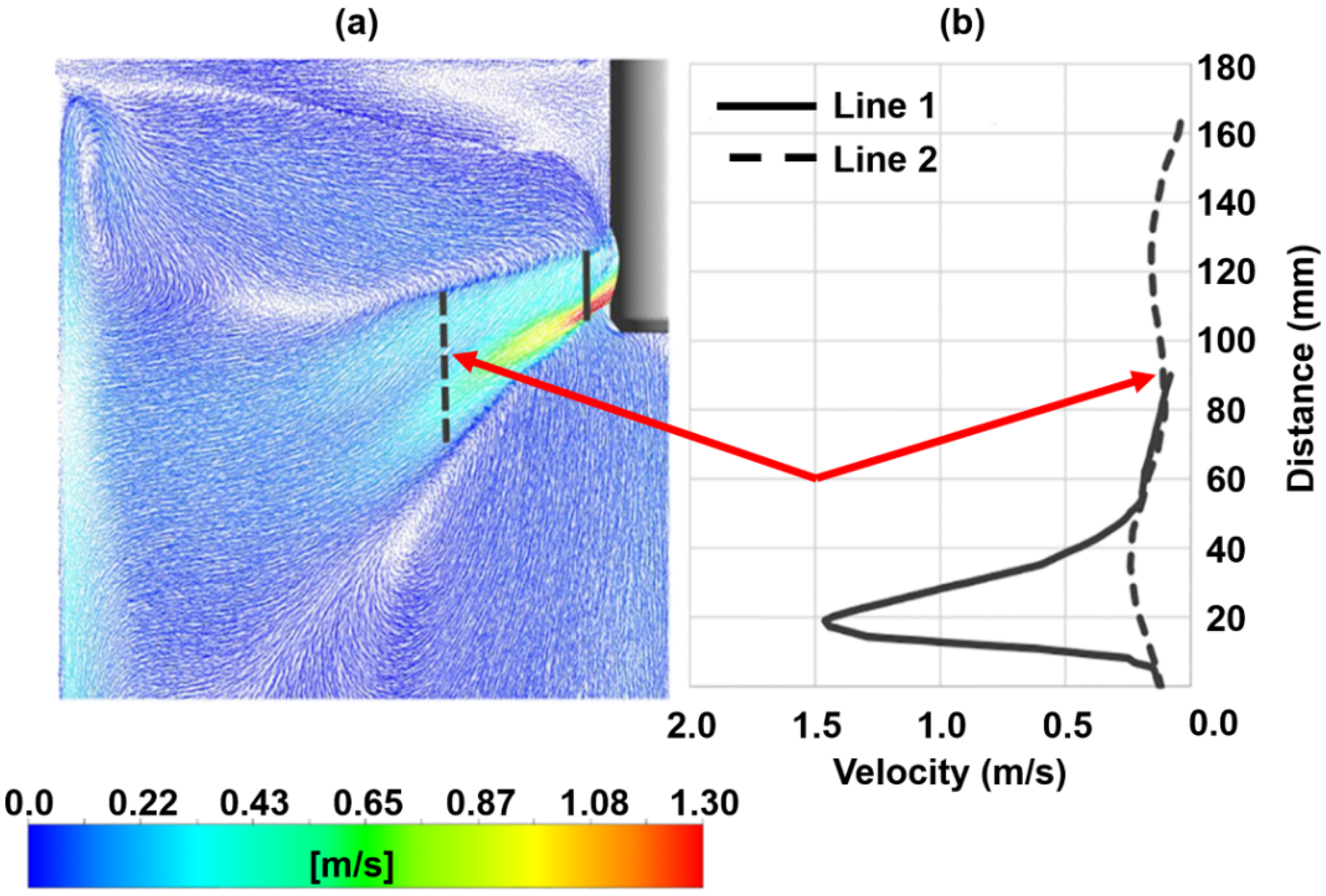
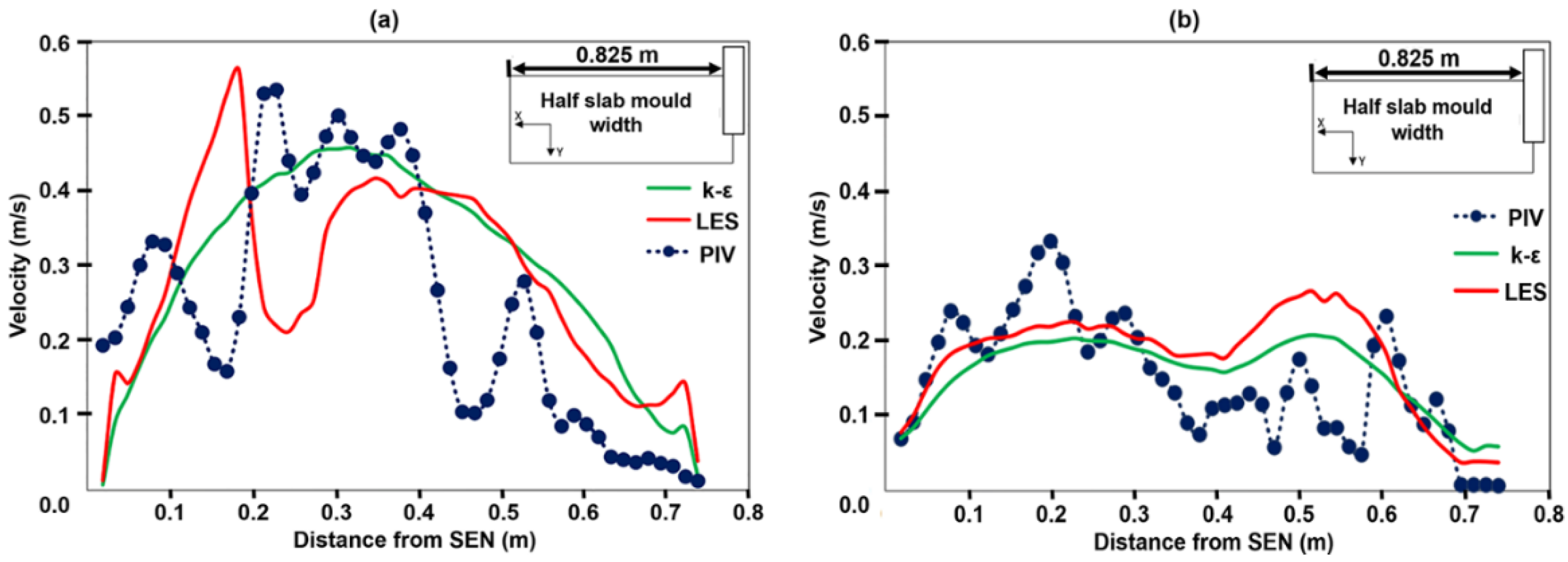
4.2. Velocity Fields by Mathematical Modeling

The casting speed and the nozzle immersion (measured from the top edge of the port to the meniscus level) change the flow patterns radically in the mold. Figure 8a–c show the LES model’s velocity fields in the central plane and the back and frontal planes, respectively, for a casting speed ($V_c$) of 1.3 m/min and a nozzle immersion of 95 mm. The velocities in the meniscus’ proximities are small compared to the lower roll flow velocities, forming, essentially, a single roll flow. Figure 8a shows the asymmetry of the flow under these operating conditions.

Figure 9a–c show the same planes corresponding to the velocity fields of Figure 8a–c, and the same casting speed with a nozzle immersion of 185 mm. Now, the meniscus’ fluid velocities are larger than in the previous case, and this flow follows a double roll flow pattern. The velocity fields in horizontal planes close to the meniscus are reported in Figure 10a,b, for a nozzle immersion of 95 mm at casting speeds of 0.9 m/min and 1.3 m/min; and Figure 10c,d for a nozzle immersion of 185 mm at the same casting speeds. Looking at these figures, it is evident that casting with a speed of 0.9 m/min and a nozzle immersion of 185 mm represents the worst scenario, due to the small velocities near the meniscus.

Under these conditions, there will be thick shells at the meniscus level, resulting in longitudinal cracking and early solidification in the whole meniscus region. The consequences of the flows shown in Figure 8, Figure 9 and Figure 10 on the slab quality are summarized in

Table 4. Effects of flow patterns in the mold on the final steel product.

Casting Speed (m/min)	Nozzle Immersion (mm)	Effects on Quality of Steel Sheets
0.9	95	A single flow roll causes flux entrainment particles, which become inclusions in steel sheets. However, it can keep a hot meniscus to melt the flux and forming thin shells.
1.3	95	This condition yields a single roll flow pattern. Higher liquid velocities cause flux entrainment, forming exogeneous inclusions in the final steel sheet.
0.9	185	The discharging jets barely impact the mold´s narrow faces leaving a stagnant meniscus. This condition will lead to excessive shell thicknesses deriving of longitudinal cracks.
1.3	185	Flow maintains a hotter steel due to the larger fluid velocities in the meniscus. Rapid melting of the mold flux. The probability for the formation of hook cracks decreases.

Therefore, the simple immersion of the nozzle and the biased flow may significantly affect the final product’s quality. Figure 11 shows the velocity profiles in the left and right nozzle’s ports, for a casting speed of 1.3 m/min and a nozzle immersion of 185 mm. The arrows indicate the valve opening’s orientation, characterized by the largest velocities observed in the valve opening side. The flow’s asymmetry is evident by the still larger velocities observed in the left port than in the right one.

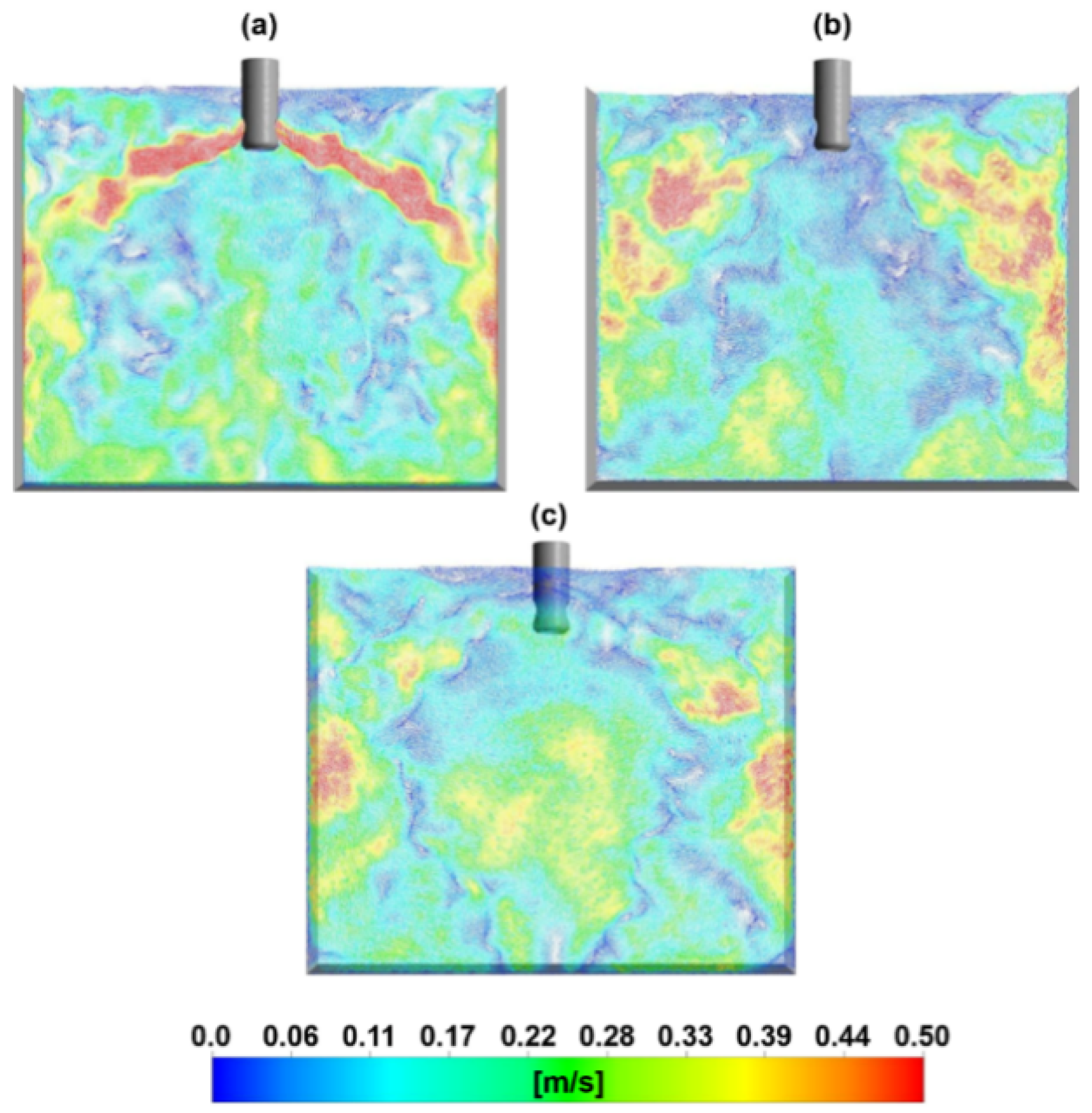
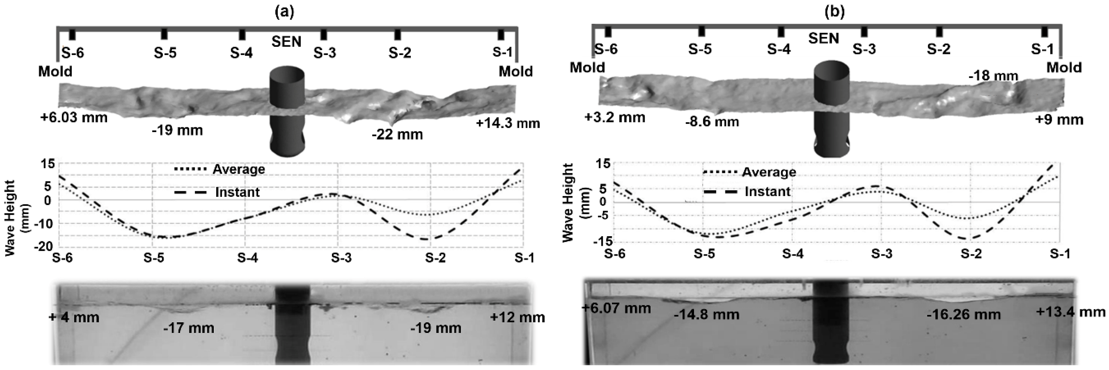
4.3. Meniscus Topography

Maintaining a fixed casting speed at 1.3 m/min and varying the nozzle immersion changes the topography of the bath surface, due to different amplitudes of the standing wave, as seen in Figure 12a,b, corresponding to immersions of 95 mm and 185 mm, respectively. The bath surface topography, simulated through the VOF model, is wavier in the second case, which yields a larger wave amplitude. The bath surface depressions predicted by the model match those observed in the photos and the experimental measurements with the ultrasonic sensors. These results agree with the type of flow, single, and double roll, presented in Figure 12a,b, respectively. In the first case, the jet delivers the liquid directly to impact the narrow faces, generating a downstream flow toward the mold’s lower region. In the second case, the jet, after impacting the narrow face, forms an upper flow coming back toward the nozzle, and another flow coming down along that face.

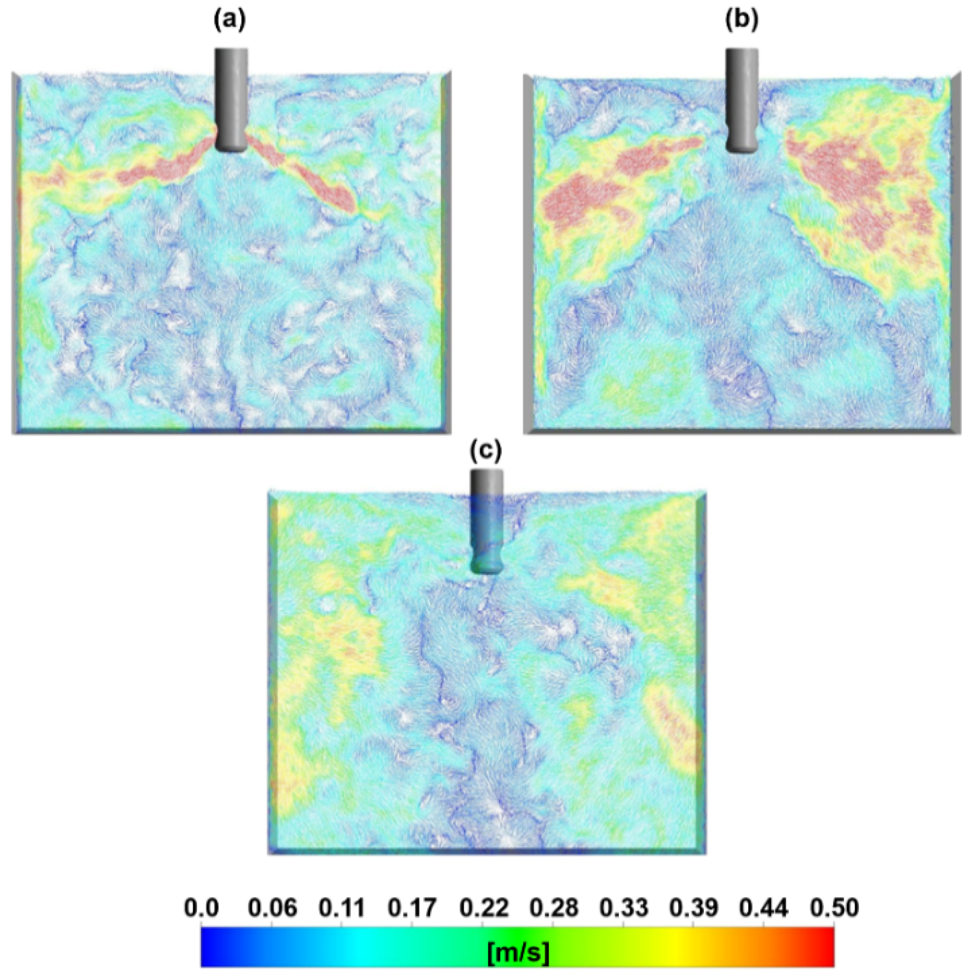
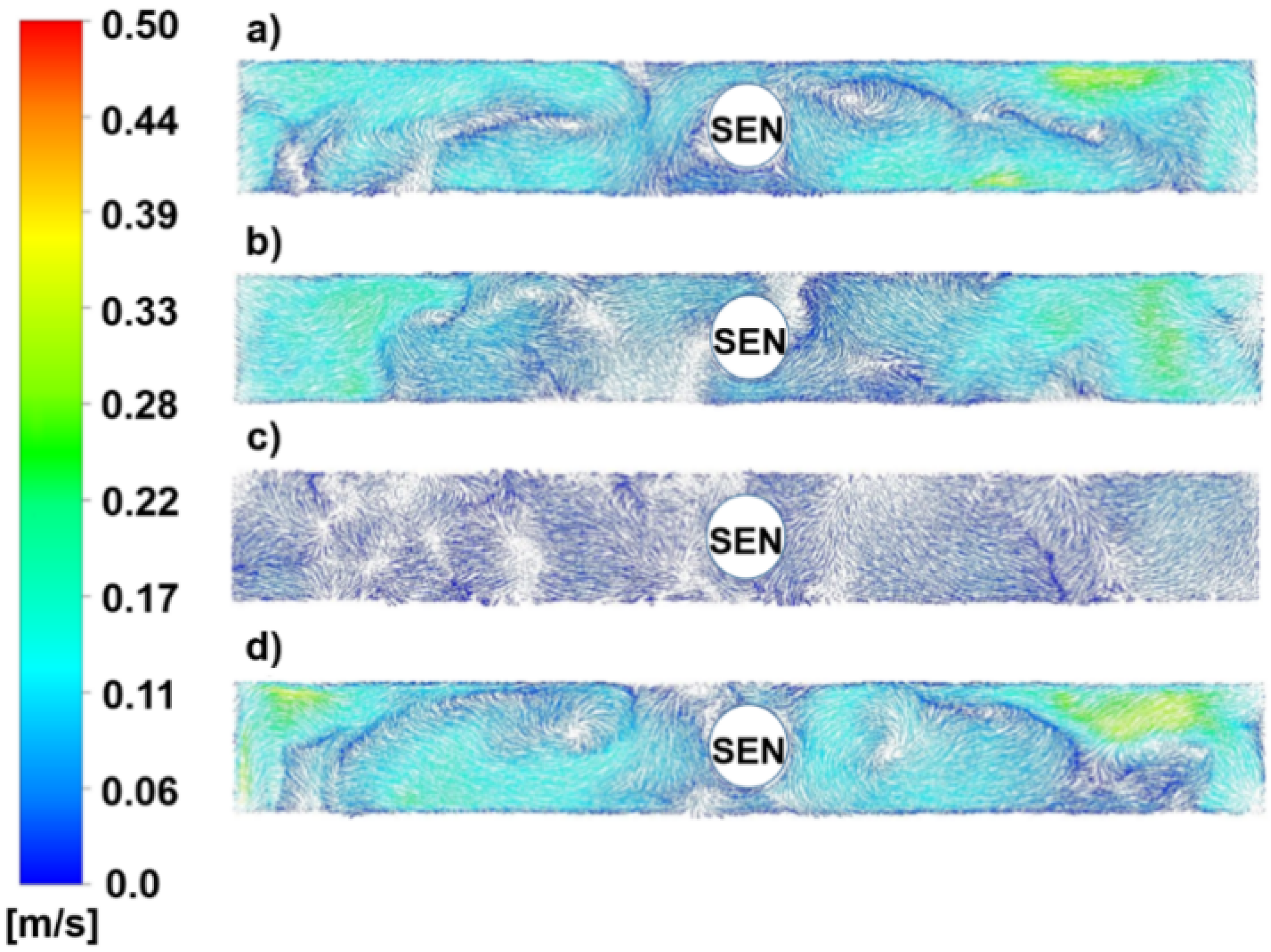
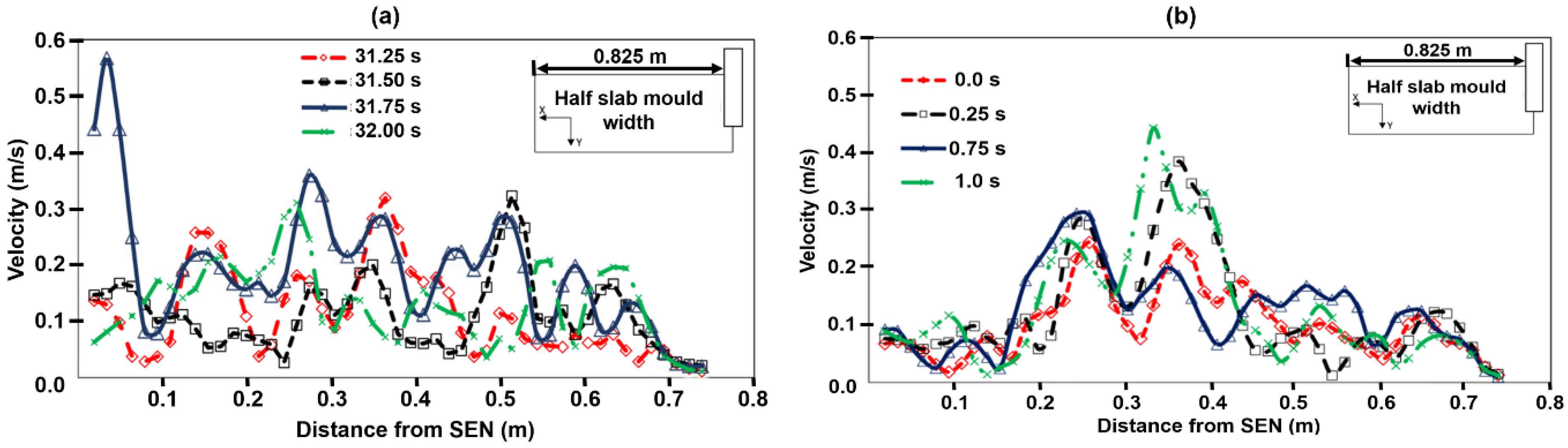
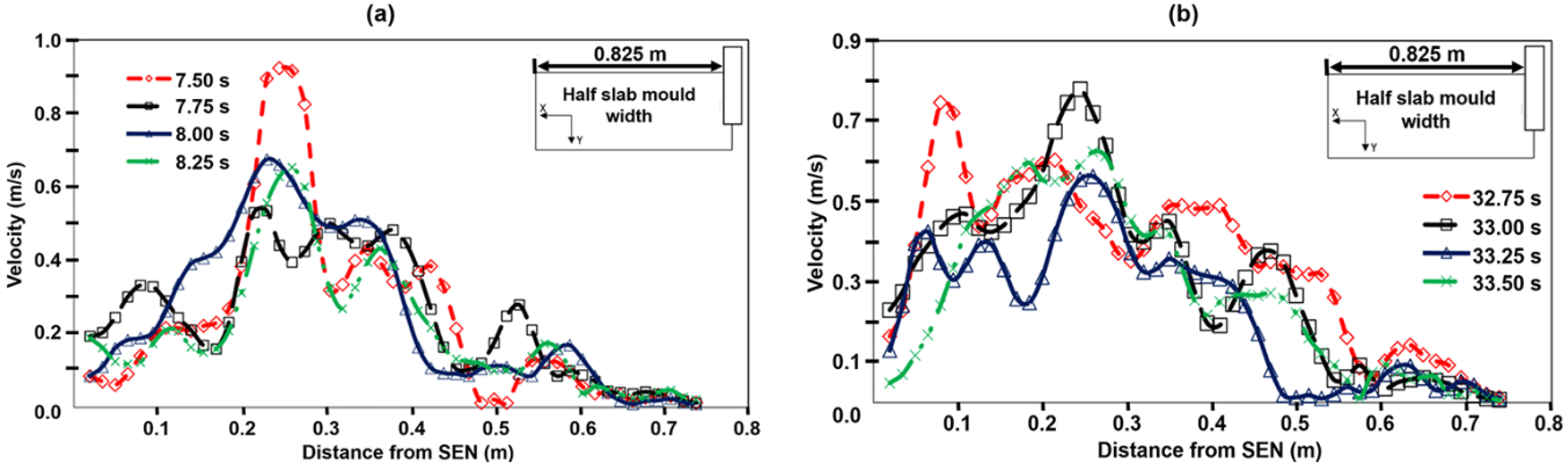
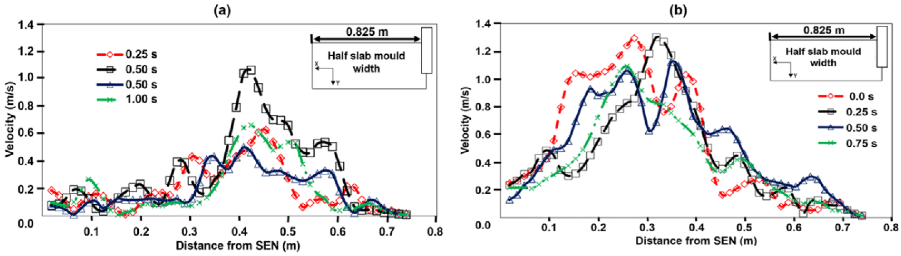
4.4. Dynamics of Sub-Meniscus Velocities

Figure 13a,b show the fluid’s transient velocity profiles along with the meniscus, measured by PIV techniques, from the narrow wall to the nozzle position at time intervals of 0.25 s, for a casting speed of 0.9 m/min at immersions of 95 mm and 185 mm, respectively. At the shallow immersion, for one second, a large variability of velocity is observed, along with this distance with multiple velocity peaks. This effect is indicative of an ill-defined wave, or probably a series of waves on the bath surface, due to the generation of a single flow roll pattern. Therefore, the momentum transfer is practically oriented from the nozzle toward the narrow wall. At the deeper position, a well-defined region of peak velocities is observed between 0.3 m and 0.45 m, which is indicative of the existence of a large amplitude-wave under this condition. It is essential to notice that velocities’ variability at the deep position decreases, although the peak velocity reaches a magnitude close to 0.45 m/s.

Figure 14a,b show the corresponding plots at a casting speed of 1.3 m/min; the peak velocities are now between 0.2–0.3 m from the narrow wall, variability with time, close to the nozzle the velocities remain small. Figure 14a corresponds to the shallow immersion. At the deep position, bimodal velocity profiles are generated with a new peak velocity close to the narrow face, Figure 14b. The region in the first 0.1 m from the narrow face observes the highest velocities.

Figure 15a,b show the velocity profiles for a casting speed of 1.65 m/min; at the shallow position, the velocity peak is at a distance 0.35–0.5 m from the narrow face. Variations with time remain relatively small in the mold corner and close to the nozzle. At the nozzle’s deep position, the velocity peak is now displaced to the narrow face, but the wave features have a more extended width. Some peak velocities exceed 1 m/min. These effects are summarized as follows here:

• At shallow immersions and low casting speeds, the flow behaves essentially as a single roll flow. The flow changes to a partial double roll flow at deep immersions.
• Increasing the casting speed at shallow immersions displaces the region of velocity peaks toward the nozzle, and deep immersions displace this region toward the narrow wall.
• The region yielding high-velocity peaks gets wider with deep immersions, and the region close to the nozzle remains quite for any case.
• The region close to the narrow wall observes high turbulence levels with deep immersions and high casting speeds.

Figure 16a,b show instantaneous velocity profiles determined through PIV, and simulation results using the k-ε and LES models, for a casting speed of 1.3 m/min at immersions of 95 and 185 mm, respectively. The shallow position yields, in general, higher meniscus velocities than the deep one. The first observation is that there is no perfect matching between PIV measurements and the two simulated profiles, due to the impossibility to match the three times, the experimental time, and computational times of k-ε and LES models. However, as seen, predictions using the three approaches follow the same general trend. For example, both simulations predict a double velocity peak flow, such as Figure 16b and PIV measurements; even though yield a more irregular profile, it keeps the same double peak tendency.

Moreover, there is an agreement of a single velocity peak between PIV measurements and predictions made by the k-ε model, Figure 16a. Predictions by the LES model are now more irregular, but the general trend is maintained again. The important observation here is that predictions using either of the two models show the PIV measurements’ general trend. It is also clear that the k-ε model predicts time-averaged velocities, and the instantaneous changes of velocity can only be visualized through LES. In conclusion, LES is recommendable to follow, mathematically, the dynamic behavior of the meniscus velocities.

5. Casting Diagnosis

The length of the zirconia belt to protect the nozzle from the flux attack has a length of 100 mm, and the caster tries to harness the use of its total length to prolong the casting sequence. This condition drives the decision to use a shallow immersion like 95 mm and a depth immersion as large as 185 mm. However, at either low or high casting speeds, the shallow immersion yields single roll flow patterns producing defects on the product as reported in Table 4. At very high casting speeds (1.3–1.65 m/min), the liquid velocities reach magnitudes of 1–1.2 m/min at shallow or deep immersions. Such velocities result in abundant flux entrainment affecting the level of steel cleanliness [33]. Due to the nature of the SV, biased flows are always present. The extent of the biased flow is still considerable at a casting speed of 1.3 m/min, as evidenced by the tracer in Figure 6b.

6. Recommendations

The current nozzle has a limited window of acceptable mold operating conditions, which include casting speeds higher than 0.9 m/min and deeper immersions than 95 mm. However, these casting conditions (increasing immersion and casting speed) will serve as a palliative and not as a solution. Therefore, there is an evident need to redesign the nozzle to aim at two goals: lower liquid velocities in the meniscus at high casting speeds and the generation of symmetric flows. The key to attain those goals is the use of internal deflectors in the new nozzle, which have proven effective in other casters. However, these internal deflectors’ sizes and positions are crucial to obtain optimum casting products [34,35]. This new task involves extensive computer runs and the outputs will generate materials for further publications. The company has awarded the author’s laboratory the modification of the current nozzle.

7. Conclusions

Casting diagnosis of a mold operating with a bifurcated nozzle and a slide valve is carried out using experimental and mathematical tools. The conclusions derived from the results and their discussion are the following:

• The use of a slide valve inherently delivers biased flows through the bifurcated ports of a nozzle.
• A shallow nozzle immersion, such as 95 mm, is not recommended, as this condition induces a single roll flow pattern that has a propensity to drag flux in the metal bulk.
• Casting speeds like 1.65 m/min raise the liquid velocity at the meniscus level to magnitudes as high as 1.1–1.3 m/min. These velocities will drag flux in the metal bulk.
• This caster’s operating conditions demand a nozzle with a different design that must guarantee unbiased flows and stabilize the meniscus.
• The application of the k-ε, VOF, and LES models, combined with experimental techniques for current operating casters, proved suitable for process diagnosis.

References

1. Stemple, D.K.; Zulueta, E.N.; Flemings, M.C. Effect of Wave Motion on Chill Casting Surfaces. Metall. Mater. Trans. B 1982, 13, 503–509. [Google Scholar] [CrossRef]
2. Segupta, J.; Shin, H.-J.; Thomas, B.G.; Kim, S.-H. Micrograph evidence of meniscus solidification and sub-surface microstructure evolution in continuous-cast ultralow-carbon steels. Acta Mater. 2006, 54, 1165–1173. [Google Scholar] [CrossRef]
3. Bradi, A.; Natarajan, T.T.; Snyder, C.C.; Powders, K.D.; Mannion, F.J.; Byrne, M.; Cramb, A.W. Mold Simulator for Continuous Casting of Steel: Part II.The Formation of Oscillation Marks during the ContinuousCasting of Low Carbon Steel. Metall. Mater. Trans. B 2005, 36, 373–383. [Google Scholar]
4. Knoepke, J.; Hubbard, M.; Kelly, J.; Kittridge, R.; Lucas, J. Pencil blister reduction at inland steel company. In Proceedings of the 77th Steelmaking Conference, Iron and Steel Society, Chicago, IL, USA, 20–23 March 1994; pp. 381–388. [Google Scholar]
5. Emling, W.H.; Waugaman, T.A.; Feldbauer, S.L.; Cramb, A.W. Subsurface mold slag entrainment in ultra-low carbon steels. In Proceedings of the 77th Steelmaking Conference, Iron and Steel Society, Chicago, IL, USA, 20–23 March 1994; pp. 371–379. [Google Scholar]
6. Bai, H.; Thomas, B.G. Turbulent flow of liquid steel and argon bubbles in slide-gate tundish nozzles: Part I. Model development and validation. Metall. Mater. Trans. B 2001, 32, 253–267. [Google Scholar] [CrossRef]
7. Bai, H.; Thomas, B.G. Turbulent flow of liquid steel and argon bubbles in slide-gate tundish nozzles: Part II. Effect of operation conditions and nozzle design. Metall. Mater. Trans. B 2001, 32, 269–284. [Google Scholar] [CrossRef]
8. Thomas, B.G. Modeling of continuous casting. In Proceedings of the 3rd International Congress on Science and Technology of Steelmaking, AISTech, Charlotte, NC, USA, 9–12 May 2005; pp. 847–861. [Google Scholar]
9. Liu, Z.; Li, B.; Jiang, M. Transient asymmetric flow and bubble transport inside a slab continuous-casting mold. Metall. Mater. Trans. B 2014, 45, 675–697. [Google Scholar] [CrossRef]
10. Takatani, K. Effects of electromagnetic brake and meniscus electromagnetic stirrer on transient molten steel flow at meniscus in a continuous casting mold. ISIJ Int. 2003, 43, 915–922. [Google Scholar] [CrossRef]
11. Liu, R.; Sengupta, J.; Crosbie, D.; Yavuz, M.M.; Thomas, B.G. Effects of stopper rod movement on mold fluid flow at Arcelor Mittal Dofasco’s No. 1 continuous caster. In Proceedings of the Iron and Steel Technology Conference and Exposition, AISTech, Indianapolis, IN, USA, 2–5 May 2011; pp. 1–13. [Google Scholar]
12. Greis, B.; Bahrmann, R.; Ruckert, A.; Pfeifer, H. Investigations of flow pattern in the SEN regarding different stopper rod geometries. Steel Res. Int. 2015, 86, 1469–1479. [Google Scholar] [CrossRef]
13. Otsuka, A.; Harada, K.; Haruyuki, O.; Tsuneoka, A. New slide gate system for flow control. In Proceedings of the Iron and Steel Technology Conference, AISTech, Nashville, TN, USA, 15–17 September 2004; pp. 985–991. [Google Scholar]
14. Heinrich, B.; Stopinc, A.G.; Hackl, G.; Marshall, U. Adavantages of optimised flow control from ladle to tundish. In Proceedings of the METEC and 2nd ESTAD, Dusseldorf, Germany, 15–19 June 2015. [Google Scholar]
15. Najjar, F.M.; Thomas, B.G.; Hershey, D.E. Numerical study of steady turbulent flow through bifurcated nozzle in continuous casting. Metall. Mater. Trans. B 1995, 26, 749–765. [Google Scholar] [CrossRef]
16. Mills, K.C.; Fox, A.B.; Thackray, R.P.; Li, Z. Continuos casting mould powder and castind process interaction: Why powders do not always wok as expected. In VII International Conference on Molten Slags Fluxes and Salts; The South African Institute of Mining and Metallurgy: Johannesburg, South Africa, 2004; pp. 713–722. [Google Scholar]
17. Mills, K.C.; Sridhar, S. Viscosities of ironmaking and steelmaking slags. Ironmak. Steelmak. 1999, 26, 262–268. [Google Scholar] [CrossRef]
18. Milanovic, I.M.; Hammad, K.J. PIV study of the near field region of a turbulent round jet. In Proceedings of the 3rd Joint US-European Fluids Engineering Summer Meeting and the 8th International Conference on Nanochannels, Microchannels and Mini-channels, ASME, Montreal, QC, Canada, 1–5 August 2010; pp. 1–9. [Google Scholar]
19. Morales, R.D.; Palafox-Ramos, J.; García-Demedices, L.; Sanchez-Perez, R. A DPIV study of liqud steel flow in a wide thin slab caster using four ports submerged entry nozzles. ISIJ Int. 2004, 44, 1384–1392. [Google Scholar] [CrossRef] [Green Version]
20. Wilcox, D.C. Turbulence Modeling for CFD; DCW Industries: La Cañada, CA, USA, 2000; pp. 103–104. [Google Scholar]
21. Tennekes, H.; Lumley, J.L. A First Course on Turbulence; The MIT Press: Cambridge/London, UK, 1972; pp. 27–30. [Google Scholar]
22. Hirt, C.W.; Nichols, B.D. Volume of fluid (VOF) method for the dynamics of free boundaries. Comp. Phys. 1981, 39, 201–225. [Google Scholar] [CrossRef]
23. Yeoh, G.H.; Tu, J. Computational Techniques for Multiphase Flows; Butterworth-Heinemann: Oxford, London, UK, 2010; p. 215. [Google Scholar]
24. Brackbill, J.U.; Kothe, D.B.; Zemach, C. A continuum method for modeling surface tension. Comp. Phys. 1992, 100, 335–354. [Google Scholar] [CrossRef]
25. Sagaut, P. Large Eddy Simulation for Incompressible Flows; Springer-Verlag: Berlin/Heidelberg, Germany, 2000; pp. 1–291. [Google Scholar]
26. Pope, S. Turbulent Flows; Cambridge University Press, Cambridge Press: London, UK, 2000; pp. 558–638. [Google Scholar]
27. Smagorinsky, J. General Circulation Experiments with the Primitive Equations. I the Basic Experiment. Month. Weather Rev. 1963, 91, 99–164. [Google Scholar] [CrossRef]
28. Smirnov, A.; Shi, S.; Celik, I. Random flow generation technique for large eddy simulations and particle-dynamics modeling. J. Fluids Eng. 2001, 123, 359–371. [Google Scholar] [CrossRef]
29. Ferziger, J.H.; Peric, M. Computational Methods for Fluid Dynamics; Springer: New York, NY, USA; Berlin, Germany, 2002; p. 72. [Google Scholar]
30. Chung, T.J. Computational Fluid Dynamics; Cambridge University Press: London, UK; New York, NY, USA, 2002; pp. 106–119. [Google Scholar]
31. Issa, R.I. Solution of the implicitly discretized fluid flow equations by operator-splitting. Comp. Phys. 1986, 62, 40–65. [Google Scholar] [CrossRef]
32. ANSYS, Inc. Available online: www.Ansys.com (accessed on 10 April 2019).
33. Calderón-Ramos, I.; Morales, R.D. Influence of turbulent flows in the nozzle on melt flow within a slab mold and stability of the metal-flux interface. Metall. Mater. Trans. B 2016, 47, 1866–1881. [Google Scholar] [CrossRef]
34. González-Solórzano, M.G.; Morales, R.D.; Gutiérrez, E.; Guarneros-Guarneros, J.; Chattopadhyay, K. Analysis of Fluid Flow of Liquid Steel through Clogged Nozzles: Thermodynamic Analysis and Flow Simulations. Steel Res. Int. 2020, 91. [Google Scholar] [CrossRef]
35. Cedillo, V.; Morales, R.D. Biased flows in slab molds induced by slide gates. Part I: Experimental measurements and flow simulation. Ironmak. Steelmak. 2018, 45, 204–214. [Google Scholar] [CrossRef]
Figure 1. Full scale water model with bath level snesors and the slide valve.
Crystals 10 01035 g001
Figure 2. (a) Complete set of upper tube nozzle (UTN), slide gate or valve and nozzle (submerged entry nozzle, SEN). (b) Nozzle geometry. Dimensions in mm.
Crystals 10 01035 g002
Figure 3. Geometry of the upper tube nozzle (UTN). Dimensions in mm.
Crystals 10 01035 g003
Figure 4. Computational mesh used in the mathematical simulations.
Crystals 10 01035 g004
Figure 5. Mathematical simulations computational flowsheet.
Crystals 10 01035 g005
Figure 6. Fluid flow inside the nozzle. (a) Velocity profile affected by the slide valve opening. (b) A blue dye tracer showing the biased flow of the liquid oriented toward the mold’s broad (frontal) face.
Crystals 10 01035 g006
Figure 7. Fluid flow in the mold. (a) Mathematical simulation of the discharging jet and the flow pattern generated. (b) Velocity profile along the diameter of the discharging port.
Crystals 10 01035 g007
Figure 8. Flow fields of velocity simulated through the large eddy simulation model (LES). (a) Central plane. (b) Back plane. (c) Front plane. V c = 1.3 m/s and nozzle depth 95 mm.
Crystals 10 01035 g008
Figure 9. Flow fields of velocity simulated through the large eddy simulation model (LES). (a) Central plane. (b) Back plane. (c) Front plane. Casting speed, V c = 1.3 m/s and nozzle depth 185 mm.
Crystals 10 01035 g009
Figure 10. Velocity fields at the meniscus simulated by the large eddy simulation model (LES): (a) Casting speed = 0.9 m/min, depth 95 mm, (b) V c = 1.3 m/min, depth 95 mm, (c) V c = 0.9 m/min, depth 185 mm, (d) V c = 1.3 m/min, depth 185 mm.
Crystals 10 01035 g010
Figure 11. Velocity fields through the left and right discharging ports, simulated by the k-ε model. V c = 1.3 m/min, nozzle depth: 185 mm.
Crystals 10 01035 g011
Figure 12. Meniscus topography simulated through the volume of fluid model and bath level measurements. (a) Casting velocity = 1.3 m/min, nozzle depth: 95 mm. (b) Casting velocity = 1.3 m/min, nozzle depth: 185 mm.
Crystals 10 01035 g012
Figure 13. Velocity profiles in the sub-meniscus region measured by the particle image velocimetry (PIV). (a) V c = 0.9 m/min, nozzle depth: 95 mm. (b) V c = 0.9 m/min, nozzle depth: 185 mm.
Crystals 10 01035 g013
Figure 14. Velocity profiles in the sub-meniscus region measured by the PIV. (a) Casting speed = 1.3 m/min, nozzle depth: 95 mm. (b) Casting speed = 1.3 m/min, nozzle depth: 185 mm.
Crystals 10 01035 g014
Figure 15. Velocity profiles in the sub-meniscus region measured by the PIV. (a) V c = 1.65 m/min, nozzle depth: 95 mm. (b) V c = 1.65 m/min, nozzle depth: 185 mm.
Crystals 10 01035 g015
Figure 16. (a) Comparison of measured, by the PIV, and calculated velocity magnitudes at the sub-meniscus region using the LES and k-ε models. (a) V c = 1.3 m/min, nozzle depth: 95 mm. (b) V c = 1.3 m/min, nozzle depth: 185 mm.
Crystals 10 01035 g016