Topological Equivalence of the Phase Diagrams of Molybdenum and Tungsten

Abstract

We demonstrate the topological equivalence of the phase diagrams of molybdenum (Mo) and tungsten (W), Group 6B partners in the periodic table. The phase digram of Mo to 800 GPa from our earlier work is now extended to 2000 GPa. The phase diagram of W to 2500 GPa is obtained using a comprehensive ab initio approach that includes (i) the calculation of the $T=0$ free energies (enthalpies) of different solid structures, (ii) the quantum molecular dynamics simulation of the melting curves of different solid structures, (iii) the derivation of the analytic form for the solid–solid phase transition boundary, and (iv) the simulations of the solidification of liquid W into the final solid states on both sides of the solid–solid phase transition boundary in order to confirm the corresponding analytic form. For both Mo and W, there are two solid structures confirmed to be present on their phase diagrams, the ambient body-centered cubic (bcc) and the high-pressure double hexagonal close-packed (dhcp), such that at $T=0$ the bcc–dhcp transition occurs at 660 GPa in Mo and 1060 GPa in W. In either case, the transition boundary has a positive slope $dT/dP.$

1. Introduction

The high-pressure (HP) and high-temperature (HT) behavior of materials is of great importance for condensed matter physics and geophysics as well as for technological applications. In particular, the study of melting under extreme conditions is a subject of special interest. Among other topics, the HP melting of transition metals has been one of the main areas of research. Metals like tantalum (Ta), molybdenum (Mo), and nickel (Ni) have been studied both theoretically [1,2,3,4,5,6,7,8,9,10] and experimentally [11,12,13,14,15,16,17,18,19,20,21,22,23,24,25]. Research interest in HP-HT polymorphism in the body-centered cubic (bcc) transition metals has reemerged in connection with laser-heated diamond anvil cell (DAC) melting experiments in which melting curves with a small slope $(dT/dP$, where T stands for temperature and P stands for pressure) in the megabar pressure range have been determined [11,12,13,14,15,16,17,18]. These flat melting curves do not agree with the results of more recent experiments [19,20,21,22,23,24,25] and calculations [2,4,6,8,9,10]. We note that, in all the aforementioned experiments, P and T did not exceed 200 GPa and 5000 K, respectively. A pressure of ∼200 GPa was reached in the experimental study of Reference [21] and a temperature of ∼5000 K in those of both Reference [21] and Reference [24].

Several hypotheses have been proposed to explain apparent discrepancies between experiment and theory with regard to the flat melting curves. One of them suggests that the flat melting curves could in fact correspond to solid–solid (s–s) phase boundaries that occur under HP-HT below melting. In particular, HP-HT solid–solid transitions have been predicted to take place in Ta [3,5,9] and Mo [1]. In contrast to these metals, there are only a few studies on tungsten (W). The experimental melting curve of W is one of the flat ones [13]; it has the initial slope of ∼7 K/GPa and reaches ∼4000 K at ∼100 GPa, which contradicts both the initial slope of 44 K/GPa from isobaric expansion measurements [26] and the shock Hugoniot melting points of ∼12,000 K at ∼400 GPa [27]. The experimental melting curves of References [28,29,30] have even higher slopes of ∼90, 75, and 60 K/GPa, respectively. As noted in Reference [30], large experimental errors of Reference [31] lead to ∼50% error in the value of the corresponding slope, $70\pm 35$ K/GPa. The other theoretical value of the slope is 28.7 K/GPa [32,33].

It is well known that some physical properties related to the phase diagrams of elements can be systematized across the corresponding groups or rows (or both) of the periodic table. Among those are the ambient melting point $T_m\left(0\right)$; the initial slopes of melting curve $d{T}_m/dP\left(0\right)$; and the ambient volume change at melt, $\Delta V_m\left(0\right)$, and latent heat of melting, $\Delta H_m\left(0\right).$ For example, elements of group 7B, Fe, Ru, and Os, exhibit a very clear systematics with regard to $T_m\left(0\right)$ and $d{T}_m/dP\left(0\right):$$T_m\left(0\right)$ is, respectively, (in K) 1811, 2607, and ∼3400 [34], and $d{T}_m/dP\left(0\right)$ is (in K/GPa) 30.0 [21], $40.7\pm 2.2$ [35], and 49.5 [36]. That is, $T_m\left(0\right)$ is separated by ∼800 K and $d{T}_m/dP\left(0\right)$ is separated by ∼10 K/GPa. The analytic forms of the corresponding melting curves can also be systematized with regard to the numerical parameters involved: $1811{(1+P/30.2)}^{0.50}$ [21], $2607{(1+P/(32.75\pm 1.75))}^{0.51}$ [35], and $3370{(1+P/36.1)}^{0.53}$ [36]. The proper knowledge of such systematics and similarities in material properties allows one to make predictions and to validate new results. For instance, the melting curve systematics for the elements of the third row of the periodic table discussed in Reference [10] allowed to predict the yet unknown melting curve of Hf, which the preliminary theoretical results seem to confirm [10].

The phase diagrams themselves can be topologically similar (look-alike) or, in some cases, even topologically equivalent. The topological similarity of the phase diagrams of Ti, Zr, and Hf is well known (more detail will follow). The phase diagrams of Si and Ge are topologically equivalent at low $P:$ both contain semiconducting diamond and metallic tetragonal $\beta$-Sn solid structures, and the slopes of the corresponding solid–solid and solid–liquid phase boundaries are almost identical [37]; in either case, $d{T}_m/dP\left(0\right)<0.$ The proper knowledge of similarities of the phase diagrams can be useful in making predictions with regard to the phase diagram content and in offering suggestions as to what solid structures to look for in high-$PT$ experiments.

The study of Frohberg [38] reveals that, for the elements of the three groups 4B, 5B, and 6B, namely, Ti, Zr, and Hf; V, Nb, and Ta; and Cr, Mo, and W, respectively, the corresponding $T_m\left(0\right)$ and $\Delta H_m\left(0\right)$ obey very clear systematics. In addition, the phase diagrams of 4B’s Ti, Zr, and Hf are topologically similar; their only difference is in the slopes of the solid–solid transition boundaries between the three solid structures found on each of the three phase diagrams: hexagonal close-packed (hcp), hexagonal omega (hex-omega), and bcc. Since the phase diagrams of 5B’s Nb and Ta may also be topologically similar, as we discuss below, it is natural to assume the topological similarity of the phase diagrams of Mo and W since they both belong to 6B, the last of these three groups.

Here, we present an extensive theoretical study of the phase diagram of W to a pressure of 2500 GPa (25 Mbar). We demonstrate that the phase diagram of W is topologically equivalent to that of Mo; the latter was considered in our previous publication [39] and is now extended to 2000 GPa (20 Mbar). As it turns out, the critical features of the two phase diagrams that make them equivalent, that is, the location of the solid–solid–liquid triple point and the analytic form of the solid–solid phase boundary, are revealed at much higher pressure that goes far beyond the P and T ranges of ∼0–200 GPa and ∼0–5000 K, respectively, that all the experimental studies on transition metals mentioned above have covered. Specifically, the solid–solid phase boundary between the two solid phases that are identical in both cases lies in a P range of ∼650–1050 GPa for Mo and of ∼1050–1700 GPa for W. The corresponding T ranges are, respectively, ∼0–12,300 and ∼0–23,700 K. We therefore expect that, in the near future, our findings may not be verified in experiment; they will remain theoretical predictions until pressures of ∼1000 GPa (10 Mbar) and temperatures of ∼10,000 K become experimentally attainable.

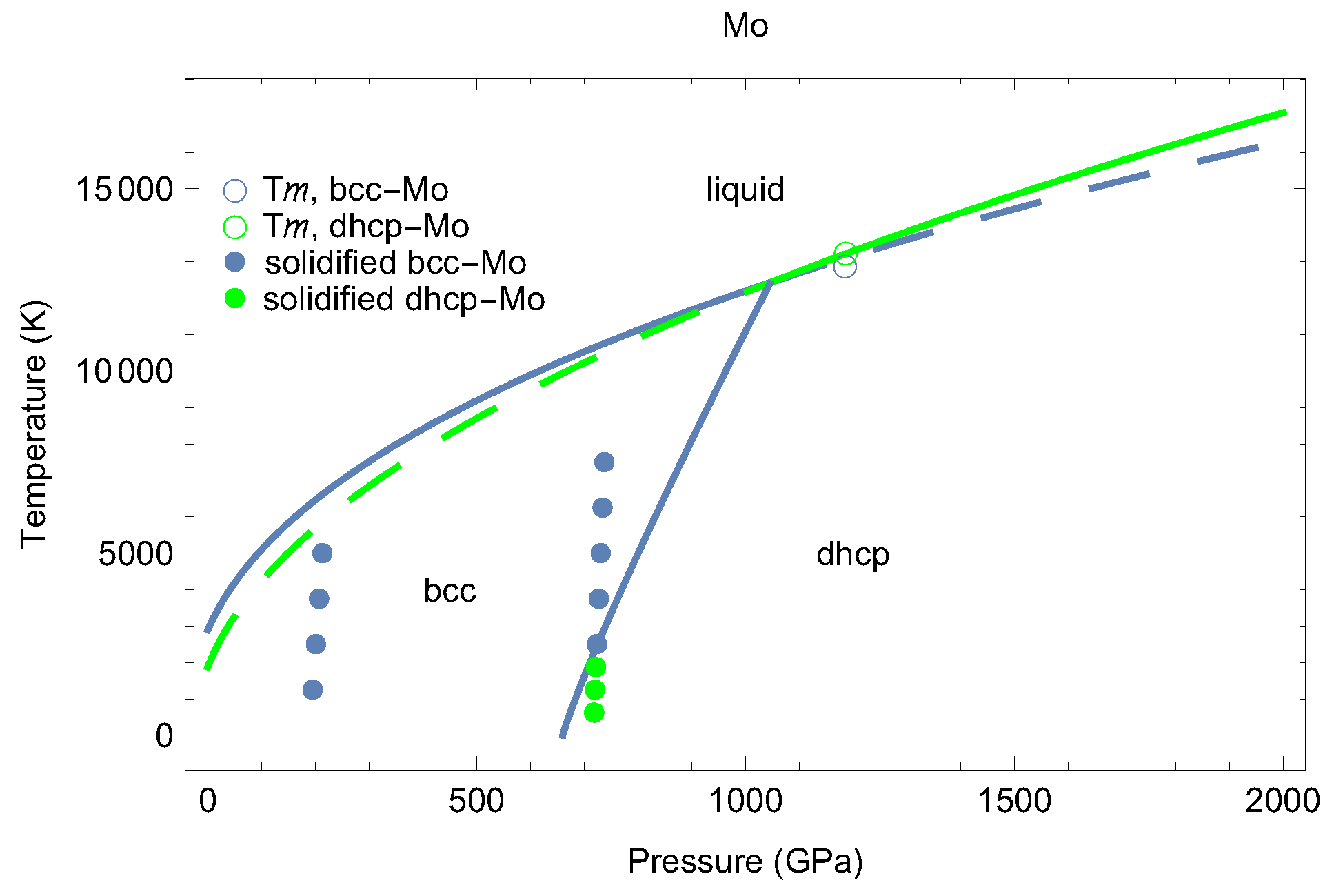
2. The Phase Diagram of Mo

The construction of the phase diagram of Mo using state-of-the-art theoretical techniques was discussed in detail in Reference [39], where we presented the phase diagram of Mo to 800 GPa. Here, we extend this phase diagram to 2000 GPa by calculating the melting curve of the double hexagonal close-packed (dhcp) structure of Mo, which is the stable solid phase of Mo at $P\ge 660$ GPa [39], and by determining the solid–solid phase transition boundary between the body-centered cubic (bcc) structure, which is the stable solid phase of Mo at $P\le 660$ GPa, and the dhcp structure. Our results can be summarized as follows:

(i)

the melting curve of bcc-Mo in the Simon–Glatzel form [40] ($T_m$ in K, P in GPa):

$$T_m\left(P\right)=2896{\left(1+\frac{P}{36.6}\right)}^{0.43},$$

(1)

(ii)

the melting curve of dhcp-Mo in the Simon–Glatzel form ($T_m$ in K, P in GPa):

$$T_m\left(P\right)=1880{\left(1+\frac{P}{24.5}\right)}^{0.50},$$

(2)

Our melting curve of bcc-Mo, Equation (1), is in excellent agreement with another theoretical calculation, $T_m\left(P\right)=2894{(1+P/37.2)}^{0.433}$ [41]. For Equation (1), $d{T}_m{/dP|}_{P=0}=34.0$ K/GPa, which is in excellent agreement with 32 K/GPa [26] or $34\pm 6$ K/GPa [42], each from isobaric expansion measurements.

Figure 1 and Figure 2 demonstrate the time evolution of T and $P$, respectively, in the Z method runs of the bcc-Mo melting point (P in GPa, T in K) $(P,T)$ = (1185, 12,770), which is one of the melting points that we calculated in the course of the present study. Figure 3 and Figure 4 demonstrate the same for the dhcp-Mo melting point (1186, 13,430). These two points are chosen as examples and are shown in Figure 5 as open blue and green circles, respectively.

The melting curves of bcc-Mo and dhcp-Mo cross each other at (P in GPa, T in K) $(P,T)=$ (1045, 12,320) which is the bcc–dhcp-liquid triple point. The choice of $T\left(P\right)=a{(660-P)}^b,0<b<1$ as a functional form for the bcc–dhcp phase boundary leads to

(iii) the bcc–dhcp solid–solid phase transition boundary:

$$T\left(P\right)=58.5{(P-660)}^{0.90},$$

(3)

which crosses the triple point as well as the point $(P,T)=(725,2500)$ that comes from the solidification simulations using the inverse Z method; for more detail see Reference [39].

The phase diagram of Mo to 2000 GPa is shown in Figure 5. It includes the two melting curves, the solid–solid phase boundary, and the results of the solidification of liquid Mo into the final states of either solid bcc or solid dhcp using the inverse Z method. Figure 5 actually represents the extended version of Figure 11 of Reference [39] which covered a P range of 0–800 GPa.

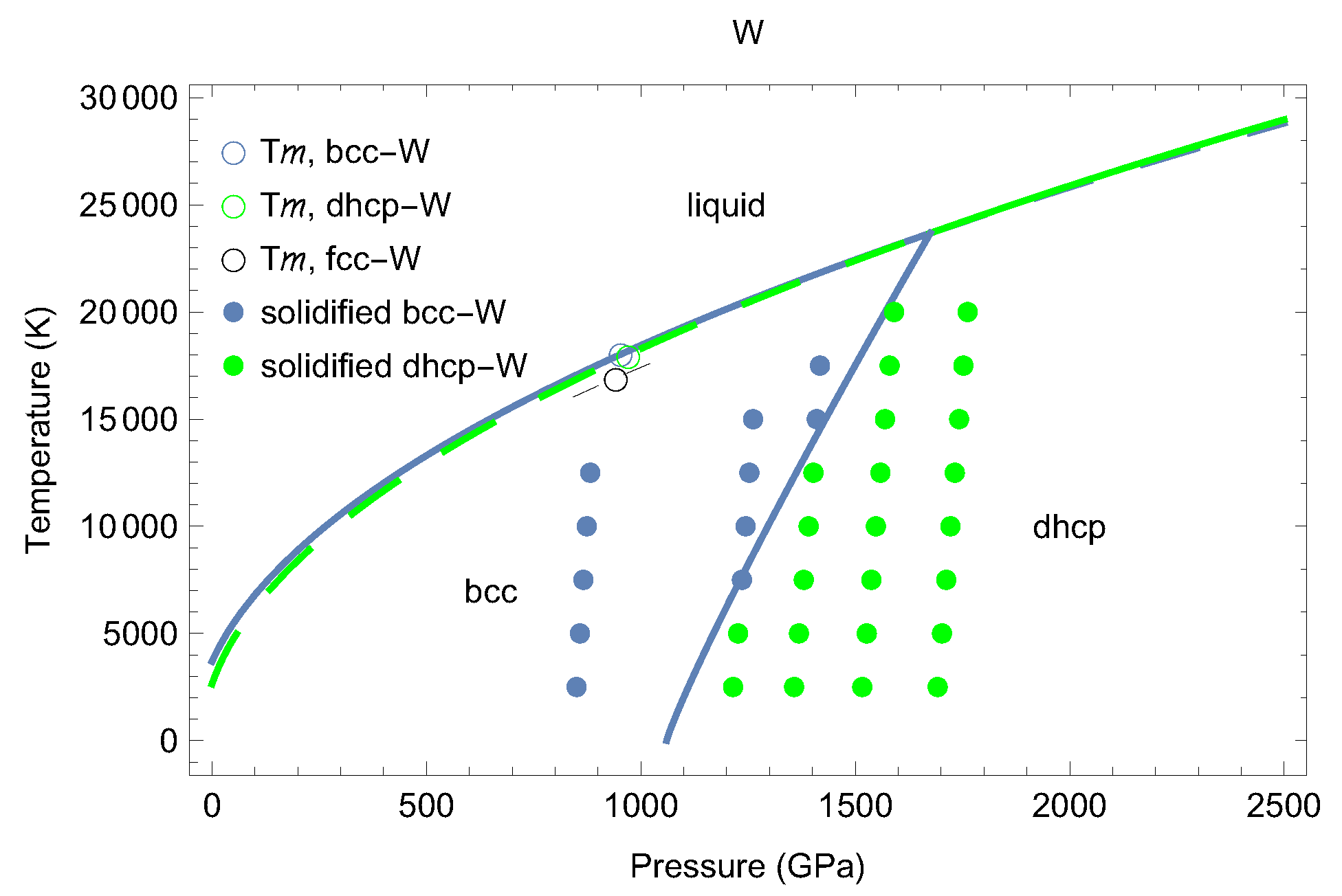
3. The Phase Diagram of W

Although the phase diagram of W has not been known in detail, there are several features of this phase diagram that have been firmly established. First, melting on the shock Hugoniot of W occurs at ∼400 GPa and presumably at $T\sim$12,000 K [27]; these values are extracted from the corresponding $P=P\left(U_p\right)$ and $T=T\left(U_p\right)$ dependences on the particle velocity $U_p$ as those at $U_p\sim 2.5$ km/s at which melting occurs on the shock Hugoniot of W [27]. Second, the stability of bcc-W has been confirmed experimentally under room-T isothermal compression to 420 GPa [43] and to 500 GPa [44]. There is presently no experimental evidence for an s–s transition in W. However, there is compelling theoretical evidence for an s–s phase transition at high $P.$ Calculations of the phonon spectra of both the bcc and face-centered cubic (fcc) structures of W show that bcc-W becomes mechanically unstable at pressures above 12 Mbar while fcc-W being mechanically unstable at low P becomes fully stabilized above 4 Mbar [45]. A very recent theoretical study [46] demonstrates that fcc-W becomes mechanically stable at ∼450 GPa while bcc-W becomes mechanically unstable with increasing $P$; above 12 Mbar, bcc-W is unstable at low T but remains stable above 1000 K. Hence, an s–s phase transformation to another solid phase that is mechanically stable is expected to occur at $P\stackrel{<}{\sim }12$ Mbar at low T and the s–s transition boundary is expected to have positive slope $(dT/dP>0)$ since the bcc-W stability range widens with increasing $T$. Because fcc-W also becomes thermodynamically more favorable than bcc-W [46], fcc-W is one of the candidates for the high-P solid structure of W. In fact, the bcc-fcc s–s phase transition was predictied to occur at ∼12 Mbar and calculations show that the bcc-fcc phase boundary does have positive slope at $P\ge 12$ Mbar [46]. However, in Reference [47], a transformation to a different solid structure, namely, dhcp, which is thermodynamically more stable than fcc, is predicted to occur, albeit at much lower pressure of 650 GPa. If a bcc–dhcp s–s phase transition does occur in W, just like in Mo, the two phase diagrams may look similar. As a matter of fact, as we demonstrate in what follows, the two phase diagrams are topologically equivalent.

We begin our theoretical study of the phase diagram of W with the calculation of the cold $(T=0)$ free energies (i.e., enthalpies) of a number of different solid structures of W as a function of $P$.

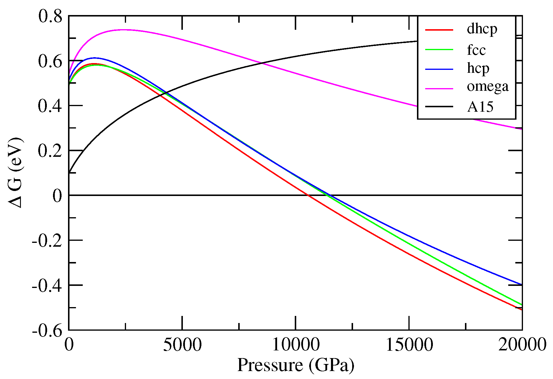
3.1. Cold Enthalpies of Different Solid Structures of W

The calculations were based on density-functional theory (DFT) with the projector-augmented wave (PAW) [48] implementation and the generalized gradient approximation (GGA) for exchange-correlation energy in the form known as Perdew–Burke–Ernzerhof (PBE) [49]. All the calculations were done using VASP (Vienna Ab initio Simulation Package). Since the simulations were performed at high-$PT$ conditions, we used accurate pseudopotentials where the semi-core 5s and 5p states were treated as valence states. Specifically, W was modeled with 14 valence electrons per atom (5s, 5p, 5d, and 6s orbitals). The valence electrons were represented with a plane-wave basis set with a cutoff energy of 500 eV, while the core electrons were represented by projector-augmented wave (PAW) pseudopotentials. The core radius (the largest value of RCUTs among those for each of the quantum orbitals) of this W pseudopotential is 2.3 a.u. or 1.217 Å. Since numerical errors in the calculations using VASP will remain almost negligible until the nearest neighbor distance reaches 2 × RCUT/$(1.25\pm 0.05)$ [39], with this pseudopotential, one can study systems with densities up to ∼80 g/cm³ (a pressure of ∼8000 GPa).

Cold enthalpies were calcualted using unit cells with very dense k-point meshes (e.g., $50\times 50\times 50$ for bcc-W) for high accuracy. In all the non-cubic cases, we first relaxed the structure to determine its unit cell parameters at each volume. Tight convergence criteria for the total energy $({10}^{-5}$ meV/atom) and structural relaxation (residual forces $<0.1$ meV/Å and stresses $\le 0.1$ kbar) were employed.

Our calculated cold enthalpies of five different solid structures of W are shown in Figure 6. It is seen that, with inceasing $P$, a number of other solid structures become thermodynamically more favorable than bcc, but it is dhcp that does it first, at a pressure of 1060 GPa, and remains the most favorable solid structure of W at higher $P$. Hence, in the case of W, the s–s transition boundary is the bcc–dhcp one and its starting point is $(P,T)=(1060,0)$.

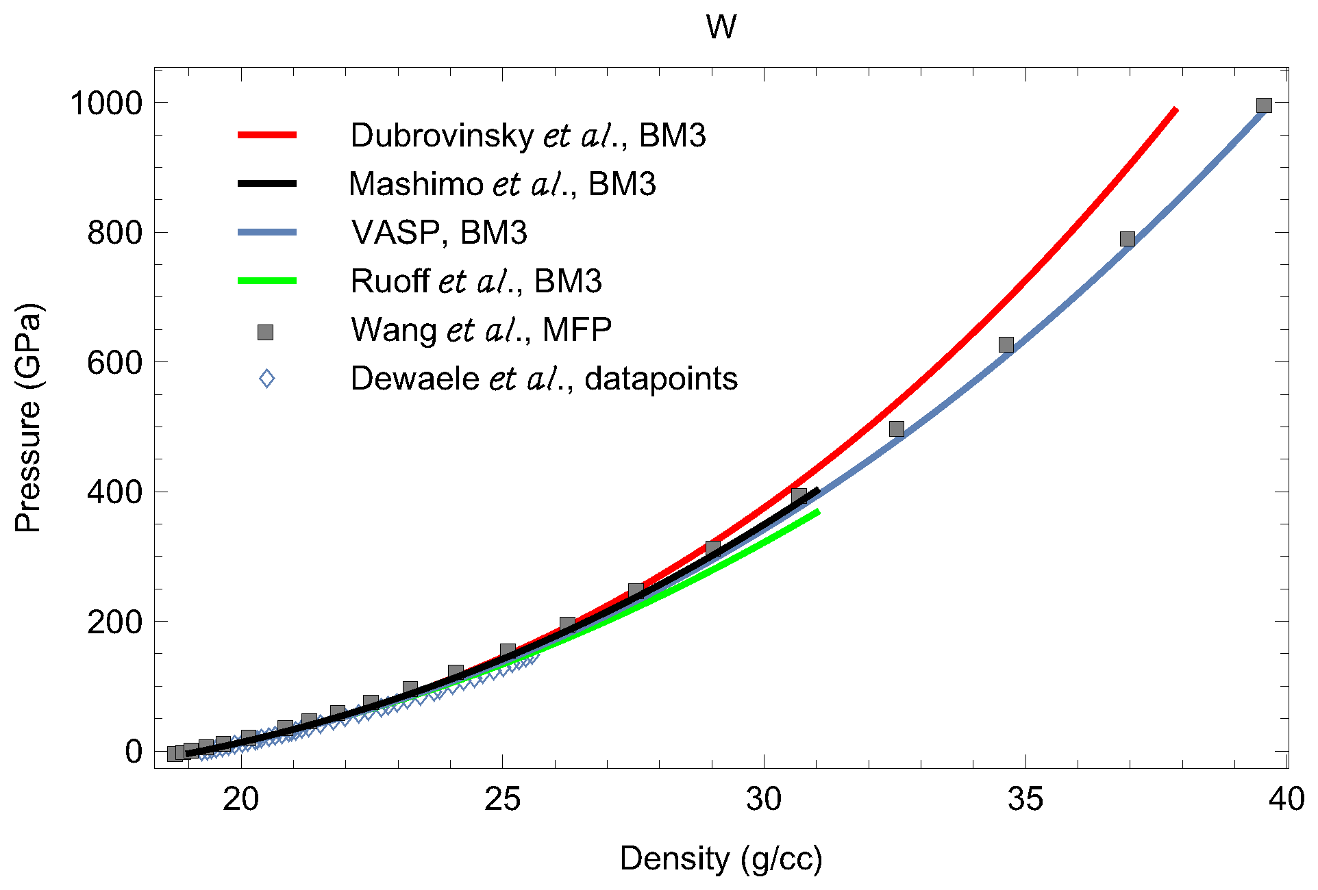
3.2. Equations of State of bcc-W and dhcp-W

Next, we calculate the cold equations of state of both bcc-W and dhcp-W. For dhcp-W, we also determine the density dependence of the $c/a$ ratio, where a and c are the lattice constants of the dhcp unit cell.

Our ab initio results on the cold equation of state (EOS) of bcc-W are described by the third-order Birch–Murnaghan (BM3) form:

$$P\left(\rho \right)=\frac{3}{2}{B}_0\left({\left(\frac{\rho }{{\rho }_0}\right)}^{7/3}-{\left(\frac{\rho }{{\rho }_0}\right)}^{5/3}\right)\left[1+\frac{3}{4}(B_0^{\prime }-4)\left({\left(\frac{\rho }{{\rho }_0}\right)}^{2/3}-1\right)\right],$$

(4)

where $B_0$ and $B_0^{\prime }$ are the values of the bulk modulus and its pressure derivative at the reference point $\rho ={\rho }_0.$ In our case of bcc-W,

$${\rho }_0=19.3{\mathrm{g}/\mathrm{cm}}^3,B_0=314.1\mathrm{GPa},B_0^{\prime }=4.07.$$

(5)

Since the $P=0$ values of the density of W at $T=0$ and 300 K differ by ∼0.3% (19.31 vs. 19.26 g/cc) and $T=300$ K introduces a negligibly small thermal pressure correction, the $T=0$ and $T=300$ K isotherms can be described by the same values of $B_0$ and $B_0^{\prime }$. Consequently, we can compare room-T isotherm data of References [44,50,51,52,53] to our $T=0$ isotherm as determined with VASP. A comparison is shown in Figure 7. It is seen that our EOS is virtually identical to the experimental isotherm of Reference [53], for which $B_0=317.5$ GPa and $B_0^{\prime }=4.05$ are very similar to ours, as well as to the theoretical calculations of Reference [51] in the so-called mean-field potential (MFP) approach.

For dhcp-W, the P dependence of the $c/a$ ratio for the lattice constants of the dhcp unit cell is accurately described by

$$\frac{c}{a}=3.2660-0.4912{\left(\frac{a}{a_0}\right)}^3+0.7484{\left(\frac{a}{a_0}\right)}^5,$$

(6)

where $a_0=2.8525$ Å coresponds to the ideal $(c/a=4\sqrt{2/3}\approx 3.2660)$ unit cell of the same reference density ${\rho }_0$ as that for the corresponding cold EOS. Since the unit cell volume is $c{a}^2\sqrt{3}/8$ $(a^3/\sqrt{2}$ for the ideal structure), the above relation can be translated into the P dependence of $c/a$ via the corresponding cold EOS of dhcp-W that we obtained. It is described by the BM3 form, Equation (4), with

$${\rho }_0=18.6{\mathrm{g}/\mathrm{cm}}^3,B_0=290.8\mathrm{GPa},B_0^{\prime }=3.95.$$

(7)

Above 1000 GPa, the dhcp-W structure is virtually ideal. At the transition pressure of 1060 GPa, the two density values predicted by these EOSs are (in g/cm³ 40.38 for bcc-W and and 40.53 for dhcp-W; hence, the bcc–dhcp transition corresponds to a small volume change of ∼0.4%.

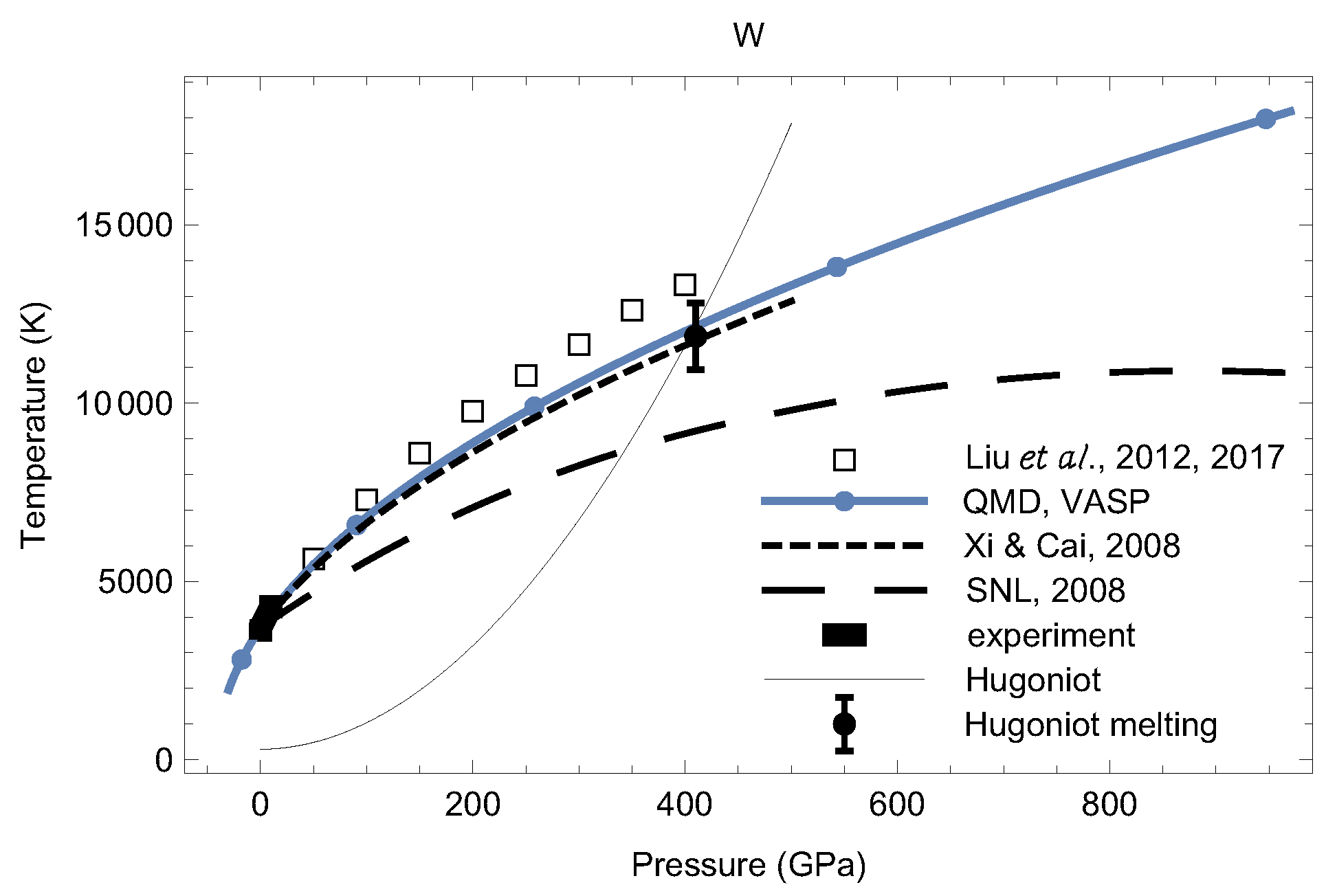
4. Melting Curves of Different Solid Structures of W

We now discuss the calculation of the melting curves of different solid structures of W. For this calculation, we used the Z method, which is described in detail in References [9,36,54]. We calculated the melting curves of bcc-W as well as a number of other solid structures of W which have been mentioned in the literature in connection with transition metals: all the close-packed structures with different layer stacking (fcc, hcp, dhcp, thcp, and 9R), open structures (simple cubic, A15, and hex-$\omega$), and different orthorhombic structures (Pnma, Pbca, Pbcm, Cmca, Cmcm, etc.). Again, in all the non-cubic cases, we relaxed the structure to determine its unit cell parameters; those unit cells were used for the construction of the corresponding supercells. We used systems of 400–500 atoms in each case.

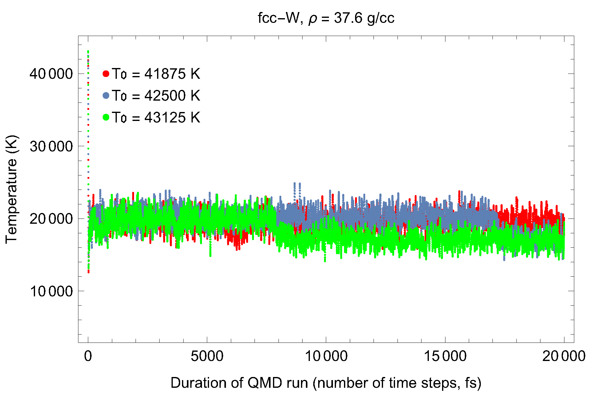
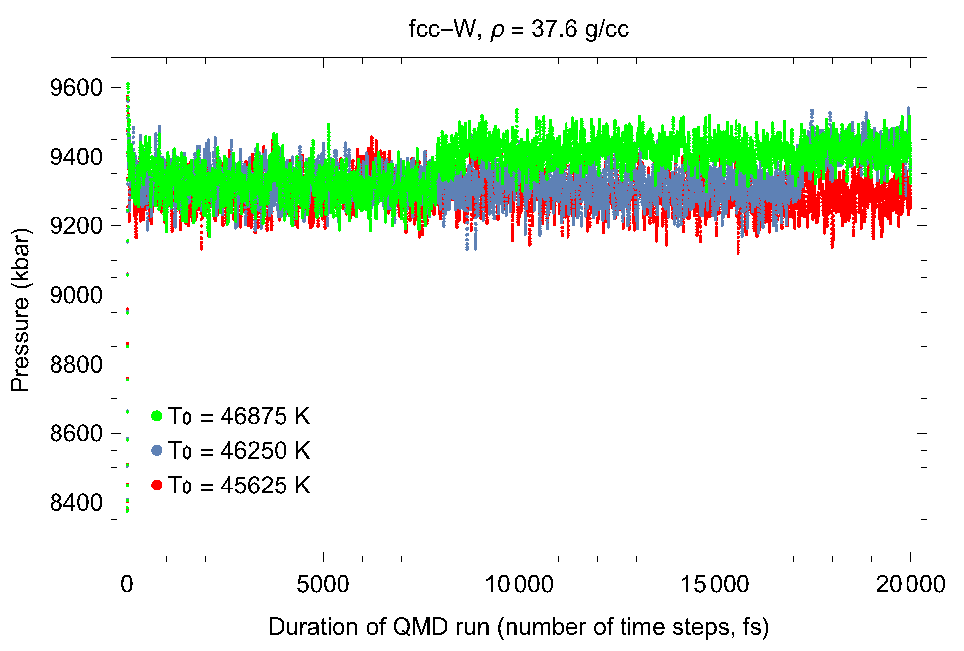
4.1. Ab Initio Melting Curve of bcc-W

For the calculation of the melting curve of bcc-W (with the Z method), we used a 432-atom ($6\times 6\times 6$) supercell with a single $\mathsf{\Gamma }$-point. Full energy convergence (to $\stackrel{<}{\sim }1$ meV/atom) was verified by performing short runs with $2\times 2\times 2$ and $3\times 3\times 3$ k-point meshes and by comparing their output with that of the run with a single $\mathsf{\Gamma }$-point. For each of the five points listed in

Table 1. The five ab initio melting points of bcc-W, $(P_m,T_m\pm \Delta T_m)$, obtained from the Z method implemented with VASP.

Lattice Constant (Å)	Density (g/cm3)	${\mathit{P}}_{\mathit{m}}$ (GPa)	${\mathit{T}}_{\mathit{m}}$ (K)	$\mathbf{\Delta }{\mathit{T}}_{\mathit{m}}$ (K)
3.350	16.240	−17.7	2800	125.0
3.050	21.519	90.6	6520	312.5
2.850	26.375	258	9840	312.5
2.675	31.897	543	13,760	312.5
2.535	37.479	947	18,070	312.5

, we performed ten $NVE$ runs (five values of V correspond to five values of densities in Table 1) of 10,000–20,000 time steps of 1 fs each, with an increment of the initial T of 250 K for the first datapoint and 625 K for the remaining four. Since the error in T is half of the increment [36], the T errors of our five values of $T_m$ are within 5% each. The P errors are negligibly small: less than 1 GPa for the first point and 1–2 GPa for the remaining four. Hence, our melting results on bcc-W are very accurate.

The best fit to the five bcc-W melting points gives the melting curve of bcc-W in the Simon–Glatzel form ($T_m$ in K, P in GPa):

$$T_m\left(P\right)=3695{\left(1+\frac{P}{41.8}\right)}^{0.50}.$$

(8)

Its initial slope, $d{T}_m\left(P\right)/dP=44.2$ K/GPa at $P=0,$ is in excellent agreement with 44 K/GPa from isobaric expansion measurements [26]. Both the five bcc-W melting points and the melting curve (Equation (8)) are shown in Figure 8 and compared to the experimental results in Reference [27,30], the calculated Hugoniot of W [55], and other theoretical calculations [6,56,57,58].

4.2. Ab Initio Melting Curve of dhcp-W

The five melting points of dhcp-W that we obtained are listed in

Table 2. The five ab initio melting points of dhcp-W, $(P_m,T_m\pm \Delta T_m),$ obtained from the Z method implemented with VASP: The lattice constant values correspond to the ideal dhcp structure.

Lattice Constant (Å)	Density (g/cm3)	${\mathit{P}}_{\mathit{m}}$ (GPa)	${\mathit{T}}_{\mathit{m}}$ (K)	$\mathbf{\Delta }{\mathit{T}}_{\mathit{m}}$ (K)
2.90	17.702	8.1	3080	150.0
2.65	23.199	150	7380	312.5
2.40	31.230	510	13,110	312.5
2.25	37.902	970	18,000	312.5
2.15	43.440	1471	22,200	312.5

. The dhcp-W melting simulations were carried out exactly the same way as the bcc ones, namely, 10 runs per point, 10,000–20,000 time steps of 1 fs each per run, and an increment of the initial T of 300 K for the first datapoint and 625 K for the remaining four. Just as for bcc-W, a 432-atom ($6\times 6\times 3$) supercell was used to simulate each of the five dhcp-W melting points. Also, as for bcc-W, the T errors of our five values of $T_m$ are within 5% each.

The best fit to the five dhcp-W points gives the melting curve of dhcp-W in the Simon–Glatzel form ($T_m$ in K, P in GPa):

$$T_m\left(P\right)=2640{\left(1+\frac{P}{23.0}\right)}^{0.51}.$$

(9)

Figure 9 and Figure 10 demonstrate the time evolution of T and $P,$ respectively, in the Z-method runs of the bcc-W melting point (P in GPa, T in K) $(P,T)=(947,18,070).$ Figure 11 and Figure 12 demonstrate the same for the dhcp-W melting point $(970,18,000).$ These two points are chosen as examples and are shown in Figure 13 as open blue and green circles, respectively.

All the other solid structures that we considered melt below bcc. As an example, one of the fcc-W melting points, namely, $(P,T)=$ (942, 16,920), along with a short segment of the corresponding melting curve, are shown in Figure 13. The corresponding time evolution of T and P in the Z-method runs are shown in Figure 14 and Figure 15, respectively.

The melting curves of bcc-W and dhcp-W cross each other at (P in GPa, T in K) $(P,T)=$ (1675, 23,680), which is the bcc–dhcp-liquid triple point. The choice of $T\left(P\right)=a{(1060-P)}^b,0<b<1$ as a functional form for the bcc–dhcp phase boundary leads to

(iii) the bcc–dhcp solid–solid phase transition boundary:

$$T\left(P\right)=73.2{(P-1060)}^{0.90},$$

(10)

which crosses the triple point and lies within the bounds imposed by the solidification simulations using the inverse Z method. We discuss these inverse Z simulations in the following section.

Although the rigorous derivation of the thermal equations of state of bcc-W and dhcp-W goes beyond the scope of this work, we note that the finite-T counterparts of the above two EOSs can be written approximately as $P(\rho ,T)=P\left(\rho \right)+\alpha T,$ where ${\alpha }_{\mathrm{bcc}}=7.3$ × ${10}^{-3}$ and ${\alpha }_{\mathrm{dhcp}}=6.8$ × ${10}^{-3}.$ The resulting “approximate” thermal EOSs turn out to be quite accurate. For example, for the five bcc-W melting points in Table 1, the corresponding thermal EOS gives pressures of −17.8, 90.3, 258, 543, and 948, which are basically identical to those in the third column of Table 1. For the five dhcp-W melting points in Table 2, the five P values are 7.9, 150, 509, 970, and 1476, in excellent agreement with those in the third column of Table 2.

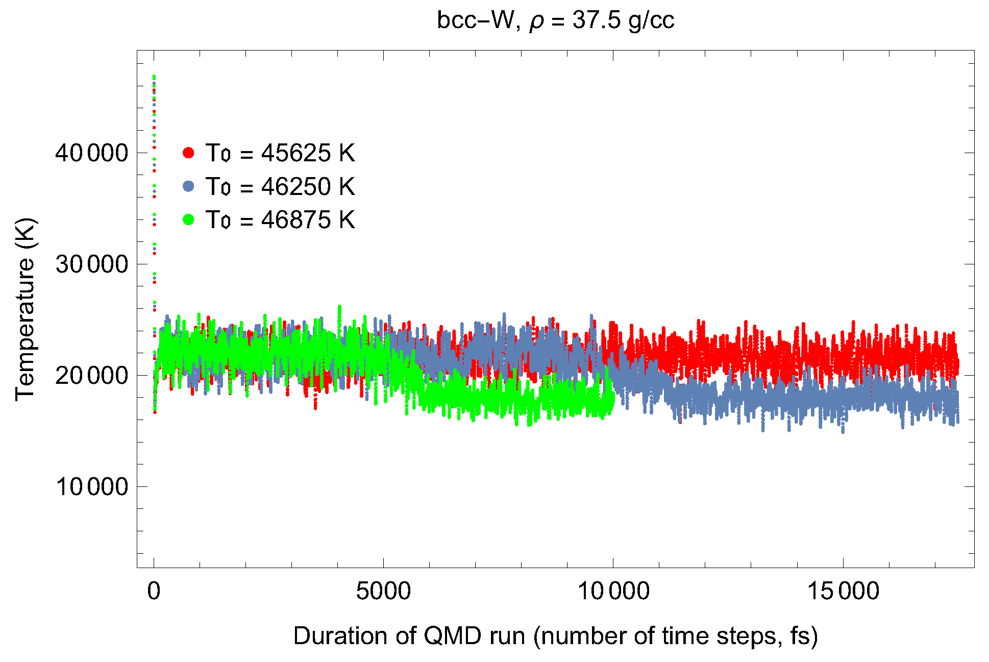
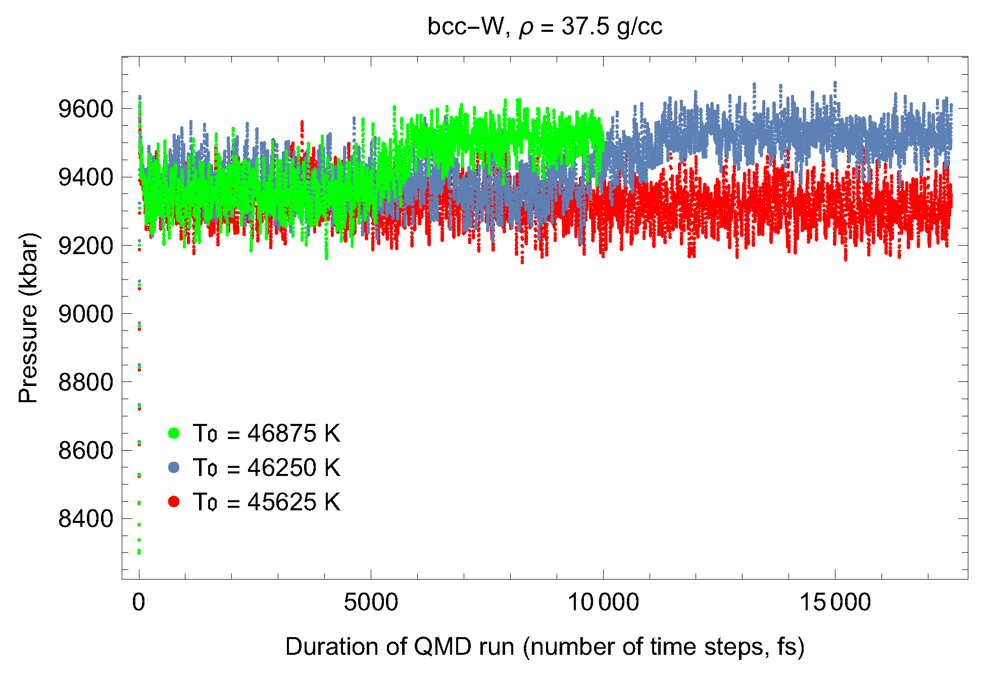
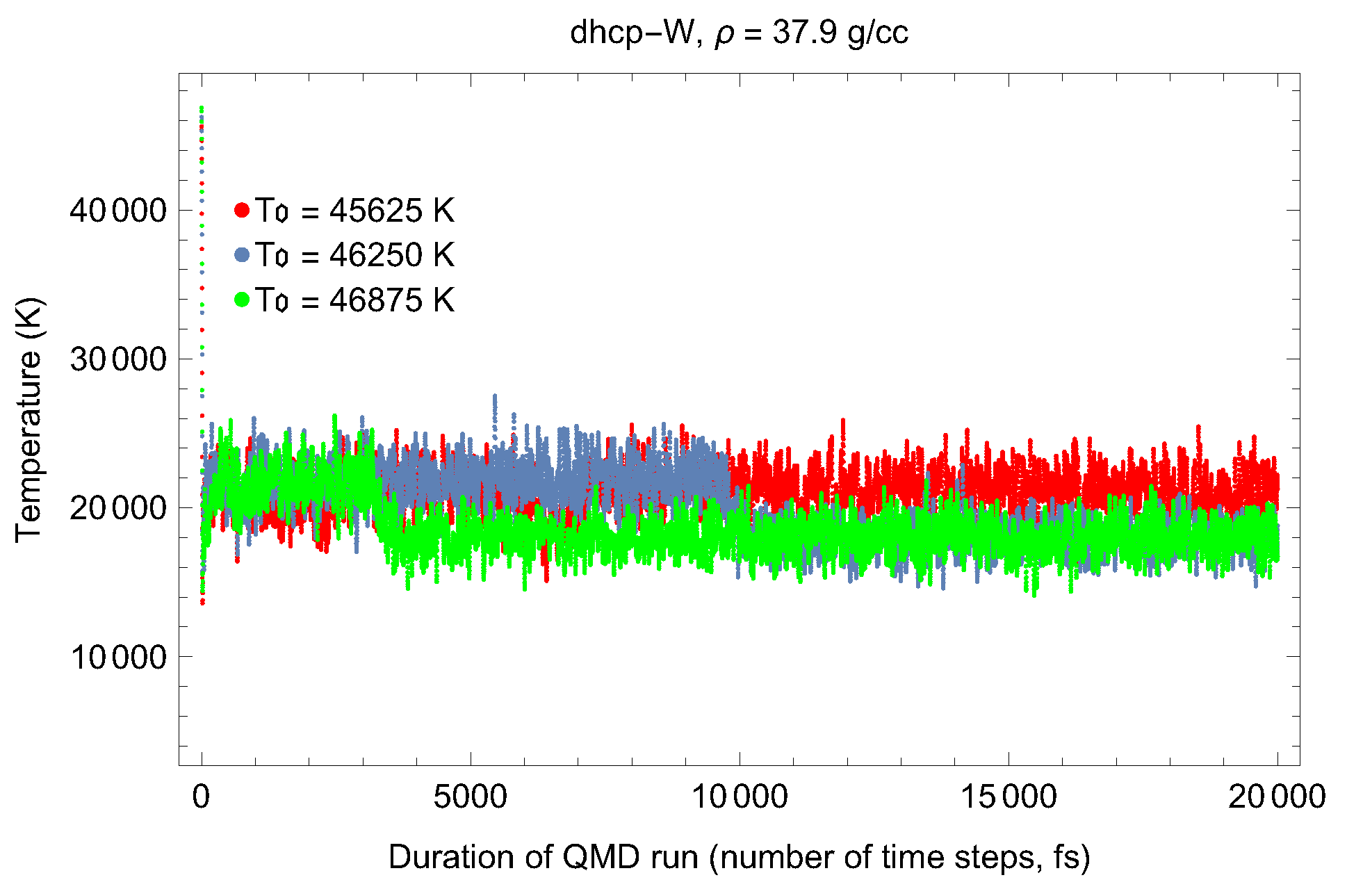
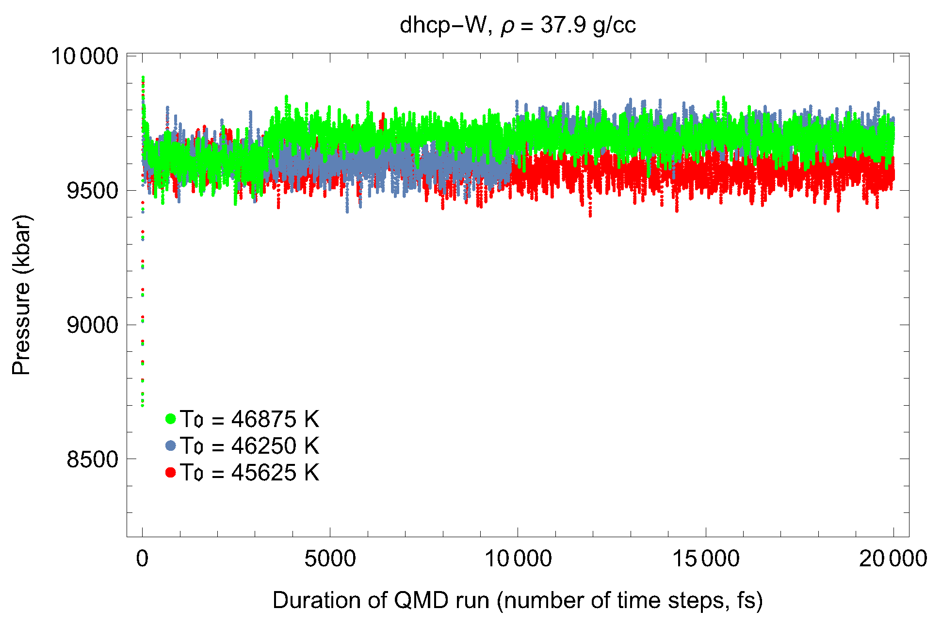
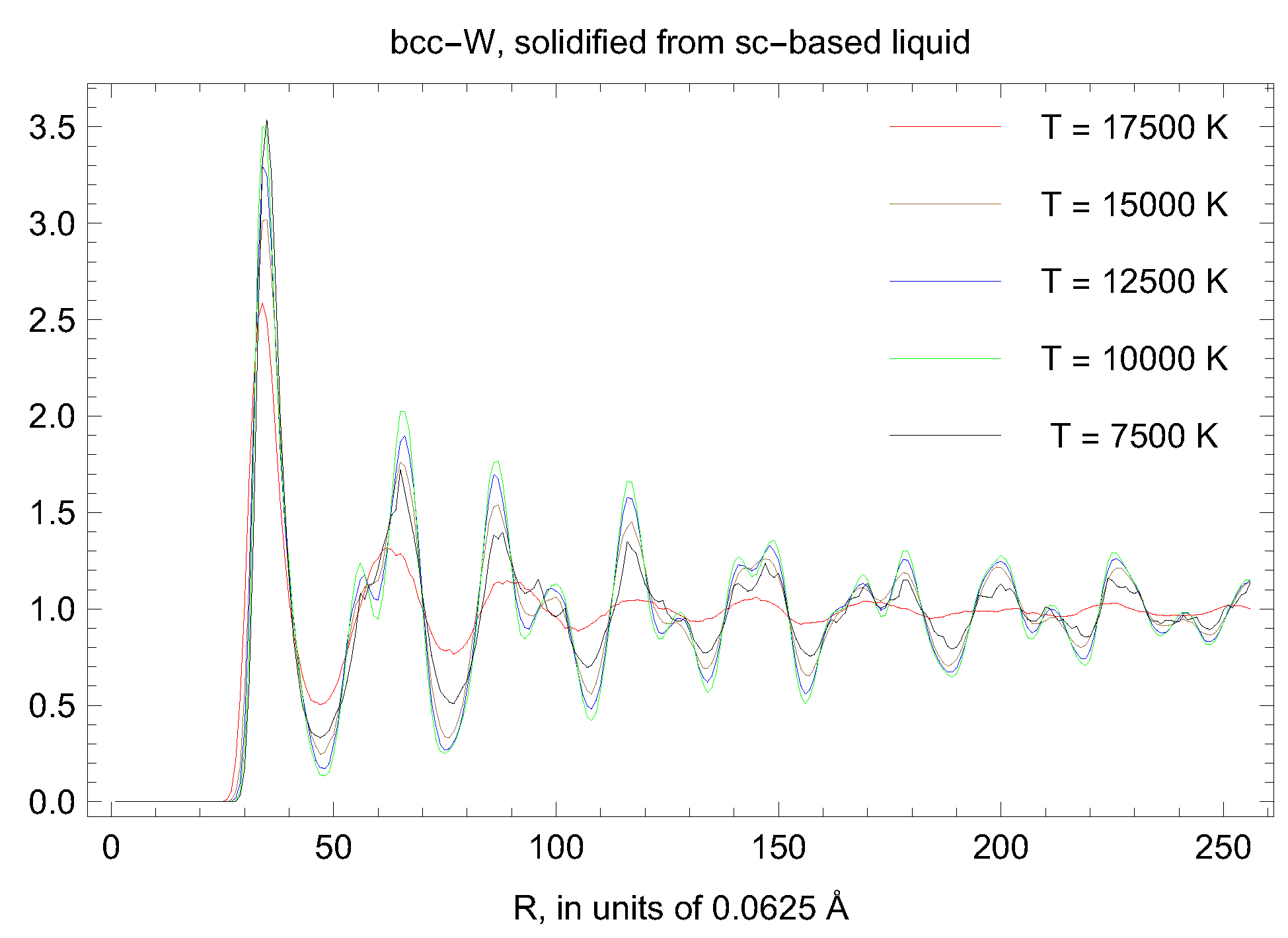
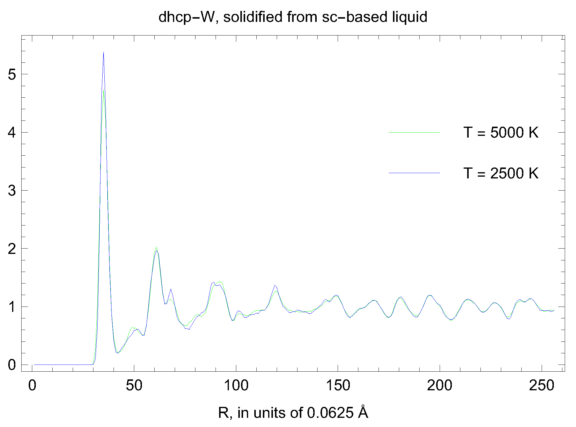
5. Inverse Z Solidification Simulations of Liquid W

To constrain the location of the bcc–dhcp solid–solid phase boundary on the P–T plane between the points $(P=1060,T=0)$ and (P = 1675, T = 23,680), we carried out two sets of independent inverse Z runs [9] to solidify liquid W and to confirm that liquid W solidifies into bcc on one side of this boundary and into dhcp (or any other solid structure) on the other side, such that the location of this phase boundary may be constrained. Since the solidification kinetics is approximately governed by the factor $exp\{\Delta F/T^{*}\},$ where $\Delta F\equiv F_l-F_s$ is the liquid–solid free-energy difference at the solidification temperature $T^{*},$ in the case of several energetically competitive solid phases, the most thermodynamically favorable solid phase has the largest $\Delta F$ and is therefore the fastest to solidify. Hence, the inverse Z method yields the most stable solid phase at a given $(P,T)$.

For our inverse Z simulations, we used a computational cell of 512 atoms prepared by melting a $8\times 8\times 8$ solid simple cubic (sc) supercell, which would eliminate any bias towards solidification into bcc or any other solid structure (fcc, hcp, dhcp, etc.). We used sc unit cells of 2.0, 1.935, 1.915, 1.895, and 1.870 Å; the dimensions of bcc unit cells having the same volume as the sc ones are 2.520, 2.438, 2.413, 2.388, and 2.356 Å, respectively, which corresponds to the bcc-W pressures of ∼870, 1225, 1355, 1505, and 1715 GPa and to slightly lower pressures for dhcp-W.

We carried out $NVT$ simulations using the Nosé–Hoover thermostat with a timestep of 1 fs, with the initial T increment of 2500 K. Complete solidification typically was required from 15 to 25 ps or 15,000–25,000 timesteps. The inverse Z runs indicate that liquid W only solidifies into bcc at ∼900 GPa in the whole temperature range from 0 to essentially the corresponding $T_m$. However, at ∼1200–1400 GPa, it solidifies into bcc above the transition boundary in Figure 13, while below this boundary, it solidifies into another solid structure. The radial distribution functions (RDFs) of the final solid states are noisy; upon fast quenching of the seven structures (seven green bullets in Figure 13 in the 1200–1400 GPa range) to low $T,$ where RDFs are more discriminating, and by comparing them to the RDFs of fcc, hcp, and dhcp, we conclude that dhcp is the closest strucure to those that liquid Mo solidies into below the transition boundary.

The RDFs of the solidified states at ∼1200 GPa above the transition boundary are shown in Figure 16 and of those solidified below the transition boundary are shown in Figure 17. The 7500 K state virtually lies on the boundary. We tentatively assign it to bcc because it definitely has features of bcc (RDF peaks at $R\sim 55$, 65, and 85, etc.). At the same time, it certainly has some features that are both uncharacteristic of bcc (e.g., the disappearance of the bcc peak at $R\sim 95$) and characteristic of dhcp (peaks at $R\sim 90$ and 120, small peaks at $R\sim 100$ and 130, etc.). Most likely, this 7500 K state is bcc with some admixture of dhcp.

A few more comments are in order. The 17,500 K state at ∼1250 GPa did not solidify, most likely for the reason of not being supercooled enough to intiate the solidification process [9]. Indeed, 17,500 K constitutes ∼0.8 of the corresponding $T_m$ of ∼22,000 K (20% of supercooling) while, e.g., for the other set of points at ∼900 GPa, the highest solidification T of 12,500 K constitutes ∼0.75 of the corresponding $T_m$ of ∼17,000 K (25% of supercooling), which apparently allows for the solidification process to go through in this case.

The phase diagram of W to 2500 GPa is shown in Figure 13. It includes the two bcc and dhcp melting curves, the bcc–dhcp solid–solid phase transition boundary, and the results of the solidification of liquid W into final states of either solid bcc or solid dhcp using the inverse Z method.

Both the Mo and W phase diagram figures, Figure 5 and Figure 13, do not show the previous experimental DAC melting curves of Errandonea et al. [13,16] and are both flat, with the initial slope of ∼7–8 K/GPa. We did not include those in the two figures because we do not consider them to be relevant. The very recent experimental study by Hrubiak et al. [23] demonstrates that, on increasing $T,$ compressed Mo undergoes a transformation that results in a texture (microstructure) change: large Mo grains become unstable at high T due to high atom mobility and reorganize into smaller crystalline grains. This transformation occurs below melting, and the pressure dependence of the transformation temperature is consistent with the previous DAC melting curve by Errandonea et al. [13]. Hence, most likely, Errandonea’s curve is an intermediate DAC transition boundary, while our curve as well as Alfe’s [41], which is basically identical to ours, is the actual melting curve of Mo.

A behavior similar to that of Mo (a texture change) was recently observed in the high-$PT$ melting experiments on V [25]. Hence, this phenomenon of a texture (microstructure) change can be common to a number of transition metals, including W. It is therefore natural to assume that, in the case of W, too, the corresponding Errandonea’s melting curve is an intermediate DAC transition boundary while our curve is the actual melting curve of W.

6. Concluding Remarks

The phase diagrams of Mo and W, Group 6B partners in the periodic table, shown in Figure 5 and Figure 13, respectively, are topologically equivalent. In both cases, the ambient bcc solid structure transforms into dhcp on increasing $P$. Only these two solid phases are confirmed as being present on the two phase diagrams, via ab initio QMD simulations using the Z methodology. Even the critical aspect ratio of the two phase diagrams is identical. Indeed, the ratio of the pressure values for the bcc–dhcp-liquid triple point and the $T=0$ bcc–dhcp transition (it determines the curvatures and the locus of the bcc–dhcp transition boundary on the P–T plnae) is the same in both cases: 1045/660 = 1.583 for Mo and 1675/1060 = 1.580 for W. The two transition boundaries, Equations (3) and (10), are described by the same exponent 0.9 which further confirms the topological equivalence of the two phase diagrams.

It is interesting to note another case of the phase diagrams of Nb and Ta, group 5B partners in the periodic table, which appear to be topologically similar (look-alike) but not equivalent. In both cases, a bcc-Pnma solid–solid phase transition occurs [9,59], but in contrast to dhcp in Mo and W, the orthorhombic Pnma phase exists at high T only. In Ta, the bcc-Pnma-liquid triple point is at a pressure which is an order of magnitude higher than that in Nb [9,59]. Also, the bcc-Pnma transition T increases with P in Nb but decreases with T in Ta.

Inverse Z solidification simulations confirm the phase diagrams of Mo and W shown in Figure 5 and Figure 13, respectively, and validate the corresponding bcc–dhcp solid–solid phase boundaries. Additional support for the existence of the high-P dhcp structure in both Mo and W comes from Reference [60]. The electronic wave functions of Mo and W and of their group 5B partner Cr are such that, with decreasing volume (increasing P), they become more spherically symmetric, which favors a higher atomic coordination number than 8 as that for bcc and, correspondingly, a more symmetric structure than bcc. It is well known that the highest possible coordination number is 12, and it corresponds to all of the hexagonal polytypes, namely, hcp (stacking sequence $AB$), fcc ($ABC$), dhcp ($ABAC$), triple-hcp ($ABCACB$), etc. It is therefore natural to expect that, at high P, both Mo and W and perhaps Cr as well will have one of the hexagonal polytypes as their equilibrium solid structure. Our study demonstrates that this polytype is in fact dhcp. It is interesting to note that, in Cr, as theoretical calculations show [61], hcp becomes energetically more favorable than bcc with decreasing volume (increasing P). Since different hexagonal polytypes are usually close to each other energetically, one can therefore expect them to be the high-P equilibrium solid structure of Cr. Thus, it is quite possible that the phase digram of Cr is topologically similar, if not equivalent, to those of both Mo and W. In contrast to both Mo and W, the study of Reference [62] shows that the electronic wave functions of V, Nb, and Ta are such that, with decreasing volume, they become less spherically symmetric, which favors a lower atomic coordination number than bcc’s 8 and, correspondingly, a less symmetric structure than bcc, e.g., an orthorhombic one. This appears to be in agreement with the fact that, in both Nb and Ta, the high-P equilibrium solid structure is orthorhombic Pnma.

Fast recrystallization observed in HP-HT experiments on transition metals may imply either a microstructural transition (discussed above) at which the sample texture changes but its crystal structure remains the same or a true solid–solid phase transition. The former was recently proven to be the case in Mo [23], and it is very likely the case in V [25] as well as in W. The latter is apparently the case in Nb [59] and likely in Re as well [10]. In either case, the corresponding fast recrystallization lines have been misinterpreted as flat melting curves in the former laser-heating DAC experiments.

References

1. Belonoshko, A.B.; Burakovsky, L.; Chen, S.P.; Johansson, B.; Mikhaylushkin, A.S.; Preston, D.L.; Simak, S.I.; Swift, D.C. Molybdenum at high pressure and temperature: Melting from another solid phase. Phys. Rev. Lett. 2008, 100, 135701. [Google Scholar] [CrossRef] [PubMed]
2. Liu, Z.-L.; Cai, L.-C.; Chen, X.-R.; Jing, F.-Q. Molecular dynamics simulations of the melting curve of tantalum under pressure. Phys. Rev. B 2008, 77, 024103. [Google Scholar] [CrossRef]
3. Burakovsky, L.; Chen, S.P.; Preston, D.L.; Belonoshko, A.B.; Rosengren, A.; Mikhaylushkin, A.S.; Simak, S.I.; Moriarty, J.A. High-pressure–high-temperature polymorphism in Ta: Resolving an ongoing experimental controversy. Phys. Rev. Lett. 2010, 104, 255702. [Google Scholar] [CrossRef] [PubMed]
4. Haskins, J.; Moriarty, J.A.; Hood, R.Q. Polymorphism and melt in high-pressure tantalum. Phys. Rev. B 2012, 86, 224104. [Google Scholar] [CrossRef] [Green Version]
5. Hu, J.; Dai, C.; Yu, Y.; Liu, Z.; Tan, Y.; Zhou, X.; Tan, H.; Cai, L.; Wu, Q. Sound velocity measurements of tantalum under shock compression in the 10–110 GPa range. J. Appl. Phys. 2012, 111, 033511. [Google Scholar] [CrossRef] [Green Version]
6. Liu, C.M.; Chen, X.R.; Xu, C.; Cai, L.C.; Jing, F.Q. Melting curves and entropy of fusion of body-centered cubic tungsten under pressure. J. Appl. Phys. 2012, 112, 013518. [Google Scholar] [CrossRef]
7. Yao, Y.; Klug, D. Stable structures of tantalum at high temperature and high pressure. Phys. Rev. B 2013, 88, 054102. [Google Scholar] [CrossRef]
8. Pozzo, M.; Alfe, D. Melting curve of face-centered-cubic nickel from first-principles calculations. Phys. Rev. B 2013, 88, 024111. [Google Scholar] [CrossRef] [Green Version]
9. Burakovsky, L.; Chen, S.P.; Preston, D.L.; Sheppard, D.G. Z methodology for phase diagram studies: Platinum and tantalum as examples. J. Phys. Conf. Ser. 2014, 500, 162001. [Google Scholar] [CrossRef] [Green Version]
10. Burakovsky, L.; Burakovsky, N.; Preston, D.; Simak, S.I. Systematics of the third row transition metal melting: The hcp metals rhenium and osmium. Crystals 2018, 8, 243. [Google Scholar] [CrossRef] [Green Version]
11. Lazor, P.; Shen, G.; Saxena, S.K. Laser-heated diamond anvil cell experiments at high pressure: Melting curve of nickel up to 700 kbar. Phys. Chem. Miner. 1993, 20, 86. [Google Scholar] [CrossRef]
12. Kavner, A.; Jeanloz, R. High-pressure melting curve of platinum. J. App. Phys. 1998, 83, 7553. [Google Scholar] [CrossRef]
13. Errandonea, D.; Schwager, B.; Ditz, R.; Gessmann, C.; Boehler, R.; Ross, M. Systematics of transition-metal melting. Phys. Rev. B 2001, 63, 132104. [Google Scholar] [CrossRef]
14. Errandonea, D.; Somayazulu, M.; Häusermann, D.; Mao, H.K. Melting of tantalum at high pressure determined by angle dispersive x-ray diffraction in a double-sided laser-heated diamond-anvil cell. J. Phys. Cond. Mat. 2003, 15, 7635. [Google Scholar] [CrossRef]
15. Boehler, R.; Santamaría-Perez, D.; Errandonea, D.; Mezouar, M. Melting, density, and anisotropy of iron at core conditions: New X-ray measurements to 150 GPa. J. Phys. Conf. Ser. 2008, 121, 022018. [Google Scholar] [CrossRef]
16. Santamaría-Pérez, D.; Ross, M.; Errandonea, D.; Mukherjee, G.D.; Mezouar, M.; Boehler, R. X-ray diffraction measurements of Mo melting to 119 GPa and the high pressure phase diagram. J. Chem. Phys. 2009, 130, 124509. [Google Scholar] [CrossRef] [Green Version]
17. Ruiz-Fuertes, J.; Karandikar, A.; Boehler, R.; Errandonea, D. Microscopic evidence of a flat melting curve of tantalum. Phys. Earth Planet. Inter. 2010, 181, 69. [Google Scholar] [CrossRef] [Green Version]
18. Yang, L.; Karandikar, A.; Boehler, R. Flash heating in the diamond cell: Melting curve of rhenium. Rev. Sci. Instrum. 2012, 83, 063905. [Google Scholar] [CrossRef]
19. Dewaele, A.; Mezouar, M.; Guignot, N.; Loubeyre, P. High melting points of tantalum in a laser-heated diamond anvil cell. Phys. Rev. Lett. 2010, 104, 255701. [Google Scholar] [CrossRef] [Green Version]
20. Errandonea, D. High-pressure melting curves of the transition metals Cu, Ni, Pd, and Pt. Phys. Rev. B 2013, 87, 054108. [Google Scholar] [CrossRef]
21. Anzellini, S.; Dewaele, A.; Mezouar, M.; Loubeyre, P.; Morard, G. Melting of iron at Earth’s inner core boundary based on fast X-ray diffraction. Science 2013, 340, 464. [Google Scholar] [CrossRef] [PubMed]
22. Lord, O.T.; Wood, I.G.; Dobson, D.P.; Vočadlo, L.; Wang, W.; Thomson, A.R.; Wann, E.T.; Morard, G.; Mezouar, M.; Walter, M.J. The melting curve of Ni to 1 Mbar. Earth Planet. Sci. Lett. 2014, 408, 226. [Google Scholar] [CrossRef] [Green Version]
23. Hrubiak, R.; Meng, Y.; Shen, G. Microstructures define melting of molybdenum at high pressures. Nat. Commun. 2017, 8, 14562. [Google Scholar] [CrossRef] [PubMed] [Green Version]
24. Anzellini, S. In situ characterization of the high pressure–high temperature melting curve of platinum. Sci. Rep. 2019, 9, 13034. [Google Scholar] [CrossRef] [PubMed] [Green Version]
25. Errandonea, D.; MacLeod, S.G.; Burakovsky, L.; Santamaria-Perez, D.; Proctor, J.E.; Cynn, H.; Mezouar, M. Melting curve and phase diagram of vanadium under high-pressure and high-temperature conditions. Phys. Rev. B 2019, 100, 094111. [Google Scholar] [CrossRef] [Green Version]
26. Shaner, J.W.; Gathers, G.R.; Minichino, C. A new apparatus for thermophysical measurements above 2500 K. High Temp.-High Pres. 1976, 8, 425. [Google Scholar]
27. Hixson, R.S.; Fritz, J.N. Shock compression of tungsten and molybdenum. J. Appl. Phys. 1992, 71, 1721. [Google Scholar] [CrossRef]
28. Musella, M.; Ronchi, C.; Sheindlin, M. Dependence of the melting temperature on pressure up to 2000 bar in uranium dioxide, tungsten, and graphite. Int. J. Thermophys. 1999, 20, 1177. [Google Scholar] [CrossRef]
29. Kloss, A.; Hess, H.; Schneidenbach, H.; Grossjohann, R. Scanning the melting curve of tungsten by a submicrosecond wire-explosion experiment. Int. J. Thermophys. 1999, 20, 1199. [Google Scholar] [CrossRef]
30. Gustafson, P. Evaluation of the thermodynamic properties of tungsten. Int. J. Thermophys. 1985, 6, 395. [Google Scholar] [CrossRef]
31. Vereshchagin, L.F.; Fateeva, N.S. Melting curves of graphite, tungsten and platinum to 60 kbar. Sov. Phys. JETP 1969, 28, 597. [Google Scholar]
32. Gorecki, T. Vacancies and melting curve of metals at high pressure. Z. Metallk. 1977, 68, 231. [Google Scholar]
33. Gorecki, T. Vacancies and a generalised melting curve of metals. High Temp.-High Press. 1979, 11, 683. [Google Scholar]
34. Arblaster, J.W. What is the true melting point of osmium? Platin. Met. Rev. 2005, 49, 166. [Google Scholar] [CrossRef]
35. Zitserman, V.; (JIHT, Moscow). Personal communication. 2019. [Google Scholar]
36. Burakovsky, L.; Burakovsky, N.; Preston, D.L. Ab initio melting curve of osmium. Phys. Rev. B 2015, 92, 174105. [Google Scholar]
37. Burakovsky, L.; Preston, D.L. Shear moduli of silicon and germanium in semiconducting and metallic phases. Defect Diffus. Forum 2002, 210–212, 43. [Google Scholar] [CrossRef]
38. Frohberg, M.G. Thirty years of levitation melting calorimetry-a balance. Thermochem. Acta 1999, 337, 7. [Google Scholar] [CrossRef]
39. Burakovsky, L.; Lushcer, D.J.; Preston, D.; Sjue, S.; Vaughan, D. Generalization of the unified analytic melt-shear model to multi-phase materials: Molybdenum as an example. Crystals 2019, 9, 86. [Google Scholar] [CrossRef] [Green Version]
40. Simon, F.; Glatzel, G. Bemerkungen zur Schmelzdruckkurve. Z. Anorg. Allgem. Chem. 1929, 178, 309. [Google Scholar] [CrossRef]
41. Cazorla, C.; Gillan, M.J.; Taioli, S.; Alfè, D. Melting curve and Hugoniot of molybdenum up to 400 GPa by ab initio simulations. J. Phys. Conf. Ser. 2008, 121, 012009. [Google Scholar] [CrossRef] [Green Version]
42. Shaner, J.W.; Gathers, G.R.; Minichino, C. Thermophysical properties of liquid tantalum and molybdenum. High Temp.-High Press. 1977, 9, 331. [Google Scholar]
43. Ruoff, A.L.; Xia, H.; Xia, Q. The effect of a tapered aperture on x-ray diffraction from a sample with a pressure gradient: Studies on three samples with a maximum pressure of 560 GPa. Rev. Sci. Instrum. 1992, 63, 4342. [Google Scholar] [CrossRef]
44. Dubrovinsky, L.; Dubrovinskaia, N.; Bykova, E.; Bykov, M.; Prakapenka, V.; Prescher, C.; Glazyrin, K.; Liermann, H.-P.; Hanfland, M.; Ekholm, M.; et al. The most incompressible metal osmium at static pressures above 750 gigapascals. Nature 2015, 525, 226. [Google Scholar] [CrossRef] [PubMed]
45. Einarsdotter, K.; Sadigh, B.; Grimvall, G.; Ozoliņš, V. Phonon instabilities in fcc and bcc tungsten. Phys. Rev. Lett. 1997, 79, 2073. [Google Scholar] [CrossRef] [Green Version]
46. Zhang, H.-Y.; Niu, Z.-W.; Cai, L.-C.; Chen, X.-R.; Xi, F. Ab initio dynamical stability of tungsten at high pressures and high temperatures. Comput. Mater. Sci. 2018, 144, 32. [Google Scholar] [CrossRef]
47. Ruoff, A.L.; Rodriguez, C.O.; Christensen, N.E. Elastic moduli of tungsten to 15 Mbar, phase transition at 6.5 Mbar, and rheology to 6 Mbar. Phys. Rev. B 1998, 58, 2998. [Google Scholar] [CrossRef]
48. Blöchl, P. Projector augmented-wave method. Phys. Rev. B 1994, 50, 17953. [Google Scholar] [CrossRef] [Green Version]
49. Perdew, J.P.; Burke, K.; Ernzerhof, M. Generalized gradient approximation made simple. Phys. Rev. Lett. 1996, 77, 3865. [Google Scholar] [CrossRef] [Green Version]
50. Ruoff, A.L.; Xia, H.; Luo, H.; Vohra, Y.K. Miniaturization techniques for obtaining static pressures comparable to the pressure at the center of the earth: X-ray diffraction at 416 GPa. Rev. Sci. Instrum. 1990, 61, 3830. [Google Scholar] [CrossRef]
51. Wang, Y.; Chen, D.; Zhang, X. Calculated equation of state of Al, Cu, Ta, Mo, and W to 1000 GPa. Phys. Rev. Lett. 2000, 84, 3220. [Google Scholar] [CrossRef]
52. Dewaele, A.; Loubeyre, P.; Mezouar, M. Equations of state of six metals above 94GPa. Phys. Rev. B 2004, 70, 094112. [Google Scholar] [CrossRef] [Green Version]
53. Mashimo, T.; Liu, X.; Kodama, M.; Zaretsky, E.; Katayama, M.; Nagayama, K. Effect of shear strength on Hugoniot-compression curve and the equation of state of tungsten (W). J. Appl. Phys. 2016, 119, 035904. [Google Scholar] [CrossRef]
54. Belonoshko, A.B.; Skorodumova, N.V.; Rosengren, A.; Johansson, B. Melting and critical superheating. Phys. Rev. B 2006, 73, 012201. [Google Scholar] [CrossRef]
55. McQueen, R.G.; Marsh, S.P. Equation of state for nineteen metallic elements from shock-wave measurements to two megabars. J. Appl. Phys. 1960, 31, 1253. [Google Scholar] [CrossRef]
56. Xi, F.; Cai, L. Theoretical study of melting curves on Ta, Mo, and W at high pressures. Phys. B 2008, 403, 2065. [Google Scholar] [CrossRef]
57. Carpenter, J.H.; Desjarlais, M.P.; Mattsson, A.E.; Cochrane, K.R. A New Wide-Range Equation of State for Tungsten; SNL Report SAND2008-1415C; American Physical Society: Washington, DC, USA, 2008. [Google Scholar]
58. Liu, C.M.; Xu, C.; Cheng, Y.; Chen, X.R.; Cai, L.C. Molecular dynamics studies of body-centered cubic tungsten during melting under pressure. Chin. J. Phys. 2017, 55, 2468. [Google Scholar] [CrossRef]
59. Errandonea, D.; Burakovsky, L.; Preston, D.L.; MacLeod, S.G.; Santamaría-Perez, D.; Chen, S.P.; Cynn, H.; Simak, S.I.; McMahon, M.L.; Proctor, J.E.; et al. Niobium at High Pressure and High Temperature: Combined Experimental and Theoretical Study. 2019; submitted. [Google Scholar]
60. Xie, Y.-Q.; Deng, Y.-P.; Liu, X.-B. Electroic structure and physical properties of pure Cr, Mo and W. Trans. Nonferrous Met. Soc. China 2003, 13, 5. [Google Scholar]
61. Pure Chromium. Available online: https://icme.hpc.msstate.edu/mediawiki/index.php/Pure_Chromium (accessed on 30 December 2019).
62. He, Y.; Xie, Y.-Q. Electroic structure and properties of V, Nb and Ta metals. J. Cent. South Univ. Technol. 2000, 7, 7. [Google Scholar] [CrossRef]
Figure 1. Time evolution of temperature for body-centred cubic (bcc) Mo in three QMD runs with initial temperatures (T0s) separated by 625 K: The middle run is the melting run, during which T decreases from ∼17,000 K for the superheated state to ∼12,800 K for the liquid at the corresponding melting point.
Crystals 10 00020 g001
Figure 2. The same as in Figure 1 for the time evolution of pressure (in kbar; 10 kbar = 1 GPa): During melting, P increases from ∼1180 GPa for the superheated state to ∼1185 GPa for the liquid state at the corresponding melting point.
Crystals 10 00020 g002
Figure 3. The same as in Figure 1 for double hexagonal close-packed (dhcp) Mo.
Crystals 10 00020 g003
Figure 4. The same as in Figure 2 for dhcp-Mo.
Crystals 10 00020 g004
Figure 5. Ab initio phase diagram of molybdenum.
Crystals 10 00020 g005
Figure 6. The T = 0 free energies of different solid structures of W (listed in the legend) from ab initio calculations using VASP (Vienna Ab initio Simulation Package): The free energy of bcc-W is taken to be identically zero.
Crystals 10 00020 g006
Figure 7. The T = 0 equation of state of bcc-W: our own ab initio calculations using VASP vs. experimental data (Dubrovinsky et al. [44]; Ruoff et al. [50]; Dewaele et al. [52]; and Mashimo et al. [53]) and other theoretical calculations (Wang et al. [51]).
Crystals 10 00020 g007
Figure 8. The melting curve of bcc-W: QMD simulations using VASP vs. other theoretical calculations (Xi an Cai [56]; SNL, 2008 [57]; and Liu et al., 2012 [6] and 2017 [58]), the low-pressure melting data (experiment in Reference [30]), and the experimental shock melting datapoint (Hugoniot melting [27]). The calculated Hugoniot is shown as a thin black curve.
Crystals 10 00020 g008
Figure 9. The same as in Figure 1 for bcc-W.
Crystals 10 00020 g009
Figure 10. The same as in Figure 2 for bcc-W.
Crystals 10 00020 g010
Figure 11. The same as in Figure 1 for dhcp-W.
Crystals 10 00020 g011
Figure 12. The same as in Figure 2 for dhcp-W.
Crystals 10 00020 g012
Figure 13. Ab initio phase diagram of tungsten.
Crystals 10 00020 g013
Figure 14. The same as in Figure 1 for fcc-W.
Crystals 10 00020 g014
Figure 15. The same as in Figure 2 for fcc-W.
Crystals 10 00020 g015
Figure 16. Radial distribution functions (RDFs) of the final states of the solidification of liquid W at ∼1200 GPa at higher temperatures.
Crystals 10 00020 g016
Figure 17. RDFs of the final states of the solidification of liquid W at ∼1200 GPa at lower temperatures.
Crystals 10 00020 g017