Abstract
This paper presents an order reduction for the thermal dynamics of a diesel oxidation catalyst (DOC) with hydrocarbon (HC) dosing. The original model includes the pyrolysis of diesel droplets and a wall storage process in the upstream of the DOC. The order reduction process is derived from the thermodynamics model of the DOC for further control design. The results are compared with experimental data. It is found that the DOC can be simplified as a second-order model using the HC dosing model, which has more than 94% fitness, reflecting the thermodynamics of the system. According to this research, the DOC thermal dynamics can be considered to be equivalent to a time-varying second-order system for the investigation. The second-order parameters of K, Tw, and ζ are also investigated in this paper.
1. Introduction
With increasingly stringent emission regulations, researchers widely paid attention to diesel after-treatment. Diesel after-treatment thermal management, which is an effective way to satisfy the stringent emission regulations, was researched for years. In the emission control of a diesel engine, the diesel oxidation catalyst (DOC), diesel particulate filter (DPF), and selective catalyst reduction (SCR) were integrated to eliminate hydrocarbons (HCs), particulate matter (PM), and nitrogen oxides (NOx) [1]. DPF, which has a porous structure to filter the PM, needs a suitable temperature to be activated. The temperature is nearly 600 °C without a catalyst [2]. However, the diesel engine does not generate this temperature during normal operation. Furthermore, NO needs to be oxidized to NO2 for the purpose of improving the elimination of PM inside DPF. The oxidation is more efficient when the exhaust is above 340 °C [3]. SCR, which is used to reduce NOx emissions, needs a temperature of 300–400 °C to ensure the reaction efficiency under most conditions [4]. However, the light-duty condition only generates a low temperature exhaust, inducing a low efficiency of catalytic reactions. For these reasons, researchers found a way to heat up the exhaust by increasing the concentration of hydrocarbons under oxygen-rich conditions [5]. In the heating-up process, hydrocarbons react in the DOC and release heat into the exhaust. This method can make the exhaust satisfy the necessary temperature requirements.
The widely implemented ways of increasing HCs are post-injection in the cylinder and HC dosing in the upstream of the DOC. Post-injection in the cylinder involves adding an extra injection after the normal diesel injection. This method has various advantages, such as a simple structure and low cost; thus, engineers based many works on it [6]. However, its shortcoming, i.e., that it induces lubricating oil dilution, is also obvious [7]. By comparison, HC dosing, which involves mounting a doser in the upstream of the DOC and generating a diesel droplet spray, has no impact on the diesel engine performance. Moreover, it is convenient for upgrading an in-use vehicle. Therefore, it is meaningful to study the thermodynamics of the DOC with HC dosing.
For a basic understanding of the coupled flow and chemical reaction in the catalyst, many researchers gradually constructed and perfected the basic model of catalytic thermal dynamics [8,9,10]. Researchers applied these models to investigate the thermodynamics of hydrocarbon addition in the DOC. Oh proposed a transient model to analyze the thermal effects of exhaust parameters in the DOC [11]. Groppi investigated a lumped model [12]. For further investigation on the exothermic reaction inside the DOC, researchers investigated the mechanism of the hydrocarbon catalytic reaction. The global kinetics for the C3H6 catalytic reaction on a platinum catalyst using the Langmuir–Hinshelwood (LH) form was first proposed by Voltz [13]. On this basis, most subsequent models for the DOC chemical reaction were extended from this form. For further investigation of the reaction species, Kryl divided the hydrocarbons into three species to investigate the effects of the exhaust parameters [14]. Sampara and Bissett proposed a reaction model with two hydrocarbons and predicted the conversion ratio [15,16]. According to recent researches, the kinetics of the catalytic reaction inside the DOC was gradually clarified [17,18,19,20,21]. However, kinetics is complex, and it is hard to apply in actual engineering and control. Hence, control-oriented models were proposed by researchers for simplification [22]. Benaicha proposed a time-delay reduced model and developed two model-based controllers [23]. Chen proposed a control-oriented simplified temperature dynamic model for in-cylinder post-injection [24]. The model considered the influence of the post-injection rate and timing. A state-space form dynamic model was proposed in the investigation. Donkers proposed an optimal control for diesel after-treatment thermal management [25]. In the control model, they reduced a third-order engine after-treatment system (EAS) model to a second-order model.
Some results on diesel thermal management control design can be found in the literature. The results show that the physical and chemical model of diesel after-treatment thermal management is hard to directly apply to actual engineering. Hence, the order reduction of the DOC thermodynamics from the physical field to control the field is a general trend. In the investigations of other researchers, various model reduction works for the thermodynamics of the DOC were given. However, in these investigations, the reduced model was only oriented toward the corresponding control strategy design. Furthermore, the theoretical basis and the validation were not given in some papers. Hence, the versatility of these reduced models is slightly inadequate. On the basis of these works, we made some innovations in relation to the complete order-reduction process. In our investigation, a relatively logical demonstration of the reduction process is given. Meanwhile, our reduction is from a DOC thermodynamics model, which is a complex fluid problem, to a second-order transfer function. The second-order characteristics are very general in the control region. Hence, the investigation can help expand the control strategy for a diesel exhaust heating system, such as an adaptive Proportion Integration Differentiation (PID) control, robust control, and optimal control. In this paper, a problem description and the primary model are proposed in Section 2.1. The second-order derivation and the reduction from DOC thermodynamics are proposed in Section 2.2 and Section 2.3. Based on this derivation, an experiment is conducted under different conditions, with different dosing parameters. The experimental set-up and design are shown in Section 3. The identification method and identification results are shown in Section 4. At the end of the paper, conclusions are given.
2. Thermodynamics of the DOC Using an HC Doser
2.1. Problem Description and Primary Model
The exhaust heating system is composed of an HC doser, the DOC, and the exhaust of a diesel engine. The investigation concerns the thermal performance of the DOC with diesel droplet oxidation inside. The HC doser is located downstream of the exhaust gas recirculation (EGR), which is the inlet of the DOC. After dosing, the diesel droplets are directly injected into the exhaust flow. These droplets continuously evaporate and are converted to gaseous hydrocarbon species in the gas phase. Then, the species are absorbed by the active sites on the surface of the DOC substrate via mass diffusion before reacting. The process is shown in Figure 1.
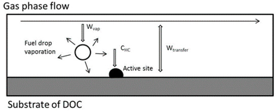
Figure 1.
Schematic of the diesel droplet oxidation inside the diesel oxidation catalyst (DOC).
After the catalytic reaction, the hydrocarbon species are converted to carbon dioxide and water in the active sites. Then, products are released to the gas phase. The reaction is an exothermic reaction. Hence, the DOC substrate and exhaust are heated up by the exothermic process and reach the target temperature for DPF regeneration or some other utilization. The model of DOC thermal dynamics with post-injection was proposed by researchers [22]. Compared with previous models, the DOC thermal dynamics models using an HC doser have some differences. The diesel droplets, which are at room temperature, are injected into a hot exhaust. Hence, the heating up and thermolysis of the droplets need to be considered inside the DOC. The assumptions about the model are as follows:
- (1)
- The model is a one-dimensional model, which is uniform in the radial direction;
- (2)
- The species, such as NOx, HC, and CO, in the original exhaust are eliminated, because the order of the magnitude is less than the effect of the dosing species;
- (3)
- The heat conduct term is eliminated, because Pe > 50, according to the investigation of Lepreux [22];
- (4)
- The endothermic effect of the droplet evaporation is eliminated in the gaseous energy balance, because the order of magnitude is less than the exothermic effect of the catalytic reaction.
These assumptions are reasonable under general diesel engine conditions. In the exhaust pipe of the DOC, the airflow is uniform in the radial direction. Hence, a one-dimensional model for the DOC reaction is widely used by researchers. The concentration of the dosing species is more than 15,000 ppm for the heating-up exhaust. As for the original species, the concentration is lower than 1000 ppm under all conditions; thus, the original species can be eliminated in the diesel exhaust heating model. The reason for eliminating the conduct term of the DOC model is given in Lepreux’s research [22]. For the evaporation of diesel droplets, the endothermic effect is only 4.64 × 10⁴ J/mol, which can only generate a 1–5-K fluctuation in the exhaust temperature. However, the chemical reaction of hydrocarbons has an exothermic effect of more than 4.0 × 10⁶ J/mol, which is 100 times more than the evaporation effect. As a result, the endothermic effect of the droplet evaporation is eliminated in the gaseous energy balance. For more details of the energy balance and mass balance inside the DOC, readers can refer to prior investigations [13,14,15,16,17,18,19,20,21,22]. The model is proposed as follows:
Energy balance:
Mass balance:
where subscript s refers to the solid phase, and subscript g refers to the gas phase. Ci,g is the molar fraction of species i in the gas phase, ε is the porosity of the DOC, F is the mass flow rate of the exhaust, km,i is the mass transfer coefficient, S is the geometric surface area-to-volume ratio, aPt is the catalytic surface area-to-volume ratio (volume represents the volume of the control unit), ri is the rate of the reaction of species i, Acell is the mean cell cross-sectional area, λg is the thermal conductivity of gas, ht is the convective heat transfer coefficient between the gas and solid, cp is the specific heat, ΔHk is the enthalpy of chemical species k, and aPt’ is the amount of catalyst coating.
The chemical reaction includes gaseous reactions and solid-phase reactions. Compared with in-cylinder post-injection, gaseous reactions are specific in this system. In this paper, gaseous reactions adopt the model, proposed by Ning, with some changes [26]. The reason is that, in the actual thermolysis process of diesel, small-molecule hydrocarbons vaporize first. Hence, the thermolysis is divided into two steps, considering the actual diesel fuel thermolysis and evaporation. Meanwhile, stoichiometry rebalances, considering the main species C7H8 in diesel fuel l (DF1) and C10H22 in diesel fuel 2 (DF2).
The catalytic reaction in the solid phase of the DOC was investigated by researchers for years. The reaction is shown in Equations (7)–(9).
The gaseous reaction reflects the thermolysis and evaporation of diesel fuel droplets. The reaction is a continuous vaporization process for small-molecule hydrocarbons. Hence, it can be treated as a decomposition process. The decomposition rate is expressed by the Arrhenius form in Equations (10) and (11).
In the equations, rliq is the reaction rate of the first step of thermolysis (Equation (5)), reflecting the generation rate of C3H6 (DVF) and diesel residue. Furthermore, rresid is the reaction rate of the second step of thermolysis (Equation (6)), reflecting the generation rate of DF1 and DF2. Aliq is the pre-exponential factor of Equation (5). Eliq is the activation energy of Equation (5). Cliq is the gaseous species concentration of diesel fuel in Equation (5). Similarly, Aresid is the pre-exponential factor of Equation (6). Eresid is the activation energy of Equation (6). Cresid is the gaseous species concentration of diesel residue in Equation (6). Finally, n in Equations (10) and (11) represents the reaction order of diesel fuel thermolysis. It requires identification using experimental calibration.
Considering the reaction rate in the solid phase of the DOC, the LH form is widely used in DOC investigations [13,14,15,16,17,18,19,20]. The chemical kinetics of the DOC, proposed by Kryl [14], were recognized by researchers [15,16,17,18,19,20]. Hence, in this paper, the rate model is adopted, with some changes. It is shown in Equations (12)–(14).
In Equations (12)–(14), rs,C3H6 is the reaction rate of C3H6 on the surface of the catalyst, rs,DF1 represents the surface reaction rate of DF1, and rs,DF2 represents the rate of DF2. The numerator term reflects the reaction rate, which contains the pre-exponential factor, activation energy, and molar concentrations of the reactants. The denominator is the coverage of the adsorbed species in the LH equations. The Arrhenius form is also adopted in the denominator term. The pre-exponential factor and activation energy in the inhibitory term are usually treated as correction factors. These factors are identified by calibration.
2.2. Order Reduction of Energy Balance
The order reduction is based on the energy balance equations of the primary model. Two simplified factors, proposed by Lepreux [22] (k1 and k2), are adopted. After consolidation and simplification, the equations are as follows:
where T(x,t) refers to the temperature in the axial position of x at time t, and Φ(x,t) refers to the energy source term of the hydrocarbon reaction. The source term can be simplified, as shown in the following section. The boundary conditions of the temperature in the time dimension and space dimension are defined as Equation (17), according to experimental data. Based on the boundary conditions of the model, a real-time temperature can be divided into two parts, as shown in Equation (18), where Tg_noinj(x,t) and Ts_noinj(x,t) represent the temperature with no dosing. Tg_noinj(x,t) and Ts_noinj(x,t) are only influenced by the working condition parameters. The net temperature induced by HC dosing is written as ΔTg(x,t) and ΔTs(x,t). In the following equations, our main purpose is to research the characteristics of the net temperature induced by HC dosing.
On the basis of the above equations, Equations (15) and (16) are transformed into the Laplace form as follows:
τ(x,s) is defined as a convolution function and is used for the simplification of the space derivative as follows:
The Laplace form of the above equation is
τ(x,s) is a factor that represents the difference between ∂ΔTg/∂x and ΔTg/x. We assume that the difference between ∂ΔTg/∂x and ΔTg/x does not change much in the heating process. Thus, the difference can be treated as a supplementary constant β(x) to be expressed. The physical meaning of β(x) is the ratio of the net temperature gradient to the net temperature slope. This is shown in Equation (22).
Hence, Equation (19) is transformed into
According to the definition, the relationship between Tg and φ is a second-order linear transfer function under some conditions, in which it has little variation in the exhaust flow rate and little variation in β(x). In general, in the heating-up process, the relation is a second-order time-varying process. Simultaneously, the linear form of Ts is shown in Equation (24).
From the equations, the net temperature of the exhaust is simplified as a second-order system with two poles. In comparison, the net temperature of the DOC substrate is a second-order system with two poles and one zero. The addition of the zero will induce a faster heating-up process in the DOC substrate than in the gas phase. The result is identical with the actual thermal dynamics of the DOC heating-up process. Equation (24) can be written as follows:
where K is an amplification coefficient, which reflects the conversion ability of the reaction heat to the exhaust net temperature. A higher K induces a higher net temperature, with the same source term of energy. Tw is a time coefficient, which reflects the time required to reach a steady state. A higher Tw induces a longer time to reach a steady state of the system. ζ is a damping ratio, which reflects the stability and resistance of the system. A higher ζ induces greater resistance in the heating-up and cooling-down processes but less overshoot in stability. The three factors define a second-order system. The solid phase has a similar form; thus, it is eliminated. In this reduction, the thermal dynamics of the DOC are equivalent to a catalytic heater. The heater constructs a second-order relationship between the energy source Φ and outlet exhaust temperature, as shown in Figure 2.
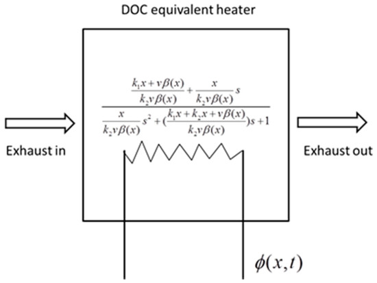
Figure 2.
The equivalent heater model of the DOC.
2.3. Relationship between the Φ and Dosing Rate of Diesel Fuel
The equations above propose a second-order linear model between the input Φ and outputs ΔTg and ΔTs. As for the relationship between the Φ and dosing rate of diesel (uinj), it is hard to reduce it, because the process from the dosing pulse width to the source term energy involves evaporation, thermolysis, mass transfer, absorption, catalytic reaction, and desorption. In this paper, the source term of input Φ is estimated by the oxygen sensor in engineering. Hence, the comparison of Φ and uinj can be directly experimentally investigated. The experimental relationship between input uinj and output Φ is shown in Figure 3. In this investigation, three different dosing rates are experimentally investigated under a 1600 r/min 50% torque condition, 2000 r/min 50% torque condition, and 2400 r/min 50% torque condition. The dosing parameters are 40 Hz, 1000 μs (Inj1); 40 Hz, 1500 μs (Inj2); and 40 Hz, 2000 μs (Inj3).
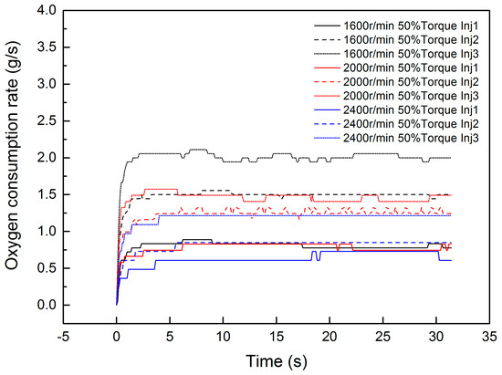
Figure 3.
The response of oxygen consumption under different conditions.
It is worth mentioning that r/min is the unit of the engine speed, which represents the revolutions per minute. The torque percentage is the ratio of the current torque to the current engine speed maximum torque. This is a general method for condition division in diesel engineering. The dosing rate is controlled by pulse width modulation (PWM). Hence, Hz is the unit of frequency, and μs is the time unit of the dosing pulse width.
The step response of uinj in the reaction model has approximate first-order characteristics. However, it costs less than 3 s to reach the peak value after dosing. As for the other conditions, the time to reach a steady state of oxygen consumption is most often less than 5 s. The statics of time are shown in Figure 4, according to hundreds of experimental groups. From the figure, about 88.2% of groups need less than 5 s to reach the steady state of oxygen consumption. Only light-load conditions, which have a lower mass flow rate, take more time to reach the steady state of oxygen consumption. As for the whole heating-up process of the DOC, most conditions need more than 60 s to reach the peak temperature in the outlet. The oxygen consumption rate is determined by the catalytic rate of C3H6, DF1, and DF2. The equation is shown in Equation (26).
where tp represents the necessary time for the oxygen rate to approximately reach steady state. From Equation (16), the energy release is shown. It consists of rs,C3H6, rs,DF1, and rs,DF2. Generally speaking, a quick approach to steadying the oxygen rate can correspondingly induce a quick approach to steadying the state of energy release (Φ). In other words, once the injection starts, the conversion of chemical energy to thermal energy inside tends to approximately steady the state very quickly. This conclusion is drawn from different simulations. Interested readers can simulate the model or refer to our Supplementary Materials. Because of the limitation of space, the simulation results are omitted here.
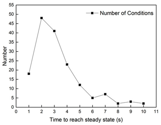
Figure 4.
The statics of time to reach a steady reaction rate.
While the connections between Φ and the dosing rate are composed of different chemical processes, a fast response relationship in the time dimension is adopted, according to the experimental result. The chemical conversion is reflected in the factor of K.
As a result, the relationship between the input uinj and output Φ is treated as a zero-order transfer function, because Φ has a very quick response under most conditions, according to experimental data. The reduced model is shown in Figure 5.
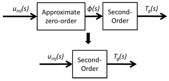
Figure 5.
Model-order reduction diagram.
The uinj in actual engineering has a different unit. For the physical process, the uinj represents the HC dosing rate. As for ECU, the uinj represents the dosing pulse width. However, the different unit of uinj can be modified by K in the transfer function. Tw and ζ remain unchanged with different units of uinj. Hence, uinj is normalized to eliminate the effect of the unit in the following section.
According to our derivation and assumption, the DOC thermodynamic model is reduced to a second-order time-varying model.
3. Experimental Section
The experimental system is composed of a diesel engine bench, HC doser, and DOC. In this system, the HC doser is mounted near the inlet of the DOC, which is 10 cm upstream of the DOC entrance. The doser is controlled by PWM. The monitor sends the controller area network (CAN) frame, which contains the PWM pulse frequency and pulse width, to the doser control unit (DCU). In the experiment, 40-Hz and 100-Hz frequencies are used. Different dosing rates are regulated by different pulse widths. The calibration results of the pulse width are shown in Table 1.

Table 1.
Dosing parameters.
The exhaust is generated by a JAC2.7L diesel engine, the performance of which is listed in Table 2. All structures of the experimental system are shown in Figure 6. In this system, the after-treatment structure only consists of the DOC and HC doser. The HC tank is used to supply the diesel fuel for dosing. The sensors mounted on the exhaust pipe are used for measuring the mass flow rate and oxygen concentration.
Table 2.
JAC 2.7L diesel parameters.
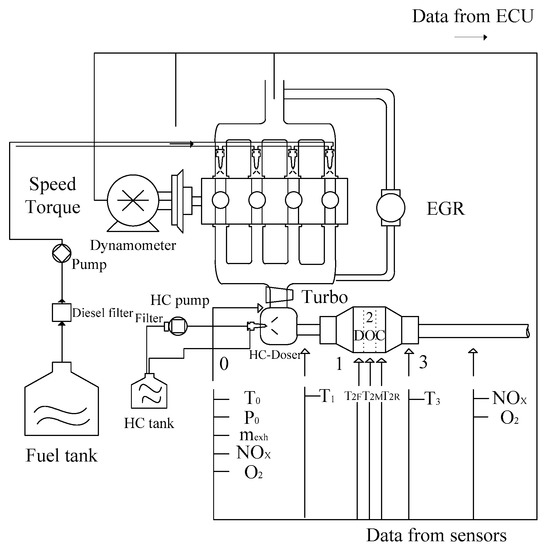
Figure 6.
Schematic of the experimental bench system.
Five K-type thermocouples were mounted inside the DOC to record the thermal behaviors. One was on the inlet of the DOC, and the other was mounted on the outlet of the DOC. Three K-type thermocouples were inserted inside the DOC. The installation diagram of the five sensors is shown in Figure 7. The diameter of the thermocouples is 1 mm, which increases the sensitivity to temperature and allowed them to be easily inserted into the flow path of the substrate, with little damage to the DOC. In Figure 7 and Figure 8, T2_in, T2_F, T2_M, T2_R, and T2_out measure the exhaust temperature at each position. Among the sensors, T2_F and T2_R have some interference from the solid phase.
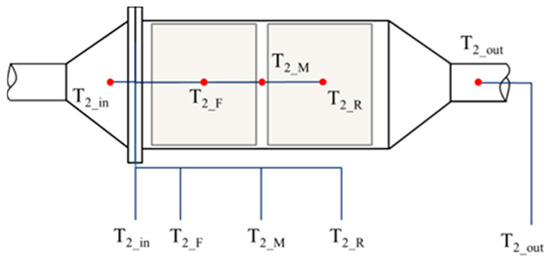
Figure 7.
Layout of the five thermocouples inside the DOC.
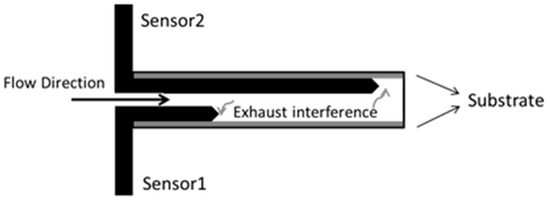
Figure 8.
Layout of the thermocouples in the axial direction.
The experiment was performed under different steady-state conditions. Under each condition, dosing started when the mass flow rate and exhaust temperature remained constant. Afterward, sensors began to record the step response to different constant dosing. The dosing ended when the recorded data reached the steady state. The parameters of the experimental conditions are shown in Table 3.
Table 3.
Parameters of the steady conditions.
4. Identification Process and Results
4.1. Identification Process
Matlab® has an app, named “system identification toolbox”, which can easily identify the model between the input data and output data. In order to investigate the experimental data, we constructed an input–output array. The variable of uinj was normalized as “1” and “0” to represent the constant dosing rate and the end of dosing. After the construction of the input–output array, “process models” was utilized.
After system identification, the identification and comparison results are shown in Figure 9. The relative error is also present in the figure. From the curve of error, the peak value was less than 0.3%. A tiny fluctuation appeared in the heating-up and cooling-down processes. The response of the oxygen reaction rate, shown in Figure 10, approximated the step signal. In order to evaluate the identification results, “accuracy”, offered by Matlab, was used for evaluation. The equation of “accuracy” is as follows:
where yi represents the experimental data at each sample time, and xi is the identification result at each time step; is the average of the identified experimental data. The accuracy of the second-order system, calculated by the identification result, was 98.2%. By comparison, the first-order system accuracy was only 81.4%. Due to the high precision and theoretical derivation, the experimental data were all identified by the second-order model. The identification results are proposed in the following section.
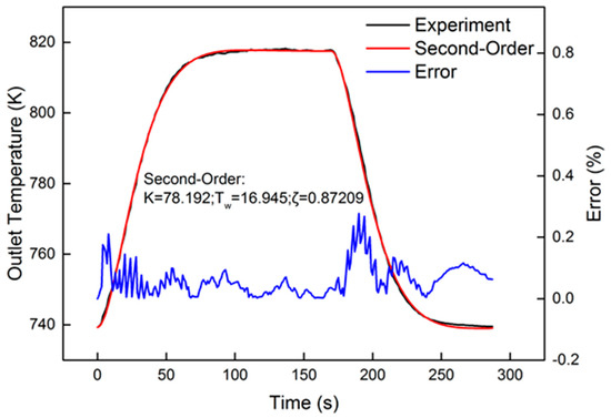
Figure 9.
Identification result of the 1600 r/min 75% torque condition, with 40 Hz, 1000 μs dosing.
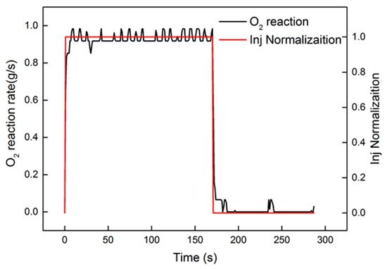
Figure 10.
Comparison of the oxygen reaction rate and injection normalization.
4.2. Identification Results
4.2.1. Identification in Axial Positions
Figure 11 shows the identification results under the 2000 r/min 75% torque condition with the 40 Hz, 2000 μs dosing rate in the axial direction. The identified parameters are also presented in the figure. Compared to the front region, the rear region had a higher Tw and higher K. The reason can be explained by Equation (25). In Equation (25), Tw and K decrease with the increase in axial position. As for ζ, the equation is a non-monotone function, the trend of which is hard to investigate in the axial direction. The relative errors are shown in Figure 12. Obviously, M_gas and R_DOC had a peak error in the dynamic cooling-down process. The error was from β, which is not a constant in actual engineering. However, the peak error was less than 0.6%. It is shown that, although β is not a constant, it did not vary much; thus, it is entirely reasonable to consider it as a constant under steady-state conditions. Under these conditions, using a second-order linear model with two poles to identify the thermodynamics of the DOC temperature will induce a high-precision order reduction. From the results, it maintained a high precision of second-order characteristics in the axial direction.
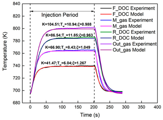
Figure 11.
Temperature comparison in different axial locations.
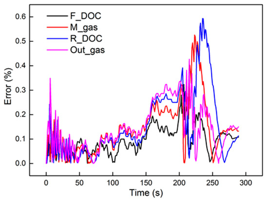
Figure 12.
The errors of the experimental data and second-order model.
4.2.2. Identification with Different Dosing Rates
In order to validate the characteristics of the second-order model with different dosing rates, an experiment was performed under the 2000 r/min 50% torque condition. Six groups of dosing rates were selected for comparison. The groups were 40 Hz, 1000 μs; 40 Hz, 1500 μs; 40 Hz, 2000 μs; 100 Hz, 1000 μs; 100 Hz, 2000 μs; and 100 Hz, 3000 μs. The experimental data were identified using the second-order linear model. The identified results are also proposed in Figure 13 for comparison. The identified parameters are shown in Table 4.
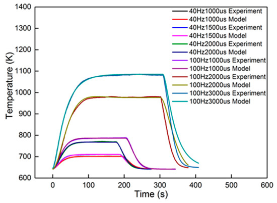
Figure 13.
The errors of the experimental data and second-order model.
Table 4.
Identification results of different dosing rates.
From the results, dosing from 40 Hz, 1000 μs to 100 Hz, 1000 μs had an accuracy higher than 94.5%. The dynamic errors of these four dosing rates are proposed in Figure 14. The peak value in the figure is less than 0.8%, proving that the second-order linear model can satisfy the dynamics of the heating-up and cooling-down processes, with different dosing rates. However, when the dosing parameters increased to 100 Hz, 2000 μs and 100 Hz, 3000 μs, the accuracy decreased to less than 85%. The dynamic errors are shown in Figure 15.
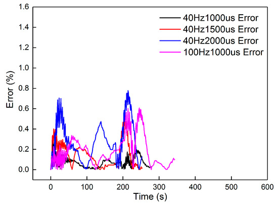
Figure 14.
The errors of the four groups.
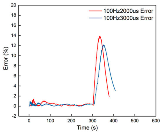
Figure 15.
The errors of the 100 Hz, 2000 μs and 100 Hz, 3000 μs groups.
The peak error from the figure was 14%, which appeared in the cooling-down process. From the curves in Figure 14, it is also obvious that the corresponding curves were divided into two parts into 100 Hz, 2000 μs and 100 Hz, 3000 μs, when in the cooling-down process. From the experimental results, the reduced model had a slower decrement compared to the experimental curve. The explanation is that the parameters of the cooling process were different from the heating-up process, when the dosing rate was considerable. Hence, the cooling-down process should use other groups of second-order parameters. After identification, the new results are shown in Table 5. New curves are shown in Figure 16. The dynamic errors are shown in Figure 17. The peak error was reduced to 1.4% using the divided second-order parameters.
Table 5.
New identification results of the 100 Hz, 2000 μs and 100 Hz, 3000 μs groups in the cooling-down process.
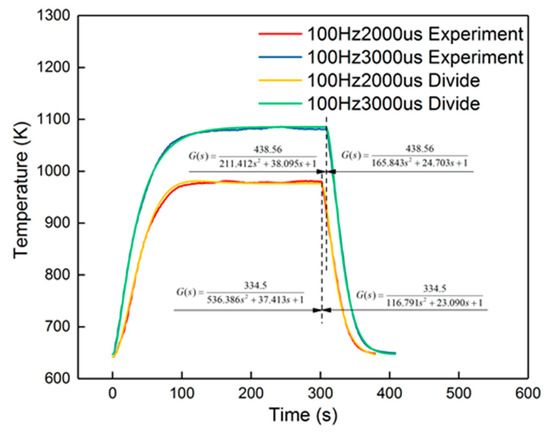
Figure 16.
Divided identification results of the 100 Hz, 2000 μs and 100 Hz, 3000 μs groups.
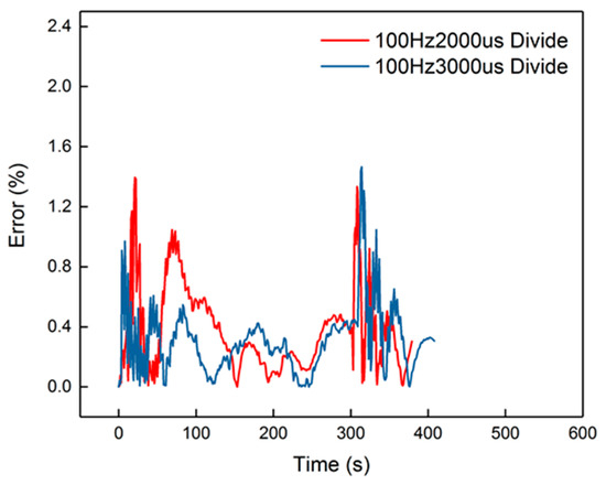
Figure 17.
Errors of the divided identification.
As a result, second-order identification with different dosing rates has high precision. The higher error that appears under a higher temperature condition can be eliminated using divided identification. After the division of the heating-up identification and cooling-down identification, the curves fit well with the second-order model.
Considering the dosing rate effect, the real K is proposed in Figure 18. The equation between K and real K is as follows:
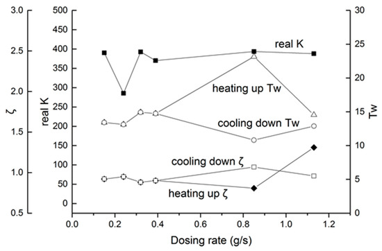
Figure 18.
Second-order parameters, with different dosing rates.
From Figure 18, for most parameters in the K range, from 370 to 390, only the 40 Hz, 1500 μs group had a large deviation. As for Tw and ζ, the parameters had a little change from 0.15 g/s to 0.39 g/s. When the dosing rate was higher than 0.4 g/s, deviations in Tw and ζ appeared. As a conclusion, the increment of the dosing rate induces some irregularity, which needs online identification or more intensive calibration to determine the actual parameters.
4.2.3. Identification under Different Steady Conditions
In order to validate the second-order characteristics under different conditions, the identification results under different conditions with the 40 Hz, 2000 μs dosing rate are shown in Table 6. The outlet temperature was used for identification.
Table 6.
Second-order identification results under different conditions.
The identification was only performed in the heating-up process, after the start of dosing. The accuracies shown in the table are higher than 94%. This proves that the thermodynamics of the DOC have second-order characteristics under most conditions. If the conditions change, and the dosing rate varies in the actual thermal management of the diesel after-treatment system, the DOC thermodynamics can be treated as a second-order time-varying system.
Considering the change in conditions, it is meaningful to investigate the changing rules of K, Tw, and ζ. The value of K under a low-speed and light-load condition is larger than that under other conditions. When the speed and torque increase, the values of K gradually decrease. As for Tw, the decrement is significant when the speed increases. This can be explained by Equation (25). The value of Tw has a proportional relationship with . Hence, a higher mass flow rate of the exhaust induces a lower Tw.
As for ζ, a lower value appears under low-speed and high-load conditions. Under these conditions, the temperature has less resistance than when heating up. Under other conditions, the changing rules of ζ are not obvious, but the range is from 1.0–1.5. The real value should be identified online or calibrated by experiment.
To sum up, higher-speed and higher-load conditions induce a lower K and lower Tw. The conditions with a lower speed and higher load induce a lower ζ. When the conditions are varying within a certain scope, the three parameters correspondingly vary within a certain numerical range. Online identification or intensive calibration is required to clarify the determination of the real values.
5. Conclusions
The results of this study show that the thermodynamics of the DOC can be reduced to a second-order time-varying system. Identification was performed in different axial positions inside the DOC, with different dosing rates and under different engine conditions. The conclusions are as follows:
- (1)
- The experimental data have a high precision in fitting with the second-order characteristics.
- (2)
- When the axial location is given, constant dosing under steady conditions can reduce the thermodynamics of the DOC to a second-order transfer function, with constant parameters, both in the theoretical derivation and in the experimental result.
- (3)
- In the axial direction, parameter K is higher in the rear and outlet regions than in the front region of the DOC. Tw also has the same performance as K. However, ζ has less regularity in axial distribution.
- (4)
- With a differing dosing rate, the regularity of K, Tw, and ζ is not obvious.
- (5)
- Under different steady conditions, higher-speed and higher-load conditions induce a lower K and lower Tw. A lower speed and higher load induce a lower ζ.
- (6)
- The range of Tw is from 6–32, and the range of ζ is from 0.75–1.5 when the engine conditions range from 1200 r/min 50% torque to 2800 r/min 100% torque.
As a result, the thermodynamics of the DOC with HC dosing can be reduced to a second-order time-varying model, as a theoretical basis for other researchers and engineers.
Supplementary Materials
The following are available online at https://www.mdpi.com/2073-4344/9/4/369/s1, Figure (a)(b)(c)(d)(e): Step response of HC-dosing under different steady conditions.
Author Contributions
Individual contributions are as follows: F.W., B.Z. and D.Y.; methodology, B.Z.; software, B.Z.; validation, B.Z.; formal analysis, B.Z.; investigation, B.Z.; resources, F.W., Y.Y.; data curation, B.Z; writing-original draft preparation, B.Z.; writing-review and editing, B.Z., D.Y.; visualization, B.Z.; supervision, F.W. and D.Y.; project administration, F.W. and D.Y.; funding acquisition, F.W., D.Y. and Y.Y.
Funding
This research was funded by National Key R&D Program of China, grant number 2017YFC0211103; as well as by CN-6 After-treatment technologies of Diesel engine R&D Program, grant number K17-508106-029.
Conflicts of Interest
The authors declare no conflict of interest. The funders had no role in design of the study; in the collection, analyses, or interpretation of data; in the writing of the manuscript, or in the decision to publish the results.
References
- Zheng, G.; Kotrba, A.; Golin, M.; Gardner, T.; Wang, A. Overview of Large Diesel Engine Aftertreatment System Development. In SAE Technical Paper 2012-01-1960, Proceedings of the Commercial Vehicle Engineering Congress SAE, Chicago, IL, USA, 2–3 October 2012; SAE International: Chicago, IL, USA, 2012. [Google Scholar]
- Park, D.S.; Kim, J.U.; Kim, E.S. A burner-type trap for particulate matter from a diesel engine. Combust. Flame 1998, 114, 585–590. [Google Scholar] [CrossRef]
- Hasan, M.; Venkata, R.L.; Johnson, J.H.; Bagley, S.T. An Experimental and Modeling Study of a Diesel Oxidation Catalyst and a Catalyzed Diesel Particulate Filter using a 1-D 2-Layer Model. In SAE Technical Paper 2006-01-0466, Proceedings of the SAE 2006 World Congress & Exhibition, Detroit, MI, USA, April 9 2006; SAE International: Detroit, MI, USA, 2006. [Google Scholar]
- Huang, J.; Huang, H.; Liu, L.; Jiang, H. Revisit the effect of manganese oxidation state on activity in low-temperature NO-SCR. Mol. Catal. 2018, 446, 49–57. [Google Scholar] [CrossRef]
- Cozzolini, A.; Mulone, V.; Abeyratne, P.; Littera, D.; Gautam, M. Advanced Modeling of Diesel Particulate Filters to Predict Soot Accumulation and Pressure Drop. In SAE Technical Paper 2011-24-0187, Proceedings of the 10th International Conference on Engines & Vehicles, Naples, Italy, 11–15 September 2011; SAE International: Morgantown, WA, USA, 2011. [Google Scholar]
- Kim, Y.W.; Van Nieuwstadt, M.; Stewart, G.; Pekar, J. Model Predictive Control of DOC Temperature during DPF Regeneration. In SAE Technical Paper 2014-01-1165, Proceedings of the SAE 2014 World Congress & Exhibition, Detroit, MI, United States, 8–10 April 2014; SAE International: Detroit, MI, USA, 2014. [Google Scholar]
- Hein, E.; Kotrba, A.; Inclan, T.; Bright, A. Secondary Fuel Injection Characterization of a Diesel Vaporizer for Active DPF Regeneration. SAE Int. J. Engines 2014, 7, 1228–1234. [Google Scholar] [CrossRef]
- Harned, J.L. Analytical Evaluation of a Catalytic Converter System. In SAE Technical Paper 720520, 1972, Proceedings fo the National Automobile Engineering Meeting, Detroit, MI, USA, 1 February, 1972; SAE International: Detroit, MI, USA, 1972. [Google Scholar]
- Kuo, J.; Morgan, C.; Lassen, H. Mathematical Modeling of CO and HC Catalytic Converter Systems. In SAE Technical Paper 710289, Proceedings of the 1971 Automotive Engineering Congress and Exposition, Detroit, MI, United States, 1 February, 1971; SAE International: Detroit, MI, USA, 1971. [Google Scholar]
- Vardi, J.; Biller, W.F. Thermal behavior of exhaust gas catalytic convertor. Ind. Eng. Chem. Process Des. Dev. 1968, 7, 83–90. [Google Scholar] [CrossRef]
- Oh, S.H.; Cavendish, J.C. Transients of monolithic catalytic converters. Response to step changes in feedstream temperature as related to controlling automobile emissions. Ind. Eng. Chem. Prod. Res. Dev. 1982, 21, 29–37. [Google Scholar] [CrossRef]
- Groppi, G.; Belloli, A.; Tronconi, E.; Forzatti, P. A comparison of lumped and distributed models of monolith catalytic combustors. Chem. Eng. Sci. 1995, 50, 2705–2715. [Google Scholar] [CrossRef]
- Voltz, S.E.; Morgan, C.R.; Liederman, D.; Jacob, S.M. Kinetic study of carbon monoxide and propylene oxidation on platinum catalysts. Ind. Eng. Chem. Prod. Res. Dev. 1973, 12, 294–301. [Google Scholar] [CrossRef]
- Kryl, D.; Kočí, P.; Kubíček, M.; Marek, M.; Maunula, T.; Härkönen, M. Catalytic converters for automobile diesel engines with adsorption of hydrocarbons on zeolites. Ind. Eng. Chem. Res. 2005, 44, 9524–9534. [Google Scholar] [CrossRef]
- Sampara, C.S.; Bissett, E.J.; Chmielewski, M.; Assanis, D. Global kinetics for platinum diesel oxidation catalysts. Ind. Eng. Chem. Res. 2007, 46, 7993–8003. [Google Scholar] [CrossRef]
- Sampara, C.S.; Bissett, E.J.; Chmielewski, M. Global kinetics for a commercial diesel oxidation catalyst with two exhaust hydrocarbons. Ind. Eng. Chem. Res. 2008, 47, 311–322. [Google Scholar] [CrossRef]
- Depcik, C.; Assanis, D. One-dimensional automotive catalyst modeling. Prog. Engery Combust. Sci. 2005, 31, 308–369. [Google Scholar] [CrossRef]
- Hazlett, M.J.; Moses-Debusk, M.; Parks, I.I.; Allard, L.F.; Epling, W.S. Kinetic and mechanistic study of bimetallic Pt-Pd/Al 2 O 3 catalysts for CO and C 3 H 6 oxidation. Appl. Catal. B Environ. 2017, 202, 404–417. [Google Scholar] [CrossRef]
- Olsson, L.; Andersson, B. Kinetic modelling in automotive catalysis. Top. Catal. 2004, 28, 89–98. [Google Scholar] [CrossRef]
- Oluku, I.; Khan, F.; Idem, R.; Ibrahim, H. Mechanistic kinetics and reactor modelling of hydrogen production from the partial oxidation of diesel over a quartenary metal oxide catalyst. Mol. Catal. 2018, 451, 255–265. [Google Scholar] [CrossRef]
- Peng, P.Y.; Harold, M.P.; Luss, D. Sustained concentration and temperature oscillations in a diesel oxidation catalyst. Chem. Eng. J. 2018, 336, 531–543. [Google Scholar] [CrossRef]
- Lepreux, O.; Creff, Y.; Petit, N. Model-based temperature control of a diesel oxidation catalyst. J. Process Control 2012, 22, 41–50. [Google Scholar] [CrossRef]
- Bencherif, K.; Benaicha, F.; Sadaï, S.; Sorine, M. Diesel Particulate Filter Thermal Management Using Model-Based Design. In SAE Technical Paper 2009-01-1082, Proceedings of the SAE World Congress & Exhibition, Detroit, MI, United States, 20–23 April, 2009; SAE International: Detroit, MI, USA, 2009. [Google Scholar]
- Chen, P.; Wang, J. Control-oriented model for integrated diesel engine and aftertreatment systems thermal management. Control Eng. Pract. 2014, 22, 81–93. [Google Scholar] [CrossRef]
- Donkers, M.C.F.; Van Schijndel, J.; Heemels, W.P.M.H.; Willems, F.P.T. Optimal control for integrated emission management in diesel engines. Control Eng. Pract. 2017, 61, 206–216. [Google Scholar] [CrossRef][Green Version]
- Ning, J.; Yan, F. Composite Control of DOC-out Temperature for DPF regeneration. IFAC PapersOnLine 2016, 49, 20–27. [Google Scholar] [CrossRef]


© 2019 by the authors. Licensee MDPI, Basel, Switzerland. This article is an open access article distributed under the terms and conditions of the Creative Commons Attribution (CC BY) license (http://creativecommons.org/licenses/by/4.0/).