Abstract
The modeling and simulation of the catalytic dehydrogenation process of cyclohexanol in a fixed-bed catalytic reactor is presented, leading to finding the relationship between the effectiveness factor, the Thiele modulus, and the Weisz–Prater modulus of the catalyst particles with respect to their axial and radial position, for which the external conditions of concentration and temperature around each particle were previously obtained by applying the material and energy balances in the catalyst bed considering a two-dimensional pseudo-homogeneous model with radial diffusion. Subsequently, the material balances are established in terms of the molar flux density and conversion, the energy balance in terms of the heat flux density, Fick’s law, Fourier’s law, and the differential form of the effectiveness factor non-isothermal for each particle chosen based on the proposed meshing. The Thiele modulus calculated for most of the points is between 0.8 and 0.25, with a tendency towards the lower limit, and the theoretical values established as the limit for the Thiele modulus fluctuate between . Therefore, the effectiveness factor analyzed is between 1 and ; this indicates that both the reaction speed as well as the diffusion speed within the particle have an influence on the intraparticle process, which is confirmed by the calculation of the Weisz–Prater modulus whose values are not 1 nor 1. The results obtained are subjected to a statistical test leading to analyzing whether there are significant differences both in the Thiele modulus, as well as in the effectiveness factor with respect to the radius and length of the reactor. It has been determined that there are no significant differences between the effectiveness factor with respect to the radius of the reactor; however, according to the analysis of variance, there are significant differences in the effectiveness factor with respect to length and, likewise, there are significant differences in the Thiele modulus and the Weisz–Prater modulus with respect to radius and length.
1. Introduction
The dehydrogenation of cyclohexanol to cyclohexanone on a zinc oxide catalyst mainly produces cyclohexanone with a selectivity greater than 93%, its basic reaction is . In the literature, it is pointed out that dehydration (aldol condensation) and dimerization should be taken into account as secondary reactions [1]. The technical sheet mentions that cyclohexanone is mainly used in the manufacture of nylon and as an adhesive in sealing PVC objects, it is also used as a solvent for lacquers, resins, polymers, adhesives, pigments, and in other applications; cyclohexanone can be present together with other solvents, especially in adhesives and lacquers. This information is complemented by the work of Romero et al. [2] and Lorenzo et al. [3] who point out that cyclohexanone is an important intermediate in the chemical industry for the manufacture of caprolactam and adipic acid, which is used in the production of polyamide fiber in nylon textiles. Cyclohexanone is also an important intermediate in the synthesis of pharmaceuticals and fine chemicals.
The dehydrogenation of cyclohexanol to obtain cyclohexanone is carried out using a series of catalysts that allows in some cases to improve selectivity and in other cases to decrease the rate of deactivation with adsorption of one or more reaction components. In this sense, there are kinetic expressions developed by Morita et al. [4] based on a Cu-Zn catalyst, Athappan et al. [5] based on the NiO/Al2O3 catalyst, Orizarsky et al. [6] based on a copper catalyst, Zhang et al. [7] based on the Cu-Co/MgO catalyst. Two specific models for the dehydrogenation of cyclohexanol based on the ZnO catalyst have been reported according to Gut and Jaeger [1], who propose a second-order kinetic model for the adsorption of alcohol, ketone, and hydrogen. Recently, Patil et al. [8] reported a study on the effect of precipitating agents on the activity of coprecipitated Cu-MgO catalysts towards selective furfural hydrogenation and cyclohexanol dehydrogenation reactions. At the same time, Joseph et al. [9] reported on the energy-efficient synthesis of cyclohexanone with high selectivity, through the photocatalytic dehydrogenation of cyclohexanol using the green and robust ternary nanohybrid photocatalyst. Unlike the authors cited, García-Ochoa et al. [10] propose the kinetic model, which takes into consideration the data from the catalyst, the process, and the geometric conditions of the reactor as necessary to carry out the modeling, both in the reactor and in the particles.
The adsorption equilibrium constant based on the dehydrogenation reaction of cyclohexanol using the zinc oxide catalyst was reported by Stull et al. [11] and Cubberly and Mueller [12]. In their work, they point out that the global catalytic dehydrogenation reaction of cyclohexanol in a pseudo-homogeneous fixed-bed tubular reactor is highly endothermic and its conversion is limited by equilibrium.
The reaction rate corresponding to the dehydrogenation of cyclohexanol using zinc oxide as a catalyst has been proposed by García-Ochoa et al. [10], whose expression is shown in Equation (1), and is given in terms of the partial pressure of cyclohexanol (), and the reaction temperature (T):
where the constants have the values of , , and [10].
The modeling of the cyclohexanol dehydrogenation was initially proposed by García-Ochoa et al. [10], who considered a pseudo-homogeneous, non-adiabatic, two-dimensional fixed-bed tubular reactor, for which they proposed mass and energy balances, with the diffusion of matter and energy in the radial direction. They used the orthogonal placement method to obtain the conversion and temperature profiles.
In 2018, Carrasco [13], using the data of reaction kinetics, process, and reactor geometry proposed by García-Ochoa et al. [10], developed the modeling of the dehydrogenation of cyclohexanol, considering a tubular reactor with radial and axial diffusion, pseudo-homogeneous and non-adiabatic, which led to the formulation of two partial differential equations that were solved by the method of implicit finite differences. When compared with the results of García-Ochoa et al. [10], similarities were observed in the results, which implies little influence of axial diffusion on the final result. In this sense, he proposed the non-adiabatic two-dimensional pseudo-homogeneous model with radial diffusion, whose solution by the Lines method was much more feasible to implement.
Regarding the process inside the catalyst, Davis and Davis [14], point out that to most efficiently use a catalyst in a commercial operation, the reaction rate must often be adjusted to be approximately the same order of magnitude as the diffusion rates. If a catalyst particle in an industrial reactor was operating at an extremely low rotational frequency, the diffusive transportation of chemicals to and from the catalyst surface would have no effect on the measured velocities. Likewise, if a catalyst particle was operating under conditions that normally give extremely high rotational frequency, the observed overall reaction rate is reduced by inadequate transportation of reactants to the catalyst surface. The balance between the reaction rate and the transportation phenomena is often considered the most efficient means of operating a catalytic reaction.
The Thiele modulus and the effectiveness factor are important parameters to estimate the effectiveness of a biochemical transformation process, Azimi and Azimi [15], or chemical, Fogler [16]. For this last case, since the reactions are normally carried out under non-isothermal conditions, it is also required to know the Weisz–Prater modulus. The effects of heat transfer in a gas–solid reaction were studied by Kimura et al. [17], who applied the simplified method for the estimation of the effectiveness factor, with the use of the Thiele modulus, the Prater number, and the Arrhenius number. Their results are represented graphically for highly exothermic reactions in multiple cases.
According to De Silva et al. [18] and Iordanidis [19], the Thiele modulus is defined as the ratio between the rate of reaction and the rate of gas diffusion within the catalyst particle. The highest diffusion rate occurs when the pore size is large; therefore, the larger the pore size, the Thiele modulus will be smaller since the relationship with the diffusion coefficient is inverse.
The effectiveness factor (η) measures the slowing down of the reaction rate caused by the resistance to diffusion within the particle [16,20], which is obtained from the quotient between the actual mean reaction rate inside the particle and the reaction rate under surface conditions. Zhu et al. [21] analyzed the influence of the spatially distributed pore size and the porosity on the reactive and diffusion characteristics within the porous catalyst particle.
There are a number of methods for estimating the effectiveness factor. According to the work of Sun et al. [22], the Adomian decomposition method is used to study the problem of diffusion and reaction in catalyst pellets. For their study, they considered solving the nonlinear diffusion and reaction model, which allows for obtaining approximate solutions. The variation of the reagent concentration in the catalyst pellets and the efficiency factors are determined for second, middle, and first-order reactions. The approximate analytical solutions obtained are compared with solutions obtained with a finite difference numerical method.
The best-known method for estimating the effectiveness factor is the so-called general method that considers the material balances of each component, Fick’s law for each component, the energy balance, Fourier’s law, and the integral or differential method for the calculation of the effectiveness factor. This set of equations is solved using numerical methods; specifically, the implicit finite difference method, Cutlip and Shacham [23], with which the profiles of molar flux density for each component are obtained using the concentration of each component, heat flux density, temperature, and Thiele modulus, as well as the effectiveness factor and consequently the Weisz–Prater modulus, for the cyclohexanol dehydrogenation process using the zinc oxide catalyst in spheres.
The development of this work is important, not only from the academic point of view but also from the point of view of industrial application since the determination of the effectiveness factor profiles together with the concentration and temperature profiles allows us to visualize the zones of greater and less effectiveness of the reactor. This knowledge is important to make necessary decisions such as modification of parameters, inlet temperature, partial pressure of cyclohexanol at the reactor inlet, particle size, reactor diameter, reactor length, heating temperature, and the flow of feeding, among others, in order to increase the conversion and selectivity towards the formation of cyclohexanone, which means, it is possible to optimize this catalytic process.
Consequently, the objective of the work is to obtain the radial and axial profiles of conversion and temperature in the catalytic bed, that is, the external conditions on the catalyst surface. With this knowledge, specific points (r, z) of the reactor are chosen, which correspond to the location of the catalyst particle, which allows obtaining for each selected particle both their respective conversion profiles, as well as the temperature inside the particle. Allowing in return to obtain the Thiele modulus, the effectiveness factor, and the Weisz–Prater modulus for each particle, with which it is possible to establish the profiles of these parameters as a function of radius and length. Likewise, the statistical analysis of the significance of the Thiele modulus, the effectiveness factor, and the Weisz–Prater modulus with respect to the radius and length of the reactor is made.
2. Results
2.1. Regarding the Gas Phase (External Conditions to the Catalyst Particles)
Based on the data in Table 1, the length of the reactor used is 300 cm and its radius is 5 cm. This last value has been subdivided into 10 placement points by considering the phenomenon of radial diffusion. The calculation program called reactor.pol, developed using the Polymath software, allows solving Equations (24) and (25), as well as the differential equations derived from the generic Equations (26) and (27), making a total of 22 ordinary differential equations which are solved considering the data presented in Table 1.

Table 1.
Data of the cyclohexanol dehydrogenation process.
After the execution of the program, the data of Table A1 and Table A2 were obtained, conveniently reduced due to their length. With these data, the graphs of Figure 1 and Figure 2 were obtained. From the indicated graphs, it can be seen that the length of 3 m referring to the reactor is oversized since at an approximate length of 2 m the maximum conversion of cyclohexanol is reached, whose value is 1.
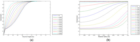
Figure 1.
Graphical representation of the conversion profile of cyclohexanol to cyclohexanone: (a) conversion profile of cyclohexanol as a function of length for each placement point along the radius of the reactor, and (b) conversion profile of cyclohexane as a function of radius for each position longitudinal. Obtained from the data in Table A1.
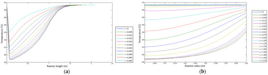
Figure 2.
Graphical representation of the reaction temperature profile of the conversion of cyclohexanol to cyclohexanone: (a) temperature profile as a function of length for each placement point along the radius of the reactor, and (b) temperature profile as a function of radius for each longitudinal position. Source: obtained from the data in Table A2.
2.2. Regarding the Solid Phase (Conditions inside the Catalyst Particle)
Based on the results obtained with the program reactor.pol (Table A1 and Table A2) and with the data in Table 1, the program particula.pol was developed, which allows obtaining for each particle located at a specific point , by simultaneous resolution of Equations (51)–(55), the following data set:
- Molar flux density profile of each component.
- Heat flux density profile.
- Concentration profile of each component.
- Conversion profile of cyclohexanol.
- Temperature profile.
- Thiele modulus profile.
- Effectiveness factor profile.
The values of the last two profiles are observed in Table A3 and Table A4. The distribution of the effectiveness factor of each particle in the catalytic bed is observed in Figure 3a–c, and the dependence of the Thiele modulus in terms of length and radius is observed in Figure 3d.
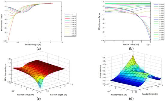
Figure 3.
Representation of the profiles inside the particle in the cyclohexanol dehydrogenation process: (a) profile of the effectiveness factor as a function of the length for each placement point along the radius of the reactor, (b) profile of the effectiveness factor as a function of to the radius of the reactor for each length, (c) profile of the effectiveness factor as a function of the length and radius of the reactor (obtained from Table A4), and (d) profile of the Thiele modulus as a function of the radius and length (obtained from Table A3).
The conversion profiles (Figure 1a,b) and temperature in the bed (Figure 2a,b) are external conditions of the catalyst particles and are a function of radius and length, they have a nonlinear relationship. These external conditions are used to obtain the Thiele modulus for each particle, which is associated with the square root of the reaction rate and the diffusion rate, Equation (57). The effectiveness factor depends on the external conversion conditions, temperature, internal mass, and heat transfer processes (diffusion, adsorption, reaction, desorption, etc.). The Weisz modulus has a quadratic relationship against the product of the effectiveness factor and the Thiele modulus, Equation (59). Consequently, by associating all these criteria of the external conditions in the bed and the internal processes within each particle, it is established that said relationships have a dependence on the effectiveness factor and the Thiele modulus as a function of the radius (Figure 4a), dependence between the effectiveness factor and the Thiele modulus as a function of the length (Figure 4b), the relationship of the Weisz–Prater modulus versus the radius and length of the reactor (Figure 4c), and the dependence of the Weisz–Prater modulus and the effectiveness factor (Figure 4d), have a markedly nonlinear dependence.
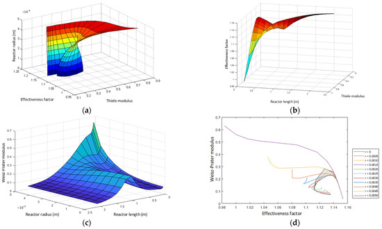
Figure 4.
Graphical representation of the profiles inside the catalyst particle: (a) graphical representation of the effectiveness factor as a function of the Thiele modulus and the radius of the reactor, (b) graphical representation of the effectiveness factor as a function of the Thiele modulus and the length of the reactor, (c) graphical representation of the Weisz–Prater modulus factor as a function of the radius and length of the reactor, and (d) graphical representation of the Weisz–Prater modulus as a function of the effectiveness factor (obtained from Table A3 and Table A4).
2.3. Variance Analysis
The variance analysis of the effectiveness factor data and the Thiele modulus was carried out to see if there is a significant dependence of these parameters on the radius and length of the reactor.
3. Discussion
The dehydrogenation reaction of cyclohexanol presents two marked stages. In the first stage, approximately 10 cm from the entry point, there is a marked drop in temperature whose maximum difference is about 74 °C, due to the endothermicity of the reaction; in a second moment, an increase in temperature is observed (see Figure 2a), which also generates an increase in conversion (see Figure 1a) differentiated for each radio. The highest temperature is close to the tube wall and consequently also the highest conversion. As the length is advanced, the temperature and conversion continue to increase. However, the differences of both parameters with respect to the radius decrease considerably, obtaining a conversion equal to the unit at two meters of tube length for all radii, because the reaction reached its completion (see Figure 1b and Figure 2b).
Figure 3a,b show that the effectiveness factor depends on both the radius and the length of the reactor. The value of the effectiveness factor has the lowest value just where the drop in temperature occurs, so its values increase as the length of the reactor increases, reaching a value slightly higher than unity. However, in non-isothermal reactions, such as dehydrogenation, it is possible to obtain these values greater than unity. Figure 3c allows better visualization of the dependence of the effectiveness factor as a function of the length and radius of the reactor. Figure 3d represents the dependence of the Thiele modulus on the radius and length of the reactor, in which it can be seen that at 10 cm of reactor length, it takes the highest value (where the temperature is lowest). This would indicate that the rate of reaction on the surface is greater than the rate of diffusion.
According to Levenspiel [20], it can be indicated as a general rule for any type of geometry, that if h there is strong internal diffusional control, and the effectiveness factor can be approximated to . Instead, if internal resistances to mass transport are negligible, then . In the range the process undergoes mixed control, both the reaction rate and the diffusion rate; so both mechanisms control the process. In this case, the Thiele modulus values vary from values lower than 0.4 where diffusional effects are negligible, to higher values below 4, so in this case both the diffusional effects and the reaction rate control the reaction rate process. These processes occur at various points in the reactor.
Figure 4a,b show the dependence of the effectiveness factor on the Thiele modulus and the radius and length of the reactor. In general, it can be mentioned that at 10 cm in length, the inflection points of the effectiveness factor occur since this depends on the Thiele modulus, and this in turn depends on the temperature. Figure 4c shows a trend similar to Figure 3d because both are related by .
According to Fogler [16], the criterion to apply the controlling stage consists in determining the Weisz–Prater modulus; therefore, if there are no diffusion limitations and therefore there is no concentration gradient within the granule. While if then internal diffusion severely limits the reaction. Due to the fact that in this case, both extremes are not available, it can be affirmed that in this dehydrogenation process, both diffusion and the chemical reaction influence the process (see Figure 4c,d).
From the analysis of variance for the factor of effectiveness vs. radius, with a value p = 0.138 > 0.05, it is stated that there are no significant differences between the values of the effectiveness factor with respect to the radius (see Table 2). Figure 5 shows a progressive increase in the variation of the effectiveness factor with respect to the radius. However, the average value of this factor presents a decreasing distribution of r = 0 to r = R.
Table 2.
Analysis of variance of the effectiveness factor versus the reactor radius.
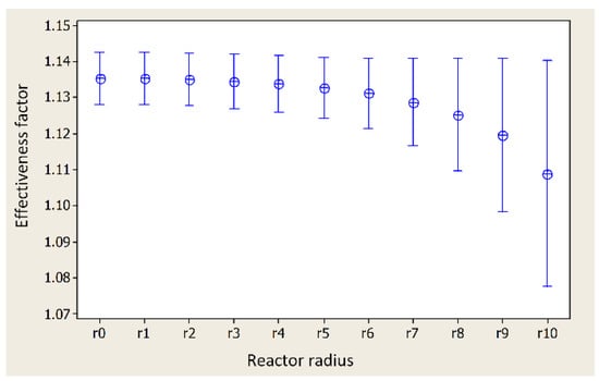
Figure 5.
Analysis of variance of the effectiveness factor vs. reactor radius (obtained from Table A4). Interval plot 95% CI for the mean.
From the analysis of variance for the effectiveness-length factor, with a value p = 0.000 < 0.05, it is stated that there are significant differences between the values of the effectiveness factor with respect to length (see Table 3). In Figure 6, the effectiveness factor presents a greater range of variability in the points close to the entrance of the reactor. For values greater than 1 m z = z9, said variability decreases significantly until it becomes practically zero for high values of reactor length. The mean value has an increasing nonlinear distribution from a value close to 1 at the reactor inlet to a value of 1.15 near the reactor outlet.
Table 3.
Analysis of variance of the effectiveness factor versus the length reactor.
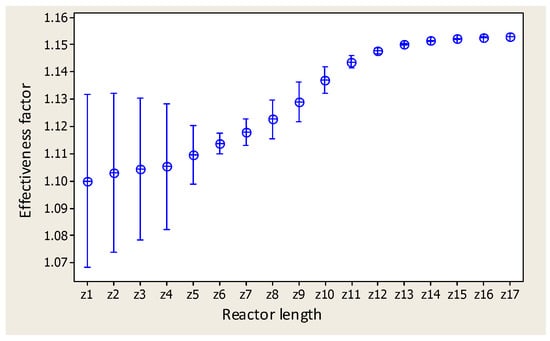
Figure 6.
Analysis of variance of the effectiveness factor vs. length reactor (obtained from Table A4). Interval plot 95% CI for the mean.
From the analysis of variance for the Thiele modulus vs. radius, with a value p = 0.001 < 0.05, it is stated that there are significant differences between the values of the Thiele modulus with respect to the radius (see Table 4). Figure 7 shows that the Thiele modulus variation ranges are constant at each radius, except near the wall where this variation increases more. Likewise, the mean value has an increasing distribution with respect to the radius from a value close to 0.3 at r = r0 to a value close to 0.45 close to r = r10.
Table 4.
Analysis of variance of the Thiele modulus versus the reactor radius.
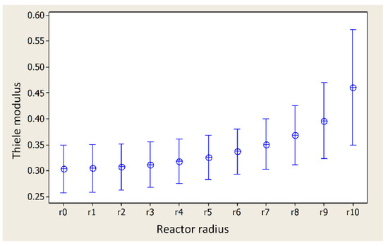
Figure 7.
Thiele modulus vs. reactor radius (obtained from Table A4). Interval plot 95% CI for the mean.
From the analysis of variance for the Thiele modulus vs. length, with a value p = 0.000 < 0.05 (see Table 5), it is stated that there are significant differences in the Thiele modulus with respect to the length of the reactor as observed in Figure 8, where the mean value distribution curve presents two stretches: The first stretch is from the reactor entry point to about 1 m, where the variation is greater at the entrance of the reactor and decreases rapidly until the indicated value of one meter. The second section has a less marked decreasing variability starting at z = 1 until the exit to the reactor.
Table 5.
Analysis of variance of the Thiele modulus versus the length reactor.
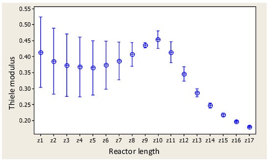
Figure 8.
Thiele modulus vs. length reactor (obtained from Table A4). Interval plot 95% CI for the mean.
For a confidence level of 95%, there are significant differences in the values of the Weisz–Prater modulus with respect to the radius (see Table 6 and Figure 9). The Weisz–Prater modulus involves the Thiele modulus and the effectiveness factor. According to the analysis regarding the variation of the effectiveness factor vs. radius, it is not significant (see Figure 5). However, with respect to the Thiele modulus, it is significant (see Figure 7). The Weisz–Prater modulus indicates that there are significant differences in said variation.
Table 6.
Analysis of variance of the Weisz–Prater modulus versus the reactor radius.
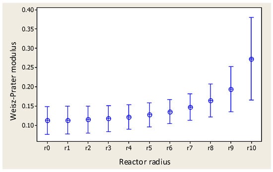
Figure 9.
Weisz–Prater modulus vs. reactor radius (obtained from Table A4). Interval plot 95% CI for the mean.
For a confidence level of 95%, there are significant differences in the values of the Weisz–Prater modulus with respect to length (see Table 7 and Figure 10). This is consistent with the significant differences found for the effectiveness factor and the Thiele modulus with respect to the length of the reactor.
Table 7.
Analysis of variance of the Weisz–Prater modulus versus the reactor longitude.
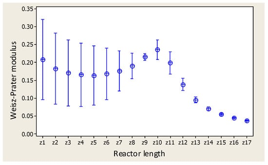
Figure 10.
Weisz–Prater modulus vs. length reactor (obtained from Table A4). Interval plot 95% CI for the mean.
4. Methods
The present work has two stages: In the first stage, the material balance is considered in terms of conversion, the energy balance, and it is solved with the help of software, obtaining the respective conversion and temperature profiles. In the second stage, modeling is carried out on the catalyst particle, setting out the material balances for each of the components of the dehydrogenation reaction, and obtaining the conversion and temperature data inside the catalyst pellet with which the effectiveness factor profiles are obtained. The reaction shows the cyclohexanol dehydrogenation process giving cyclohexanone and hydrogen as products, in the catalytic bed considered as a two-dimensional pseudo-homogeneous process.
Figure 11 shows the scheme of the catalytic bed that allows obtaining the external conversion conditions and temperature referred to the catalyst particle, with whose data the conversion profiles are obtained in the particle under non-isothermal conditions.
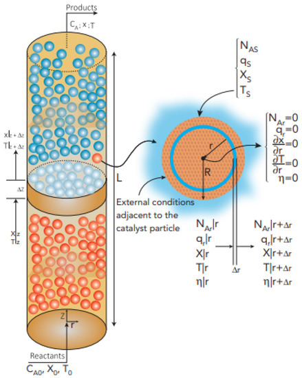
Figure 11.
Diagram of the catalytic dehydrogenation process of cyclohexanol [13].
Material and energy balances are established for a cylindrical geometry fixed-bed reactor considering the two-dimensional model with radial diffusion, according to García-Ochoa et al. [10]. The mass balance equation (subscript A = cyclohexanol, B = cyclohexanone, and C = hydrogen) in terms of concentration and temperature is given by:
The energy balance equation in terms of temperature and concentration is given by:
Equations (2) and (3) turn out to be two partial differential equations coupled by concentration and temperature. An appropriate solution method is the so-called Lines method, which consists of transforming the partial differential equations into a system of ordinary differential equations, by partial discretization of the terms that are functions of the radius. In this way, the resulting ODE system has z as an independent variable, becoming an initial value problem, which is solved by explicit methods.
From the Equation (2):
The mass transfer Peclet number is given by:
Putting Equation (4) in terms of conversion and substituting Equation (5), we have:
From Equation (3), it is obtained:
The heat transfer Peclet number is given by:
Substituting (8) in (3), we have:
Making the following changes of variables:
With the help of Equations (10) and (11), Equations (6) and (9), respectively, a system of differential equations given by:
Equations (12) and (13) must be solved by the method of partial discretization of said equations, using the following boundary conditions for “n” placement points in the radial direction.
For the boundary conditions for the material balance, they are discretized by the regressive difference:
Furthermore, by progressive difference:
With (number of subdivisions of the radius of the reactor). The boundary conditions for the energy balance are discretized by the regressive difference:
Furthermore, by progressive difference:
In the axis of the tube (r = 0), Equations (12) and (13) become indeterminate but L’Hôpital’s theorem is used to eliminate said indeterminacy. For r = 0, (i = 0):
With the changes given in (18) and (19), Equations (12) and (13) become:
By discretizing Equations (20) and (21), we obtain:
Equations (22) and (23) are valid only when i = 0, that is:
Equations (12) and (13) are applied throughout the entire radius of the tube with the exception of the point r = 0, which are discretized as follows:
Equations (24) and (25) and the system of equations derived from (26) and (27) are solved simultaneously as a consequence of their expansion and with the help of the kinetic expression of the reaction rate.
The expression for the reaction rate of the dehydrogenation of cyclohexanol for this case is given by:
The pressure of cyclohexanol can be expressed in terms of the conversion, by:
Equation (29) is replaced in (28) which allows obtaining the expression of the reaction rate in terms of conversion and temperature given by Equation (30):
This set of equations allows the simulation of the cyclohexanol dehydrogenation process in a fixed-bed tubular reactor, which basically consists of obtaining the conversion and temperature profiles depending on the axial and radial position of the reactor.
The dehydrogenation of cyclohexanol is an endothermic process, that is, the system absorbs heat, so it is necessary to supply heat from an external source to carry out the reaction. The catalyst is a spherical particle of radius R, made of zinc oxide. The cyclohexanol dehydrogenation reaction that takes place inside the catalytic particle can be schematically represented by the reaction .
Next, the mass and energy balances are applied, at the same time as the mass and heat transfer equations by molecular diffusion, and the effectiveness factor equation, whose method has been adapted from Cutlip and Shacham [23]. It can be started from the premise that the temperature and concentration gradients in the solid–gas external gas layer can be neglected since it is assumed that the Biot numbers of heat and mass transfer are elevated. Consequently, both the temperature and the concentration at the catalyst surface are similar to the temperature and concentration of the global current.
The material balance of A (cyclohexanol), in terms of molar flux density, is given by:
The energy balance in terms of the heat flux density is given by:
The partial pressure of alcohol must be expressed in terms of the conversion, that is:
By adding the pressures of A, B, and C we find the total pressure at a point on the catalyst, that is:
The relation between PA and PT, allows us to obtain the mole fraction for the application of Fick’s law, that is:
Developing Equation (31), we have:
Developing Equation (32):
Now, Fick’s law is applied to a non-isothermal non-equimolar counter diffusion process:
From the stoichiometry, we get:
Substituting Equation (39) in (38) and placing in terms of the concentration (=/), we have:
Rearranging Equation (40), we have:
Now this equation must be transformed into conversion terms by:
On the other hand, the relationship:
Fourier law:
The integrated form of the effectiveness factor is given by:
Equation (47) can be expressed in terms of a differential equation as:
The reaction rate expressed in (30) can be written symbolically for any point on the particle as:
Additionally, on the surface like:
The conversion on the surface is equal to zero, that is xs = 0. Discretizing Equation (36) referred to as component A:
From Equation (37):
From Equation (45):
From Equation (46):
From Equation (48):
Simultaneously solve the equations resulting from the expansion of (51)–(55), with the data given in Table 1.
Now we define the Thiele modulus () as:
Expressed in terms of the respective parameters, it is:
The superficial reaction rate is obtained by evaluating the kinetic model at the conditions of concentration and temperature on the surface of the particle, and the concentration in the center of the particle is obtained from the solution of the material balance equations and energy given by Equations (51)–(54).
An important parameter that allows measuring the controlling stage of a heterogeneous process is the Weisz–Prater modulus, defined by Equation (58):
Whose mathematical expression in terms of the effectiveness factor and the Thiele modulus is given by:
Table 1 compiles the important data of the cyclohexanol dehydrogenation process, for which the calculation of the external conditions of the catalyst particles (conversion and temperature) is considered. This is performed through the program reactor.pol. On the other hand, the effectiveness factor, as well as the Thiele modulus of each specific particle located along the reactor bed, is obtained through the program particula.pol.
5. Conclusions
The dehydrogenation of cyclohexanol is a process that presents a strong temperature drop of approximately 10 cm from the entry point; subsequently, there is an increase in temperature and a proportional increase in conversion, until reaching the maximum conversion value; however, there is no knowledge of the selectivity of the process, which has a strong dependence on the type of catalyst used.
It was possible to determine the relationship between the effectiveness factor and the Thiele modulus, as well as the Weisz–Prater modulus as a function of the length and radius of the reactor, for each catalyst particle selected in the process bed. Dehydrogenation of cyclohexanol is an endothermic and relatively complex reaction from the kinetic point of view. It was established in this system that both the rate of reaction and the rate of diffusion control the reaction. This fact can be verified by analyzing the Weisz–Prater modulus whose values are between 0 and 1.
The average value of the Thiele modulus for the particles located in the selected points that were taken for this study is around 0.4. While the effectiveness factor fluctuates around 1.15, which agrees with the theoretical predictions that for values less than 0.4 of the Thiele modulus, the effectiveness factor tends to be 1.
The current study has allowed a better understanding of the dehydrogenation process of cyclohexanol to cyclohexanone on a zinc oxide catalyst. It was possible to determine that both the reaction speed and the diffusion speed control the reaction, this implies that the size of the particle and its porosity as well as the reaction temperature are adequately dimensioned to scale up to an industrial level. On the other hand, the statistical analysis shows that the values of the effectiveness factor present significant differences with respect to the length, which indicates that the conversion conditions and temperature at point z of the reactor have an influence on the value of the effectiveness factor. However, the radial position (r) of the particle has little significant influence from the statistical point of view on the value of the effectiveness factor. This last fact implies that with respect to the radius, there is a greater margin of handling in the design, meaning that the radius of the reactor can be slightly increased to admit a greater quantity of catalyst and increase production or, on the contrary, decrease the radius to be able to better control heat transfer problems that occur when the radii are very large, producing temperature gradients that negatively influence the selectivity of the product and/or catalyst sintering problems.
Author Contributions
Conceptualization, L.A.C.-V. and G.P.-H.; methodology, L.G.C.-P. and J.T.M.-C.; software, L.A.C.-V., D.G.M.-H., and J.T.M.-C.; validation, L.A.C.-V. and L.G.C.-P.; formal analysis, L.G.C.-P. and J.T.M.-C.; investigation, L.A.C.-V. and J.V.G.-F.; resources, J.T.M.-C. and G.P.-H.; data curation, D.G.M.-H. and S.A.T.-P.; writing—original draft preparation, L.A.C.-V. and J.V.G.-F.; writing—review and editing, J.V.G.-F.; visualization, J.V.G.-F.; supervision, S.A.T.-P. and G.P.-H.; project administration, L.A.C.-V.; funding acquisition, J.T.M.-C. and S.A.T.-P. All authors have read and agreed to the published version of the manuscript.
Funding
This work was partially financed by Universidad Nacional del Callao.
Data Availability Statement
The data presented in this study are available on request from the corresponding author.
Conflicts of Interest
The authors declare no conflict of interest.
Nomenclature
| : | Reaction rate of cyclohexanol (kmol/kg cat h) |
| : | Partial pressure of cyclohexanol (atm) |
| : | Temperature (K) |
| : | Radial effective diffusion coefficient in the bed (m2/s) |
| : | Cyclohexanol concentration in the reactor (kmol/m3) |
| : | Reactor radius or particle radius (m) |
| : | Total radius of the reactor or total radius of the particle (m) |
| : | Superficial velocity of the reaction mixture (m/s) |
| : | Reactor length (m) |
| : | Total length of the reactor (m) |
| : | Specific heat of the gas mixture (kJ/kg K) |
| : | Temperature (°C) |
| : | Reaction enthalpy (kJ/kmol) |
| : | Cyclohexanol conversion |
| : | Radial effective conductivity in the bed (W/m K) |
| : | Reactor wall conductivity (W/m K) |
| : | Wall temperature (°C) |
| : | Radial mass transfer Peclet number |
| : | Radial heat transfer Peclet number |
| : | Particle diameter (m) |
| : | Initial concentration of cyclohexanol (kmol/m3) |
| : | Mass flow rate (kg/m2 h) |
| : | Biot number on the reactor wall |
| : | Convective heat transfer coefficient (W/m2 K) |
| Resulting parameters as a consequence of the change of variables | |
| DF: | Degrees of freedom |
| SS: | Sum of squares between treatments |
| MS: | Mean square of the factor |
| F: | Fisher’s probability value |
| : | Bed porosity |
| : | Density of the gas mixture (kg/m3) |
| : | Catalyst density (kg/m3) |
| : | Stoichiometric coefficient of cyclohexanol (in this case equal to −1) |
| : | Cyclohexanol molar flux density (kmol/m2 s) |
| : | Cyclohexanone molar flux density (kmol/m2 s) |
| : | Hydrogen molar flux density (kmol/m2 s) |
| : | Heat flux density (W/m2) |
| : | Partial pressure of cyclohexanol (atm) |
| : | Initial pressure of cyclohexanol (atm) |
| : | Total pressure in the reactor (atm) |
| : | Effective diffusion coefficient of cyclohexanol within the particle (m2/s) |
| : | Mole fraction of A in the gas mixture |
| : | Effective conductivity (conductivity of the support plus the conductivity of the gas inside the particle) (W/m K) |
Appendix A
Table A1.
Results of the simulation of the external conversion conditions in the catalytic bed as a function of the length and radius of the reactor. Obtained from the execution of the program reactor.pol.
Table A1.
Results of the simulation of the external conversion conditions in the catalytic bed as a function of the length and radius of the reactor. Obtained from the execution of the program reactor.pol.
| Reactor Length (m) | Reactor Radius (m) | ||||||||||
|---|---|---|---|---|---|---|---|---|---|---|---|
| 0.000 | 0.005 | 0.010 | 0.015 | 0.020 | 0.025 | 0.030 | 0.035 | 0.040 | 0.045 | 0.050 | |
| 0 | 0 | 0 | 0 | 0 | 0 | 0 | 0 | 0 | 0 | 0 | 0 |
| 0.062129 | 0.1592739 | 0.159527 | 0.1601365 | 0.161307 | 0.1634776 | 0.167578 | 0.175717 | 0.193059 | 0.23222 | 0.317604 | 0.4574177 |
| 0.090879 | 0.1696498 | 0.170236 | 0.1715925 | 0.174089 | 0.1785163 | 0.186539 | 0.201841 | 0.232668 | 0.295521 | 0.41169 | 0.565697 |
| 0.121924 | 0.1804467 | 0.181473 | 0.1838163 | 0.188069 | 0.1954962 | 0.208729 | 0.233272 | 0.279959 | 0.365874 | 0.503068 | 0.6566091 |
| 0.152339 | 0.1915655 | 0.193099 | 0.1965869 | 0.20289 | 0.2138352 | 0.233092 | 0.267753 | 0.329882 | 0.434002 | 0.581347 | 0.7258942 |
| 0.300702 | 0.2610684 | 0.266399 | 0.2784496 | 0.299751 | 0.3347199 | 0.389545 | 0.470556 | 0.579469 | 0.705925 | 0.823724 | 0.8999694 |
| 0.452046 | 0.3673999 | 0.378711 | 0.4032108 | 0.443413 | 0.502145 | 0.580381 | 0.674293 | 0.773033 | 0.860621 | 0.923384 | 0.9563314 |
| 0.605338 | 0.5165364 | 0.53306 | 0.566545 | 0.616541 | 0.6807252 | 0.753522 | 0.826096 | 0.888751 | 0.93497 | 0.963766 | 0.9777223 |
| 0.752063 | 0.685826 | 0.702419 | 0.7338076 | 0.776589 | 0.825358 | 0.873549 | 0.915199 | 0.946859 | 0.968216 | 0.980996 | 0.9871432 |
| 0.901171 | 0.8492475 | 0.859636 | 0.878004 | 0.901065 | 0.9249256 | 0.946348 | 0.963503 | 0.976021 | 0.984466 | 0.989673 | 0.9922549 |
| 1.050096 | 0.9532047 | 0.956233 | 0.9614448 | 0.967867 | 0.9744603 | 0.980465 | 0.985481 | 0.989399 | 0.992272 | 0.99419 | 0.9951887 |
| 1.203608 | 0.9881097 | 0.988559 | 0.9893705 | 0.990445 | 0.9916595 | 0.9929 | 0.994077 | 0.995121 | 0.995981 | 0.996607 | 0.9969471 |
| 1.351685 | 0.995467 | 0.99556 | 0.9957348 | 0.995981 | 0.9962793 | 0.996611 | 0.996954 | 0.997284 | 0.997572 | 0.997791 | 0.9979105 |
| 1.504993 | 0.9976047 | 0.997634 | 0.9976913 | 0.997774 | 0.9978767 | 0.997995 | 0.998122 | 0.998246 | 0.998356 | 0.998439 | 0.9984842 |
| 1.651238 | 0.9984105 | 0.998424 | 0.9984504 | 0.998489 | 0.9985368 | 0.998592 | 0.998652 | 0.99871 | 0.99876 | 0.998798 | 0.9988183 |
| 1.802474 | 0.9988338 | 0.998841 | 0.9988552 | 0.998876 | 0.9989013 | 0.998931 | 0.998961 | 0.998991 | 0.999017 | 0.999035 | 0.9990451 |
| 1.952201 | 0.9990802 | 0.999085 | 0.999093 | 0.999105 | 0.9991201 | 0.999137 | 0.999155 | 0.999171 | 0.999185 | 0.999196 | 0.9992009 |
| 2.103393 | 0.9992425 | 0.999245 | 0.9992506 | 0.999258 | 0.9992674 | 0.999278 | 0.999288 | 0.999298 | 0.999307 | 0.999313 | 0.9993156 |
Table A2.
Results of the simulation of the external temperature conditions in the catalytic bed as a function of the length and radius of the reactor. Obtained from the execution of the program reactor.pol.
Table A2.
Results of the simulation of the external temperature conditions in the catalytic bed as a function of the length and radius of the reactor. Obtained from the execution of the program reactor.pol.
| Reactor Length (m) | Reactor Radius (m) | ||||||||||
|---|---|---|---|---|---|---|---|---|---|---|---|
| 0.000 | 0.005 | 0.010 | 0.015 | 0.020 | 0.025 | 0.030 | 0.035 | 0.040 | 0.045 | 0.050 | |
| 0 | 367 | 367 | 367 | 367 | 367 | 367 | 367 | 367 | 367 | 367 | 367 |
| 0.062129 | 294.4705 | 294.6832 | 295.1432 | 295.9058 | 297.0635 | 298.7549 | 301.1884 | 304.6918 | 309.8205 | 317.5967 | 330.05 |
| 0.090879 | 293.4396 | 293.741 | 294.3732 | 295.3842 | 296.8564 | 298.9188 | 301.7732 | 305.7479 | 311.399 | 319.6975 | 332.3498 |
| 0.121924 | 293.6254 | 293.974 | 294.6994 | 295.8486 | 297.5042 | 299.7981 | 302.9401 | 307.2699 | 313.3428 | 322.0475 | 334.733 |
| 0.152339 | 294.2377 | 294.6157 | 295.4013 | 296.6439 | 298.4309 | 300.9023 | 304.2794 | 308.9115 | 315.3397 | 324.348 | 336.945 |
| 0.300702 | 298.382 | 298.8875 | 299.9401 | 301.6073 | 304.0048 | 307.3039 | 311.741 | 317.608 | 325.1919 | 334.6268 | 345.74 |
| 0.452046 | 303.5895 | 304.25 | 305.6191 | 307.7697 | 310.8142 | 314.8907 | 320.1348 | 326.6176 | 334.2555 | 342.7504 | 351.6789 |
| 0.605338 | 310.376 | 311.203 | 312.8924 | 315.4896 | 319.0458 | 323.5847 | 329.059 | 335.3086 | 342.0588 | 348.9857 | 355.8269 |
| 0.752063 | 319.1652 | 320.1102 | 321.9948 | 324.7987 | 328.4648 | 332.8763 | 337.8481 | 343.1453 | 348.531 | 353.8164 | 358.8892 |
| 0.901171 | 331.5043 | 332.4045 | 334.14 | 336.6168 | 339.6898 | 343.1828 | 346.9125 | 350.7157 | 354.4678 | 358.0873 | 361.5312 |
| 1.050096 | 346.6607 | 347.2101 | 348.2485 | 349.6999 | 351.4642 | 353.4389 | 355.5317 | 357.6669 | 359.7872 | 361.852 | 363.8347 |
| 1.203608 | 358.7358 | 358.9271 | 359.295 | 359.82 | 360.4756 | 361.2322 | 362.0606 | 362.933 | 363.8251 | 364.7157 | 365.5881 |
| 1.351685 | 363.9793 | 364.0418 | 364.1636 | 364.34 | 364.5647 | 364.8292 | 365.1254 | 365.4438 | 365.776 | 366.1135 | 366.4495 |
| 1.504993 | 365.9176 | 365.9387 | 365.98 | 366.0403 | 366.1175 | 366.2096 | 366.3135 | 366.4268 | 366.5463 | 366.6694 | 366.7935 |
| 1.651238 | 366.5505 | 366.5589 | 366.5753 | 366.5993 | 366.6303 | 366.6674 | 366.7097 | 366.7561 | 366.8058 | 366.8575 | 366.9105 |
| 1.802474 | 366.7887 | 366.7925 | 366.7998 | 366.8106 | 366.8246 | 366.8415 | 366.8609 | 366.8824 | 366.9057 | 366.9303 | 366.9559 |
| 1.952201 | 366.8826 | 366.8846 | 366.8885 | 366.8943 | 366.9018 | 366.9108 | 366.9214 | 366.9332 | 366.946 | 366.9599 | 366.9745 |
| 2.103393 | 366.9261 | 366.9273 | 366.9296 | 366.9331 | 366.9377 | 366.9432 | 366.9499 | 366.957 | 366.9653 | 366.9739 | 366.9834 |
Table A3.
Results of the simulation of the Thiele modulus of each particle located at specific points of the radius and length of the reactor. Made with the program particula.pol.
Table A3.
Results of the simulation of the Thiele modulus of each particle located at specific points of the radius and length of the reactor. Made with the program particula.pol.
| Reactor Length (m) | Reactor Radius (m) | ||||||||||
|---|---|---|---|---|---|---|---|---|---|---|---|
| 0.000 | 0.005 | 0.010 | 0.015 | 0.020 | 0.025 | 0.030 | 0.035 | 0.040 | 0.045 | 0.050 | |
| 0.062129 | 0.2814893 | 0.284617 | 0.2914151 | 0.302809 | 0.3203628 | 0.346392 | 0.38399 | 0.436396 | 0.505734 | 0.601078 | 0.8003052 |
| 0.090879 | 0.2559924 | 0.259889 | 0.2681105 | 0.281403 | 0.3009643 | 0.328387 | 0.365279 | 0.412429 | 0.470954 | 0.555858 | 0.7475899 |
| 0.121924 | 0.2494981 | 0.253635 | 0.2622567 | 0.275962 | 0.2956199 | 0.322152 | 0.35604 | 0.397252 | 0.448979 | 0.530759 | 0.718275 |
| 0.152339 | 0.2492964 | 0.253473 | 0.2621115 | 0.27567 | 0.2947189 | 0.319654 | 0.350425 | 0.387498 | 0.436553 | 0.518604 | 0.7020302 |
| 0.300702 | 0.2594392 | 0.263301 | 0.2709921 | 0.28247 | 0.2977294 | 0.317237 | 0.342913 | 0.379231 | 0.433529 | 0.516189 | 0.6613653 |
| 0.452046 | 0.2724388 | 0.275957 | 0.2829863 | 0.293832 | 0.3093076 | 0.331052 | 0.361465 | 0.40274 | 0.454933 | 0.516589 | 0.6104053 |
| 0.605338 | 0.2947658 | 0.298654 | 0.3067328 | 0.319659 | 0.3383641 | 0.363657 | 0.395299 | 0.430769 | 0.465273 | 0.497164 | 0.551177 |
| 0.752063 | 0.3369915 | 0.341658 | 0.35125 | 0.365814 | 0.3849488 | 0.40714 | 0.429359 | 0.4475507 | 0.458889 | 0.466996 | 0.4960345 |
| 0.901171 | 0.4145082 | 0.4182 | 0.4252674 | 0.434381 | 0.4435528 | 0.450286 | 0.452221 | 0.448102 | 0.439078 | 0.431497 | 0.4439124 |
| 1.050096 | 0.4992492 | 0.497355 | 0.4936709 | 0.48736 | 0.4777709 | 0.464512 | 0.447687 | 0.42816 | 0.408241 | 0.393386 | 0.3950071 |
| 1.203608 | 0.475071 | 0.470923 | 0.4630915 | 0.451737 | 0.4372428 | 0.420092 | 0.400972 | 0.380978 | 0.362153 | 0.348193 | 0.3448642 |
| 1.351685 | 0.3865429 | 0.383879 | 0.3787143 | 0.371165 | 0.3614489 | 0.349884 | 0.336989 | 0.323639 | 0.311289 | 0.302105 | 0.298753 |
| 1.504993 | 0.3113573 | 0.309793 | 0.3067268 | 0.302215 | 0.2963784 | 0.28944 | 0.281758 | 0.273938 | 0.266871 | 0.261675 | 0.2594809 |
| 1.651238 | 0.2625416 | 0.261549 | 0.2595896 | 0.256718 | 0.2530331 | 0.248696 | 0.243974 | 0.239285 | 0.235153 | 0.232162 | 0.2308225 |
| 1.802474 | 0.2279913 | 0.227327 | 0.2260368 | 0.224155 | 0.2217592 | 0.218995 | 0.216057 | 0.21321 | 0.210754 | 0.209008 | 0.2082106 |
| 1.952201 | 0.2036722 | 0.20322 | 0.2023219 | 0.201037 | 0.1994339 | 0.197602 | 0.195707 | 0.193892 | 0.192369 | 0.191288 | 0.1908073 |
| 2.103393 | 0.1853874 | 0.185058 | 0.184433 | 0.183546 | 0.1824422 | 0.181201 | 0.179935 | 0.17875 | 0.177769 | 0.177077 | 0.1767737 |
Table A4.
Results of the simulation of the effectiveness factor of each particle located at specific points of the radius and length of the reactor. Made with the program particula.pol.
Table A4.
Results of the simulation of the effectiveness factor of each particle located at specific points of the radius and length of the reactor. Made with the program particula.pol.
| Reactor Length (m) | Reactor Radius (m) | ||||||||||
|---|---|---|---|---|---|---|---|---|---|---|---|
| 0.000 | 0.005 | 0.010 | 0.015 | 0.020 | 0.025 | 0.030 | 0.035 | 0.040 | 0.045 | 0.050 | |
| 0.062129 | 1.132799 | 1.132335 | 1.131308 | 1.129526 | 1.126631 | 1.12198 | 1.114412 | 1.101825 | 1.080621 | 1.045399 | 0.9835003 |
| 0.090879 | 1.135408 | 1.134825 | 1.133562 | 1.131417 | 1.128018 | 1.122706 | 1.114352 | 1.101137 | 1.080598 | 1.050146 | 1.000145 |
| 0.121924 | 1.135482 | 1.134825 | 1.133408 | 1.131017 | 1.127264 | 1.121493 | 1.112675 | 1.099428 | 1.08052 | 1.055593 | 1.016718 |
| 0.152339 | 1.13472 | 1.134003 | 1.13246 | 1.129869 | 1.125835 | 1.119733 | 1.110696 | 1.097842 | 1.081029 | 1.06139 | 1.031786 |
| 0.300702 | 1.128806 | 1.127833 | 1.125787 | 1.122498 | 1.117765 | 1.111505 | 1.104079 | 1.096785 | 1.092105 | 1.091813 | 1.087333 |
| 0.452046 | 1.121899 | 1.120851 | 1.118768 | 1.115727 | 1.112003 | 1.108261 | 1.10572 | 1.105991 | 1.110013 | 1.115956 | 1.116296 |
| 0.605338 | 1.1154 | 1.114695 | 1.113454 | 1.112057 | 1.111151 | 1.111615 | 1.114257 | 1.119184 | 1.12524 | 1.130188 | 1.130403 |
| 0.752063 | 1.111761 | 1.11188 | 1.112319 | 1.113512 | 1.115919 | 1.119776 | 1.124788 | 1.13011 | 1.13473 | 1.13777 | 1.137729 |
| 0.901171 | 1.114561 | 1.115708 | 1.117916 | 1.121178 | 1.125261 | 1.129713 | 1.133995 | 1.137685 | 1.140549 | 1.14235 | 1.142343 |
| 1.050096 | 1.126752 | 1.127855 | 1.129788 | 1.132297 | 1.135056 | 1.137785 | 1.140292 | 1.142466 | 1.144217 | 1.14537 | 1.145507 |
| 1.203608 | 1.139359 | 1.139747 | 1.140455 | 1.141418 | 1.142548 | 1.143763 | 1.144984 | 1.146135 | 1.14712 | 1.147805 | 1.147995 |
| 1.351685 | 1.145953 | 1.146092 | 1.146357 | 1.146735 | 1.147204 | 1.147738 | 1.148305 | 1.148861 | 1.14935 | 1.149701 | 1.14983 |
| 1.504993 | 1.149352 | 1.149412 | 1.149527 | 1.149695 | 1.149906 | 1.150152 | 1.150416 | 1.150676 | 1.150904 | 1.151068 | 1.151137 |
| 1.651238 | 1.151039 | 1.15107 | 1.151131 | 1.151218 | 1.151329 | 1.151457 | 1.151594 | 1.151726 | 1.151841 | 1.151923 | 1.15196 |
| 1.802474 | 1.152034 | 1.152052 | 1.152086 | 1.152135 | 1.152197 | 1.152268 | 1.152342 | 1.152413 | 1.152473 | 1.152516 | 1.152535 |
| 1.952201 | 1.152643 | 1.152653 | 1.152674 | 1.152704 | 1.152741 | 1.152783 | 1.152826 | 1.152867 | 1.152901 | 1.152925 | 1.152935 |
| 2.103393 | 1.153052 | 1.153059 | 1.153072 | 1.153091 | 1.153114 | 1.15314 | 1.153166 | 1.153191 | 1.153211 | 1.153225 | 1.153231 |
References
- Gut, G.; Jaeger, R. Kinetics of the Catalytic Dehydrogenation of Cyclohexanol to Cyclohexanone on a Zinc Oxide Catalyst in a Gradientless Reactor. Chem. Eng. Sci. 1982, 37, 319–326. [Google Scholar] [CrossRef]
- Romero, A.; Santos, A.; Escrig, D.; Simón, E. Comparative Dehydrogenation of Cyclohexanol to Cyclohexanone with Commercial Copper Catalysts: Catalytic Activity and Impurities Formed. Appl. Catal. A Gen. 2011, 392, 19–27. [Google Scholar] [CrossRef]
- Lorenzo, D.; Santos, A.; Simón, E.; Romero, A. Kinetics of Alkali-Catalyzed Condensation of Impurities in the Cyclohexanone Purification Process. Ind. Eng. Chem. Res. 2013, 52, 15780–15788. [Google Scholar] [CrossRef]
- Morita, M.; Kawashima, E.; Nomura, K.; Sumi, M.; Hirai, E. Catalytic Dehydrogenation of Cyclohexanol in Gas Phase. Kanazawa Daigaku Kogakubu Kiyo 1970, 5, 389–397. [Google Scholar]
- Athappan, R.; Srivastava, R.D. Kinetics of Parallel Dehydrogenation and Dehydration of Cyclohexanol on NiO-Al2O3 Catalyst Systems. AIChE J. 1980, 26, 517–521. [Google Scholar] [CrossRef]
- Orizarsky, I.V.; Petrov, L.A.; Petrova, V.M. Kinetics of Dehydrogenation of Cyclohexanol to Cyclohexanone on a. Bag Type Copper-Alloy Catalyst. React. Kinet. Catal. Lett. 1981, 17, 427–431. [Google Scholar] [CrossRef]
- Zhang, M.-H.; Li, W.; Guan, N.-J.; Tag, K.-Y. Kinetics Study on Catalytic Dehydrogenation of Cyclohexanol. Chem. J. Chin. Univ. 2002, 23, 861. [Google Scholar]
- Patil, K.N.; Manikanta, P.; Nikam, R.R.; Srinivasappa, P.M.; Jadhav, A.H.; Aytam, H.P.; Rama Rao, K.S.; Nagaraja, B.M. Effect of Precipitating Agents on Activity of Co-Precipitated Cu–MgO Catalysts towards Selective Furfural Hydrogenation and Cyclohexanol Dehydrogenation Reactions. Results Eng. 2023, 17, 100851. [Google Scholar] [CrossRef]
- Joseph, H.M.; Sugunan, S. Copper Loaded HPfCNT/TiO2 Ternary Nanohybrids as Green and Robust Catalysts for Dehydrogenation of Cyclohexanol under Visible Light. Mater. Sci. Semicond. Process. 2021, 129, 105784. [Google Scholar] [CrossRef]
- García-Ochoa, F.; Borrachero, C.; Molina, G.; Romero, A. Simulación de Reactores de Lecho Fijo Por El Modelo de Dos Dimensiones: I-Reacciones Simples. An. De Química 1991, 88, 180–190. [Google Scholar]
- Stull, D.R.; Westrum, E.F.; Sinke, G.C. The Chemical Thermodynamics of Organic Compounds; J. Wiley: New York, NY, USA, 1969. [Google Scholar]
- Cubberley, A.H.; Mueller, M.B. Equilibrium Studies on the Dehydrogenation of Primary and Secondary Alcohols. II. Cyclohexanols. J. Am. Chem. Soc. 1947, 69, 1535–1536. [Google Scholar] [CrossRef]
- Carrasco Venegas, L.A. Modelamiento de Los Fenómenos de Transporte, 1st ed.; Macro EIRL: Lima, Peru, 2018. [Google Scholar]
- Davis, M.E.; Davis, R.J. Effects of Transport Limitations on Rates of Solid-Catalyzed Reactions. In Fundamentals of Chemical Reaction Engineering; McGraw-Hill: New York, NY, USA, 2003; pp. 184–239. [Google Scholar]
- Azimi, A.; Azimi, M. Investigation on Reaction Diffusion Process Inside a Porous Bio-Catalyst Using DTM. J. Bioequivalence Bioavailab. 2015, 7, 123–126. [Google Scholar] [CrossRef]
- Fogler, H.S. Elementos de Ingeniería de Las Reacciones Químicas, 3rd ed.; Pearson: Mexico City, Mexico, 2006. [Google Scholar]
- Kimura, S.; Nakagawa, J.; Tone, S.; Otake, T.; Nakagawa, J. Non-Isothermal Behavior of Gas-Solid Reactions Based on the Volume Reaction Model. J. Chem. Eng. Jpn. 1982, 15, 115–121. [Google Scholar] [CrossRef]
- de Silva, E.C.L.; Bamunusingha, B.A.N.N.; Gunasekera, M.Y. Heterogeneous Kinetic Study for Esterification of Acetic Acid with Ethanol. J. Inst. Eng. 2014, 47, 15. [Google Scholar] [CrossRef]
- Iordanidis, A.A. Mathematical Modeling of Catalytic Fixed Bed Reactors; Twente University Press: Enschede, The Netherlands, 2002. [Google Scholar]
- Levenspiel, O. Chemical Reaction Engineering, 3rd ed.; J. Wiley: New York, NY, USA, 1998; ISBN 978-0-471-25424-9. [Google Scholar]
- Zhu, L.T.; Ma, W.Y.; Luo, Z.H. Influence of Distributed Pore Size and Porosity on MTO Catalyst Particle Performance: Modeling and Simulation. Chem. Eng. Res. Des. 2018, 137, 141–153. [Google Scholar] [CrossRef]
- Sun, Y.P.; Liu, S.B.; Keith, S. Approximate Solution for the Nonlinear Model of Diffusion and Reaction in Porous Catalysts by the Decomposition Method. Chem. Eng. J. 2004, 102, 1–10. [Google Scholar] [CrossRef]
- Cutlip, M.B.; Shacham, M. Problem Solving in Chemical and Biochemical Engineering with POLYMATH, Excel and MATLAB, 2nd ed.; Prentice Hall: Boston, MA, USA, 2008. [Google Scholar]


Disclaimer/Publisher’s Note: The statements, opinions and data contained in all publications are solely those of the individual author(s) and contributor(s) and not of MDPI and/or the editor(s). MDPI and/or the editor(s) disclaim responsibility for any injury to people or property resulting from any ideas, methods, instructions or products referred to in the content. |
© 2023 by the authors. Licensee MDPI, Basel, Switzerland. This article is an open access article distributed under the terms and conditions of the Creative Commons Attribution (CC BY) license (https://creativecommons.org/licenses/by/4.0/).