A Beginner’s Guide to Thermodynamic Modelling of [FeFe] Hydrogenase

Abstract

[FeFe] hydrogenases, which are considered the most active naturally occurring catalysts for hydrogen oxidation and proton reduction, are extensively studied as models to learn the important features for efficient H₂ conversion catalysis. Using infrared spectroscopy as a selective probe, the redox behaviour of the active site H-cluster is routinely modelled with thermodynamic schemes based on the Nernst equation for determining thermodynamic parameters, such as redox midpoint potentials and pK_a values. Here, the thermodynamic models usually applied to [FeFe] hydrogenases are introduced and discussed in a pedagogic fashion and their applicability to additional metalloenzymes and molecular catalysts is also addressed.

1. Introduction

Hydrogen is considered as a possible fuel for the future due to its high energy density and efficient combustion that produces only water as a waste product [1]. However, to date, the most efficient industrial catalysts for H₂ fuel cells as well as for water electrolysis use rare and expensive noble metals such as platinum, palladium, and rhodium. Thus, discovering new catalysts based on earth abundant metals, is an intensive area of research. In order to find inspiration, natural biological catalysts called enzymes are investigated, which use abundant metals like iron and nickel with a similar efficiency to platinum [2,3,4]. [FeFe] hydrogenases have been in the spotlight in recent years [5,6,7] due to their high efficiency and activity for H₂ oxidation and H⁺ reduction compared with their less active [NiFe] counterparts. For a long time, the major drawback of [FeFe] hydrogenases was their oxygen sensitivity [8,9,10]. However, methods that have recently been identified can protect these enzymes for later use [11,12,13,14], and even enzymes with a self-protection mechanism have been discovered [15,16].

[FeFe] hydrogenases have an intriguing active site named the H-cluster (for H₂ converting cluster, Figure 1A,B), which is composed of a canonical [4Fe-4S] cluster, tightly ligated to the protein through the thiolate groups of four cysteine amino acids [17,18]. One of these thiolates bridges to a unique diiron subcluster, which is decorated with a terminal cyanide (CN⁻) and carbon monoxide (CO) ligand on each iron as well as a CO and a 2-azapropane-1,3-dithiolate (ADT) ligand bridging the two iron ions [19]. The strong field ligands CN⁻ and CO ensure the iron ions are in low oxidation states (Fe²⁺ and Fe⁺), as well as in low spin states (S = 0 and S = ½). Furthermore, the protein environment forces an open coordination site on the iron furthest from the [4Fe-4S] cluster. This low valent Fe site behaves as a Lewis acid, while the nitrogen bridgehead atom of the dithiolate ligand behaves as a base, which protonates around neutral pH. Together, they form a frustrated Lewis pair, ideally placed to heterolytically split H₂. The low valent Fe stabilises the terminal hydride and the nitrogen bridgehead accepts the proton [20,21,22,23,24].

The mechanism of the [FeFe] hydrogenases has been intensively studied and is heatedly discussed with a number of possible models available based on results arising from a range of different types of experiments [28,29,30]. One of the most routinely applied techniques has been infrared (IR) spectro-electrochemistry. The main reason for this is that [FeFe] hydrogenases have active sites containing the π-acid ligands CO and CN⁻, which are excellent IR probe reporters [31]. The vibrational frequencies of these ligands appear in a range of the mid-IR that is free from other vibrations occurring in the protein. Even more importantly, these metal bound ligands are very sensitive to changes in the oxidation state of the metal. As such, IR spectroscopy is an ideal tool for investigating the oxidation state of both the [4Fe-4S] and [2Fe] parts of the active site of [FeFe] hydrogenase with applied potential under a range of conditions. For example, IR spectro-electrochemical experiments can be performed at various pH values [32,33,34,35,36], adding external inhibitors [37,38], or by using different forms of the enzyme where catalysis is altered by chemical modifications to the active site metallocofactor or the nearby amino acids [34,36,38]. One of the most important modifications in this regard was the change of the natural ADT ligand to propane-1,3-dithiolate (PDT), which contains a methylene group instead of the amino group in the bridgehead. The PDT ligand can, therefore, not be protonated at the bridgehead atom, rendering the [2Fe]_H subcluster redox silent, allowing us to focus on the electron transfer processes at the [4Fe-4S]_H subcluster [38]. These studies have then been interpreted using thermodynamic (and sometimes kinetic) models in order to try and learn what factors make catalysis so efficient, and lead to the development of models for the catalytic cycle (Figure 1C).

In this review, we try to build up a simple thermodynamic model for the behaviour of the H-cluster, starting from the simple Nernst equation describing a one-electron redox event and the acid dissociation constant describing a de-protonation event independently (Section 2.1). We then combine these two events to generate a proton-coupled electron transfer model (Section 2.2). After that, in Section 2.3, we combine two redox steps with a protonation step to create a basic model describing the main states observed in [FeFe] hydrogenase. We also consider the involvement of accessory iron-sulfur clusters that interact through redox anti-cooperativity (Section 2.4). Finally, we combine redox anti-cooperativity with the basic H-cluster model to describe the unusual behaviour of an F-cluster containing [FeFe] hydrogenase (Section 2.5). These models are then discussed in the context of [FeFe] hydrogenase research and an example of how one of these thermodynamic models was employed in practice is given. We also address how these models could be extended to look at even more complex situations and how they could be applied to other enzymes. For those who are interested, all the models presented in this review are available as a supplementary spreadsheet Models.xlsx from the MDPI website.

2. Thermodynamic Modelling of [FeFe] Hydrogenase

2.1. The Basics

The first stage of building up a thermodynamic model is to consider the simplest system possible. This is a system with a single redox cofactor that engages in reduction or oxidation by a single electron.

$$Ox+e^{-}\rightleftharpoons Red$$

This simple system could be used to describe an iron-sulfur cluster in a ferredoxin or the H-cluster in [FeFe] hydrogenase maturated with a [2Fe] precursor containing PDT. The latter has been argued to have a pH dependent redox potential [36]. However, provided that we do not change the pH of the redox titration, this simple one-electron redox model is sufficient. This simple redox couple is described by the well-known Nernst equation [39]. Assuming that the activity coefficients of the species Ox and Red approach 1 (a valid assumption when dealing with low concentrations as is the case for experiments with enzymes), the activity can be approximated with concentrations.

$$E=E^O-\frac{\mathrm{RT}}{\mathrm{nF}}\ln (\frac{\left[Red\right]}{\left[Ox\right]})$$

(1)

where E is the applied potential in V vs. the Standard Hydrogen Electrode (SHE), E^O is the standard redox potential of the Ox/Red couple in V vs. SHE, R is the molar gas constant (8.314 J K⁻¹ mol⁻¹), T is the temperature in K, n is the number of electrons transferred (in this case n = 1), F is the Faraday constant (96,485 C mol⁻¹), and [Red] and [Ox] are the concentrations of the reduced and oxidised species in M units, respectively.

To find how the species Ox and Red vary with the potential they experience (this can either be from an electrode, or from a chemical redox couple, e.g., 2H⁺/H₂ in the case of hydrogenase), we need to rearrange the Nernst equation and define the total concentration of both Ox and Red. Throughout this review, we will define the sum of the concentration of the involved species as 1 (when dealing with real concentrations of the enzyme, the fraction in a given state will need to be scaled to the total concentration). Therefore:

$$\left[Ox\right]+\left[Red\right]=1$$

$$\left[Red\right]=1-\left[Ox\right]$$

(2)

Rearranging the Nernst Equation (1), we get:

$$\left[Red\right]=\left[Ox\right]\times \exp \frac{\mathrm{nF}}{\mathrm{RT}}(E^O-E)$$

Substituting [Red] with (2), we get:

$$(1-\left[Ox\right])=\left[Ox\right]\times \exp \frac{\mathrm{nF}}{\mathrm{RT}}(E^O-E)$$

$$1=\left[Ox\right]+\left[Ox\right]\times \exp \frac{\mathrm{nF}}{\mathrm{RT}}(E^O-E)$$

$$1=\left[Ox\right]\left\{1+\exp \frac{\mathrm{nF}}{\mathrm{RT}}(E^O-E)\right\}$$

$$\left[Ox\right]=\frac{1}{1+\exp \frac{\mathrm{nF}}{\mathrm{RT}}(E^O-E)}$$

(3)

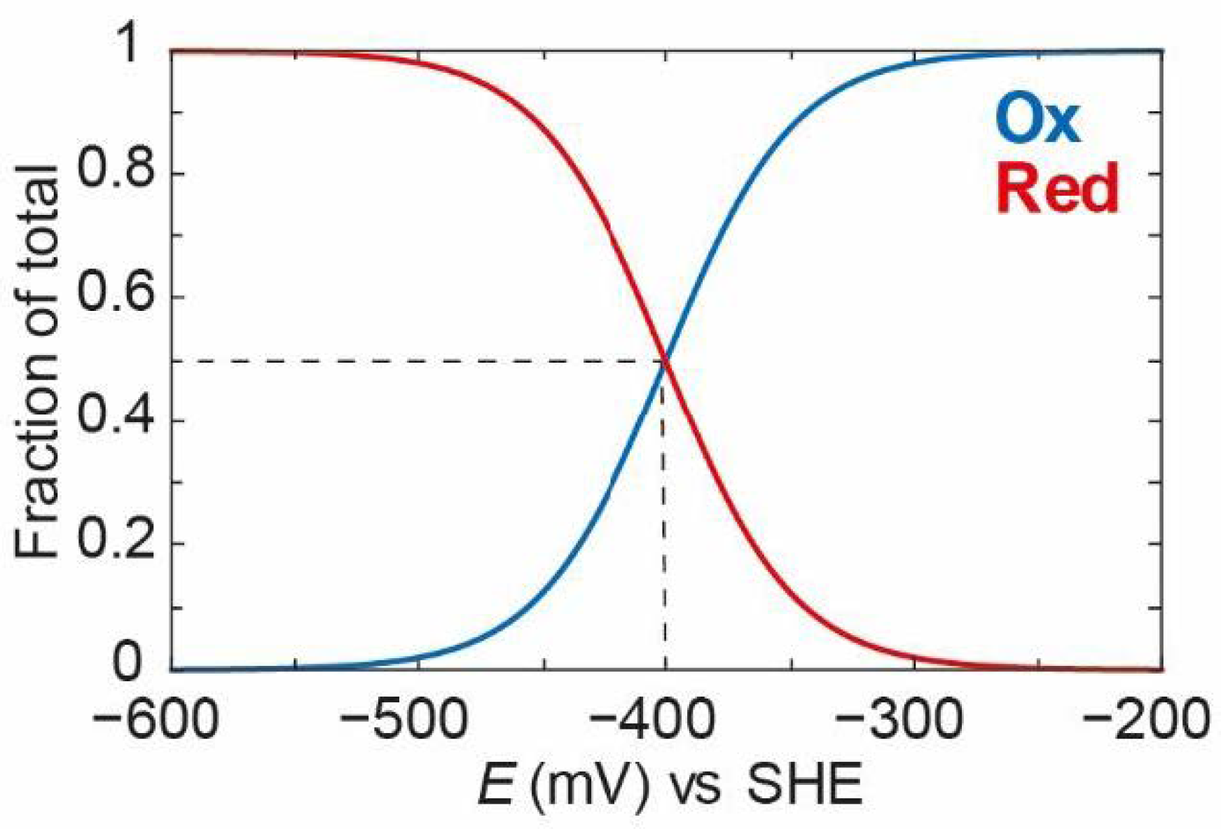
Plotting [Ox] (Equation (3)) and [Red] (Equation (2)) against the applied potential using an E^O value of −400 mV vs. SHE (chosen as an arbitrary potential close to the thermodynamic potential of the 2H⁺/H₂ couple at physiological pH) and n = 1 (indicating a single electron transferred), it then gives the curves shown in Figure 2. It can clearly be seen that, at a high applied potential (−200 mV) Ox dominates, and, as the applied potential decreases, Ox is converted gradually to Red with a middle point (the midpoint potential) of −400 mV.

Next, instead of assuming a redox event, we will assume a deprotonation event of a single cofactor with a single proton.

$$OxH\rightleftharpoons Ox+H^{+}$$

This situation is explained nicely by a simple acid dissociation constant (K_a):

$$K_a=\frac{\left[Ox\right]\left[H^{+}\right]}{\left[OxH\right]}$$

(4)

where K_a is the acid dissociation constant, [Ox] is the concentration of the deprotonated species, [H⁺] is the concentration of protons, and [OxH] is the concentration of the protonated species in M units.

$$\left[Ox\right]+\left[OxH\right]=1$$

$$\left[OxH\right]=1-\left[Ox\right]$$

(5)

Rearranging Equation (4), we get:

$$K_a\left[OxH\right]=\left[Ox\right]\left[H^{+}\right]$$

$$\left[OxH\right]=\left[Ox\right]\frac{\left[H^{+}\right]}{K_a}$$

Then [OxH] is substituted with Equation (5):

$$1-\left[Ox\right]=\left[Ox\right]\frac{\left[H^{+}\right]}{K_a}$$

$$1=\left[Ox\right]+\left[Ox\right]\frac{\left[H^{+}\right]}{K_a}$$

$$1=\left[Ox\right](1+\frac{\left[H^{+}\right]}{K_a})$$

$$\left[Ox\right]=\frac{1}{1+\frac{\left[H^{+}\right]}{K_a}}$$

Finally, this can be rearranged to express [Ox] in terms of the difference between the pK_a and the pH:

$${pK}_a=-{\log }_{10}(K_a)$$

$$\mathrm{pH}=-{\log }_{10}(\left[H^{+}\right])$$

$$K_a={10}^{-{pK}_a}$$

$$\left[H^{+}\right]={10}^{-\mathrm{pH}}$$

$$\left[Ox\right]=\frac{1}{1+\frac{{10}^{-\mathrm{pH}}}{{10}^{-{pK}_a}}}$$

$$\left[Ox\right]=\frac{1}{1+{10}^{(pKa-\mathrm{pH})}}$$

(6)

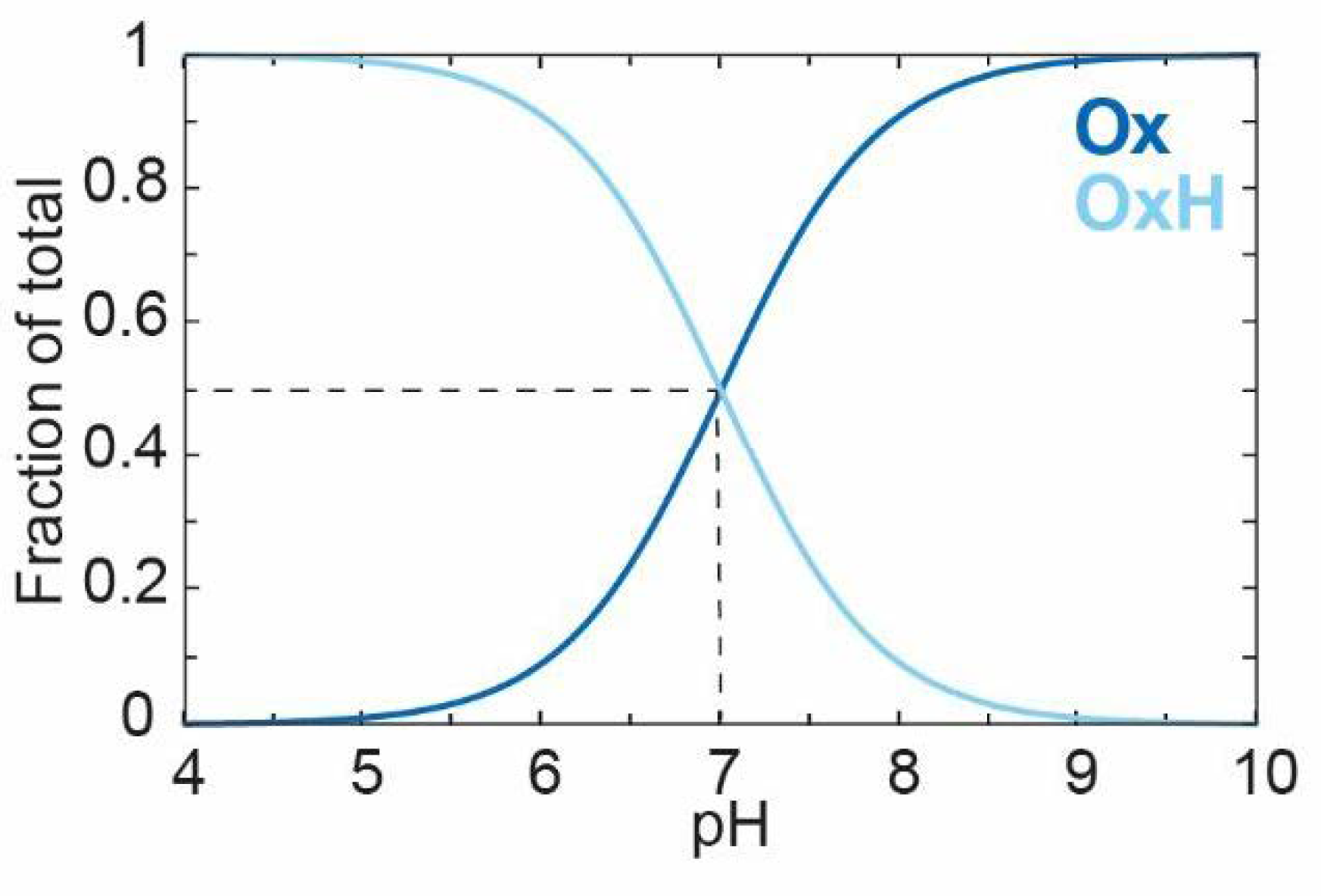
Plotting [Ox] (Equation (6)) and [OxH] (Equation (5)) against the pH using a K_a value of 10⁻⁷ (or a pK_a of 7) gives the curves shown in Figure 3. At a high pH, the deprotonated species Ox dominates, and, as the pH decreases, Ox converts gradually to OxH with a pK_a of 7.

2.2. Proton Coupled Electron Transfer

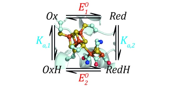
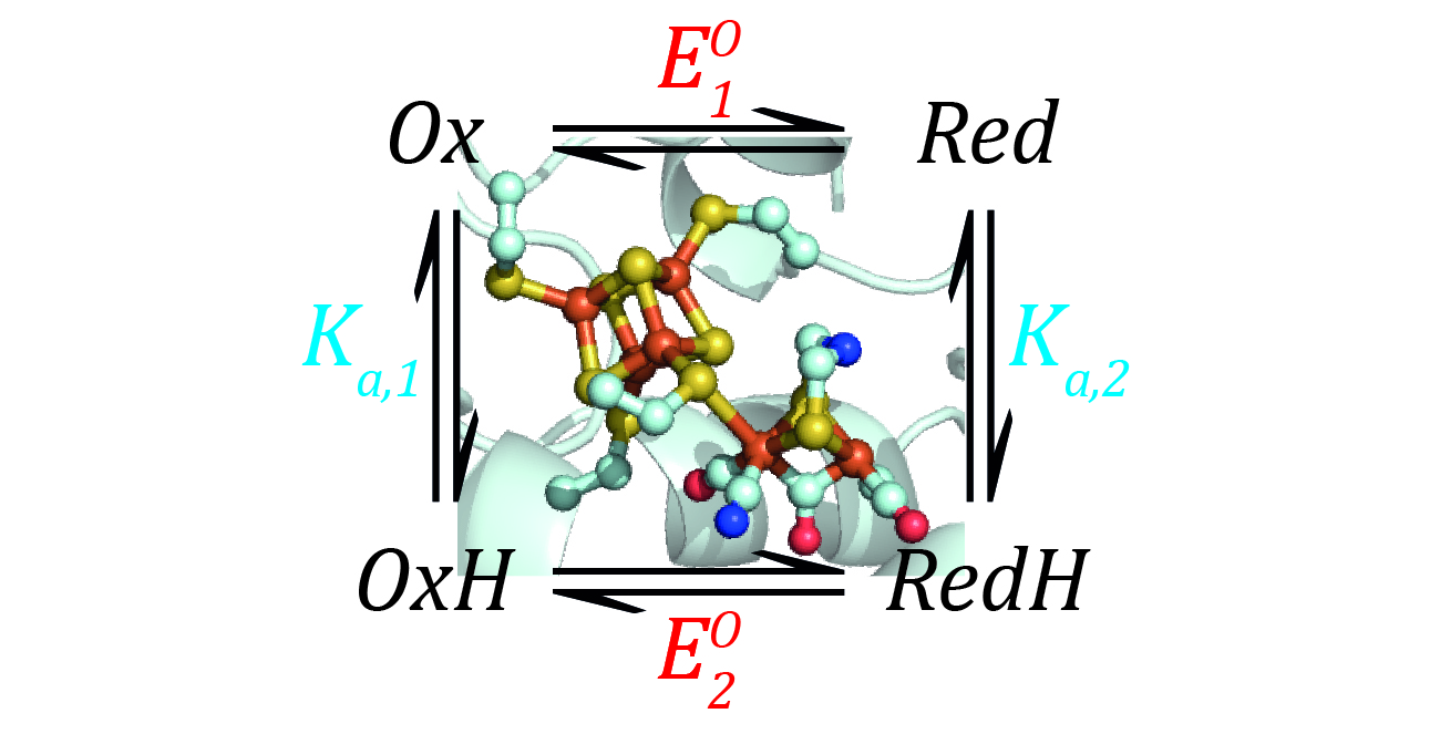
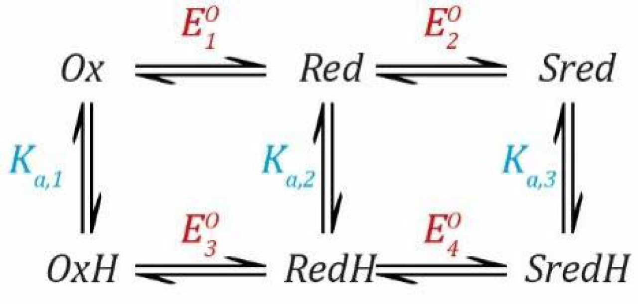
Now, we can combine both events into a thermodynamic model describing a species that can be protonated and reduced by one electron simultaneously, as shown in Scheme 1.

Now, we need to define two E^O values based on the Nernst Equation (1), including one for the deprotonated states (Ox and Red) and one for the protonated states (OxH and RedH), and two K_a values based on the simple acid dissociation constant Equation (4), one for the oxidised states (Ox and OxH) and one for the reduced states (Red and RedH). Here, as before, E refers to the applied potential to the system and, therefore, all redox couples are in equilibrium with this.

$$E=E_1^O-\frac{\mathrm{RT}}{\mathrm{nF}}\ln (\frac{\left[Red\right]}{\left[Ox\right]})$$

$$E=E_2^O-\frac{\mathrm{RT}}{\mathrm{nF}}\ln (\frac{\left[RedH\right]}{\left[OxH\right]})$$

$$K_{a,1}=\frac{\left[Ox\right]\left[H^{+}\right]}{\left[OxH\right]}$$

$$K_{a,2}=\frac{\left[Red\right]\left[H^{+}\right]}{\left[RedH\right]}$$

These equations can be rearranged to get everything in terms of [Ox] as follows.

$$\left[Red\right]=\left[Ox\right]\times \exp \frac{\mathrm{nF}}{\mathrm{RT}}(E_1^O-E)$$

$$\left[Red\right]=\left[Ox\right]\times \mathsf{\alpha }$$

(7)

where:

$$\mathsf{\alpha }=\exp \frac{\mathrm{nF}}{\mathrm{RT}}(E_1^O-E)$$

(8)

$$\left[RedH\right]=\left[OxH\right]\times \exp \frac{\mathrm{nF}}{\mathrm{RT}}(E_2^O-E)$$

$$\left[RedH\right]=\left[OxH\right]\times \mathsf{\beta }$$

(9)

where:

$$\mathsf{\beta }=\exp \frac{\mathrm{nF}}{\mathrm{RT}}(E_2^O-E)$$

(10)

$$\left[OxH\right]=\left[Ox\right]\frac{\left[H^{+}\right]}{K_{a,1}}$$

(11)

$$\left[RedH\right]=\left[Red\right]\frac{\left[H^{+}\right]}{K_{a,2}}$$

(12)

Again, we define the sum of the concentration of all states as 1.

$$\left[Ox\right]+\left[Red\right]+\left[OxH\right]+\left[RedH\right]=1$$

(13)

Next, we substitute [OxH] and [RedH] from Equations (11) and (12) into Equation (13).

$$\left[Ox\right]+\left[Red\right]+\left[Ox\right]\frac{\left[H^{+}\right]}{K_{a,1}}+\left[Red\right]\frac{\left[H^{+}\right]}{K_{a,2}}=1$$

$$\left[Ox\right]+\left[Ox\right]\frac{\left[H^{+}\right]}{K_{a,1}}+\left[Red\right]+\left[Red\right]\frac{\left[H^{+}\right]}{K_{a,2}}=1$$

$$\left[Ox\right](1+\frac{\left[H^{+}\right]}{K_{a,1}})+\left[Red\right](1+\frac{\left[H^{+}\right]}{K_{a,2}})=1$$

(14)

followed by substitution of [Red] from Equation (7) into Equation (14).

$$\left[Ox\right](1+\frac{\left[H^{+}\right]}{K_{a,1}})+\left[Ox\right]\times \mathsf{\alpha }(1+\frac{\left[H^{+}\right]}{K_{a,2}})=1$$

$$\left[Ox\right]\left\{1+\frac{\left[H^{+}\right]}{K_{a,1}}+\mathsf{\alpha }(1+\frac{\left[H^{+}\right]}{K_{a,2}})\right\}=1$$

$$\left[Ox\right]=\frac{1}{1+\frac{\left[H^{+}\right]}{K_{a,1}}+\mathsf{\alpha }(1+\frac{\left[H^{+}\right]}{K_{a,2}})}$$

As for Equation (6) from Section 2.1, this can be rearranged to express [H⁺], K_a,1, and K_a,2 as pH, pK_a,1, and pK_a,2.

$$\left[Ox\right]=\frac{1}{1+{10}^{({pK}_{a,1}-\mathrm{pH})}+\mathsf{\alpha }(1+{10}^{({pK}_{a,2}-\mathrm{pH})})}$$

(15)

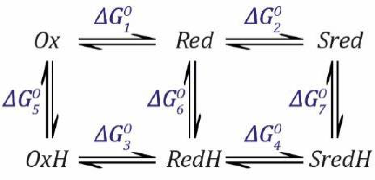
Importantly, in order to arrive at this result, we only need to consider the two protonation events defined by K_a,1 and K_a,2 and the reduction event defined by $E_1^O$. We can calculate $E_2^O$ by considering that the free energy change (ΔG) when going from Ox to RedH is the same, whether we go via Red or via OxH. We can define the situation (Scheme 2) as follows (remember that K_a,1 and K_a,2 are dissociation constants, so the free energy change ΔG is defined for this direction and must be subtracted when we go in the opposite direction).

The total free energy change when going from Ox to RedH is the same whether we go via Red or OxH ($\Delta G_3^O$ and $\Delta G_4^O$ are subtracted because they are defined for the deprotonation process).

$$\Delta G_1^O-\Delta G_4^O=\Delta G_2^O-\Delta G_3^O$$

(16)

Since:

$$\Delta G=-\mathrm{nF}E$$

$$\Delta G=-\mathrm{RTln}K$$

we can define the free energy changes for the reduction and deprotonation steps as follows.

$$\Delta G_1^O=-{\mathrm{nF}E}_1^O$$

(17)

$$\Delta G_2^O=-{\mathrm{nF}E}_2^O$$

(18)

$$\Delta G_3^O=-{\mathrm{RTln}K}_{a,1}$$

(19)

$$\Delta G_4^O=-{\mathrm{RTln}K}_{a,2}$$

(20)

which can then be substituted into Equation (16) and rearranged for $E_2^O$.

$$-{\mathrm{nF}E}_1^O-(-{\mathrm{RTln}K}_{a,2})=-{\mathrm{nF}E}_2^O-(-{\mathrm{RTln}K}_{a,1})$$

$$-{\mathrm{nF}E}_1^O+{\mathrm{RTln}K}_{a,2}=-{\mathrm{nF}E}_2^O+{\mathrm{RTln}K}_{a,1}$$

$${\mathrm{nF}E}_2^O={\mathrm{nF}E}_1^O+{\mathrm{RTln}K}_{a,1}-{\mathrm{RTln}K}_{a,2}$$

$$E_2^O=E_1^O+\frac{\mathrm{RT}}{\mathrm{nF}}\ln \frac{K_{a,1}}{K_{a,2}}$$

(21)

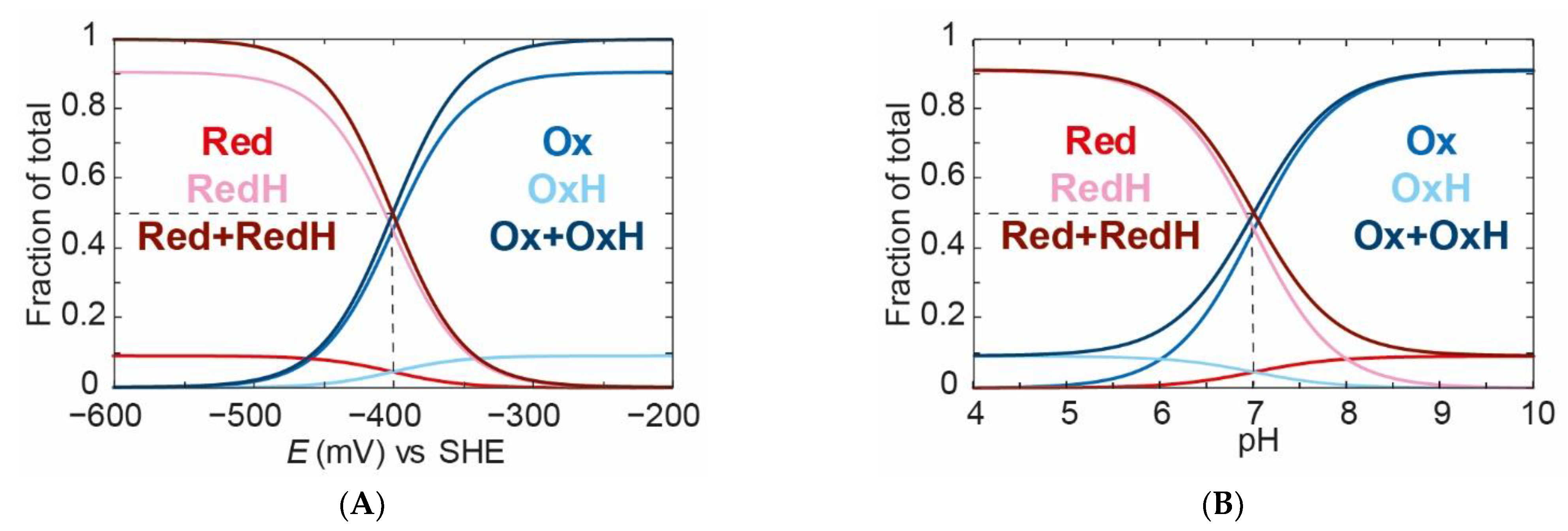
Using this simple model, we can plot the dependence of each of the species Ox, Red, OxH, and RedH as a function of either the applied potential at a given pH (Figure 4A) or as a function of the pH at a given applied potential (Figure 4B).

We can see that, at a fixed pH value of 7 (Figure 4A), when we titrate the applied potential from high (less negative) to low (more negative), we go from about 90% Ox and 10% OxH to about 10% Red and 90% RedH. A crucial observation needs to be made at this stage: all species titrate with an identical “apparent” midpoint potential of −400 mV. This is because the redox and protonation events are coupled. Importantly, the Ox:OxH ratio and the Red:RedH ratio do not change with the applied potential. This may seem clear, but a lack of understanding of this concept could lead to erroneous conclusions.

Similarly, if we titrate the pH from high to low at a constant applied potential of −400 mV (Figure 4B), we can see that we go from a mixture of 90% Ox and 10% Red to a mixture of 10% OxH and 90% RedH with an “apparent” pK_a of 7. This is an important observation in which we have shown that the redox state is dependent on the pH. This indicates the presence of a proton coupled electron transfer (PCET). 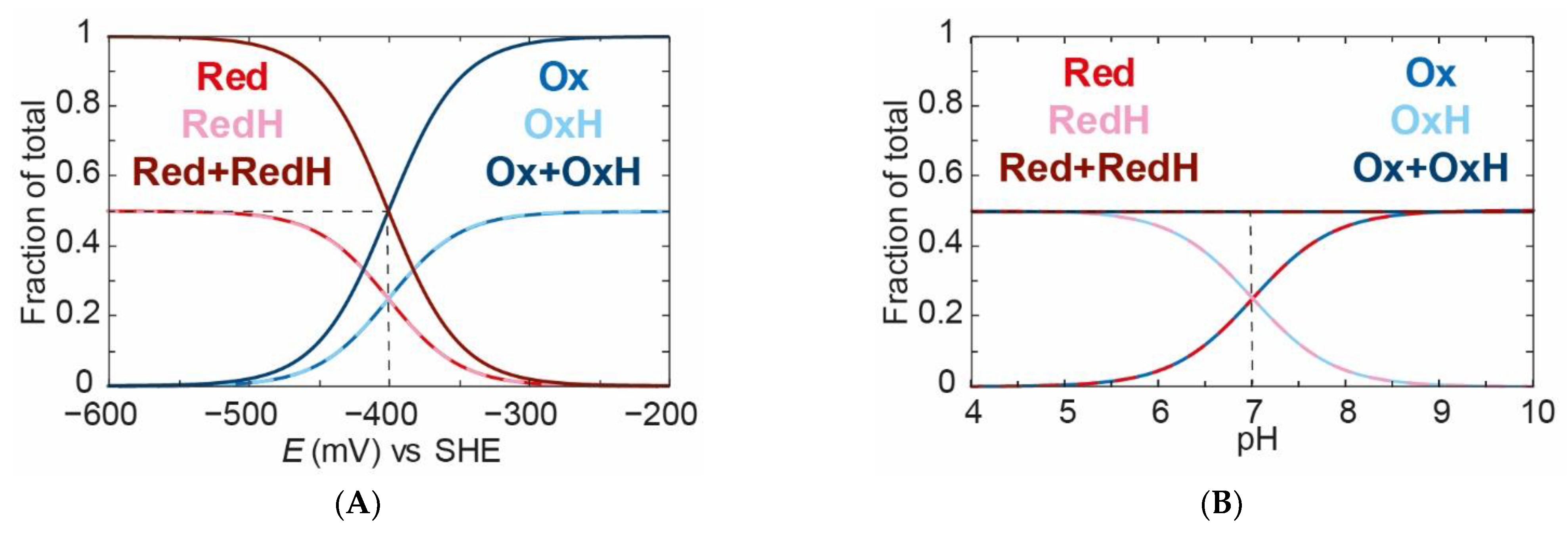The reason for this is that we have chosen different pK_a values for the oxidised and reduced species. If we had identical pK_a values for the oxidised and reduced species, then no PCET would occur. This situation is shown in Figure 5A,B, where the pK_a values are both 7. Since the applied potential is titrated from high to low, a 50% mixture of Ox and OxH converts to a 50% mixture of Red and RedH with an “apparent” midpoint potential of −400 mV vs. SHE. In Figure 5B, the total oxidised species (Ox + OxH) to the total reduced species (Red + RedH) ratio does not change with pH, indicating no PCET. However, it can be seen that Ox titrates to OxH and Red titrated to RedH as the pH is changed from high to low.

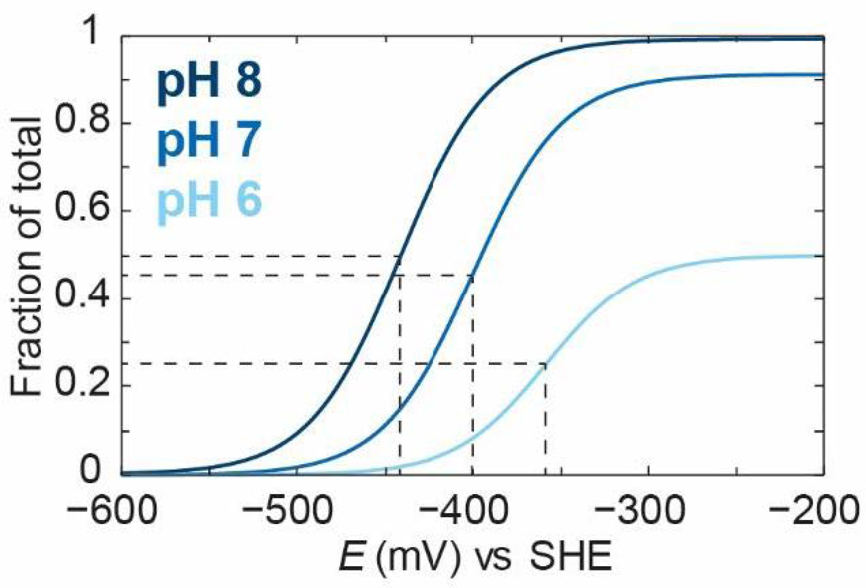
To emphasise the crucial observation that “apparent” redox potentials can shift with pH for the case where we have different pK_a values for Ox and Red, one can compare the titrations of the Ox species at three pH values (Figure 6).

As can be seen from Figure 6, the “apparent” midpoint potential for the titration of Ox shifts with pH, even if the change of Ox to Red itself does not directly involve a proton. However, the fundamental point is that the ratio between the Ox and OxH species will be the same at every value of the applied potential (as long as the pH is fixed). This is because the ratio between Ox and OxH is determined only by the acid dissociation constant K_a,1. 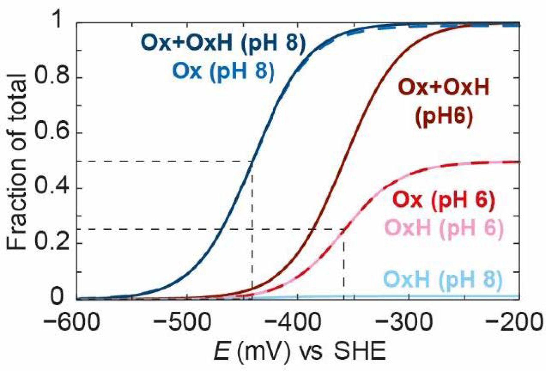Thus, if the process of proton-coupled reduction of Ox to RedH can occur, then the titration of the total amount of the oxidised species (Ox + OxH) and the titration of the total amount of the reduced species (Red + RedH), will change with pH. It must, therefore, be the case that the titration of the component states changes with pH. To illustrate this, Figure 7 shows the titration of Ox, OxH, and Ox + OxH at pH 6 and pH 8. It is clear that, at pH 6, the Ox state titrates with a more positive “apparent” redox potential than at pH 8. The components Ox and OxH species titrate with the same potential at pH 6. At pH 8, only the Ox state can be observed since its pK_a is too low to observe OxH at this pH.

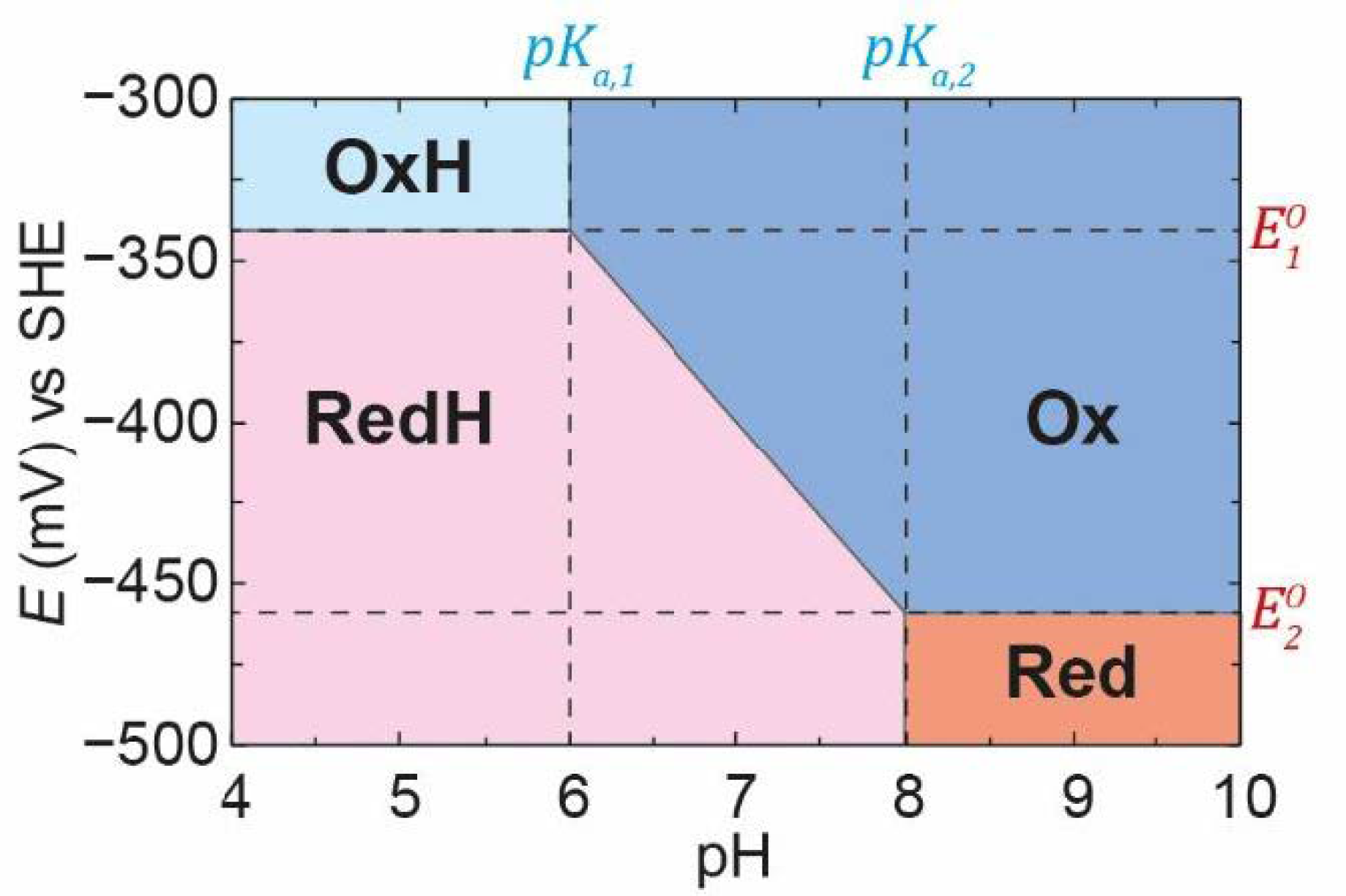
Using the $E_1^O$, $E_2^O$, pK_a,1, and pK_a,2 values defined in Figure 4, for a PCET process, we can plot the famous Pourbaix diagram [40] in which the regions of stability of each of the species Ox, OxH, Red, and RedH are defined (Figure 8). It should be recognised, however, that the boundaries between each of these regions do not represent step functions but represent the smooth titrations between each state. For example, it can be seen in Figure 4 that, at pH 7 and E = −400 mV (a point right in the middle of the Pourbaix diagram in Figure 8), we have about 45% Ox, 45% RedH, 5% OxH, and 5% Red. Thus, we still observe OxH and Red even though we are outside of the regions where these states are defined as stable in the Pourbaix diagram.

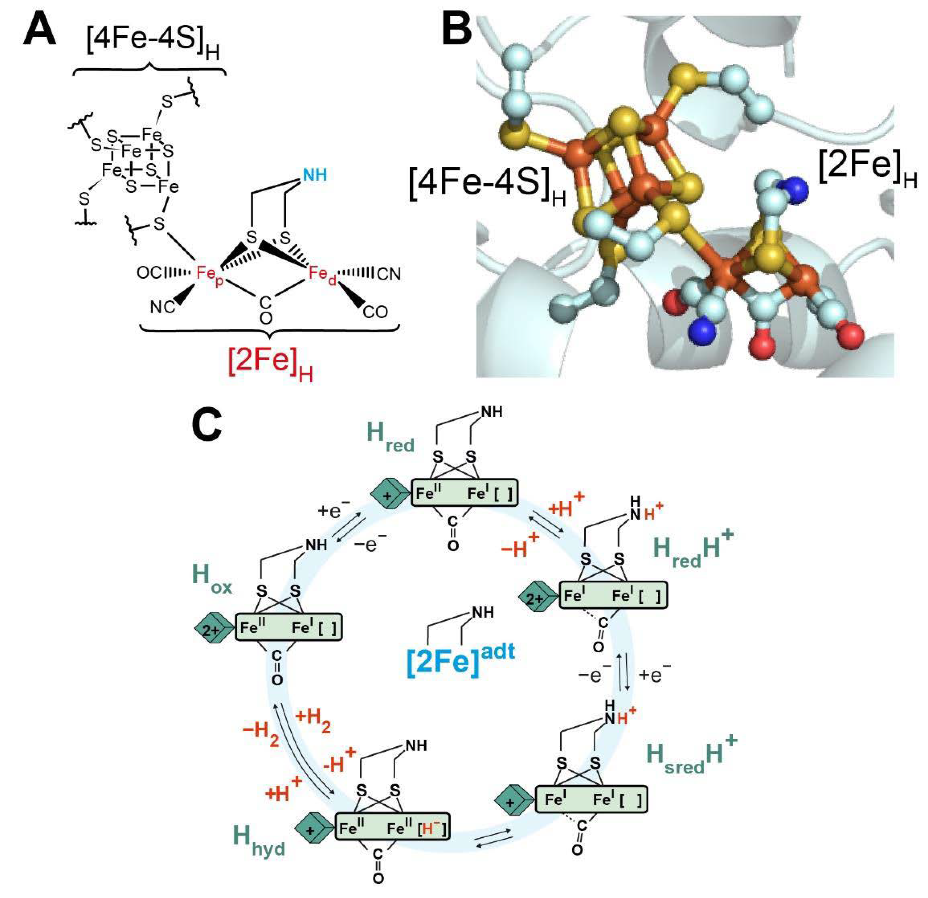
2.3. A Simple Model for the [FeFe] Hydrogenase

Experimental data show that the simplest [FeFe] hydrogenase, CrHydA1, containing only the H-cluster and no additional F-clusters, can be reduced by two electrons. The most oxidised state H_ox gets reduced by one electron to form H_red, and H_red can subsequently be reduced by a second electron to yield H_sred [41,42].

$$H_{ox}+2e^{-}\rightleftharpoons H_{red}+e^{-}\rightleftharpoons H_{sred}$$

It was shown that photoexcitation of frozen samples of the H_red state gave a different form of H_red, which was named H_red’ [43]. Around the same time, it was noted that H_red’ dominated at high pH, while H_red dominated at low pH [35]. Furthermore, it was observed that only the H_red’ state formed in the PDT variant of CrHydA1 (which lacks a protonatable dithiolate ligand in [2Fe]_H) [38]. The simplest interpretation of the data was that the electron could reside mostly on the [4Fe-4S]_H subcluster, or mostly on the [2Fe]_H subcluster, and that protonation of the ADT bridging nitrogen from NH to NH₂⁺ was the event that triggered the electronic rearrangement. Thus, the H_red’ and H_red states were renamed H_red and H_redH⁺, respectively [35]. Moreover, based on the fact that H_sred cannot be formed in the PDT variant of CrHydA1 [38], it was assumed that H_sred should be in a protonated state, and was named H_sredH⁺. To describe this situation, a more complex model is required including two redox steps and one protonation step.

In Section 2.2, we described a simple model for proton coupled electron transfer in which four states exist: Ox, OxH, Red, and RedH. Now, we will extend this model to include a second redox event (Scheme 3).

This creates a total of six states connected by seven steps. In this model, Ox is the most oxidised state, Red is the one electron reduced state, and Sred is the two-electron reduced state or “super-reduced” state. Each of these unprotonated states has a protonated counterpart: OxH, RedH, and SredH. Importantly, nothing about this model indicates the location of redox or (de)protonation events because we have a system that can accept two electrons and one proton. One could also consider a model involving one redox and two (de)protonation events, or even two redox and two (de)protonation events. However, the former does not fit at all with experimentally observed spectro-electrochemical titrations, as two redox steps are clearly discerned, while the latter leads to a reactive state that can release H₂ [35,42]. To make a 2e⁻/2H⁺ model reversible, an H₂ binding/dissociation step is required, which would complicate the model. Nevertheless, the simple 2e⁻/1H⁺ model has been shown to accurately describe pH-dependent spectro-electrochemical titrations [35]. The equations describing this model can be derived using the Nernst Equation (1) and the equation for a simple acid dissociation constant (4) by analogy to those in Section 2.2.

$$E=E_1^O-\frac{\mathrm{RT}}{\mathrm{nF}}\ln (\frac{\left[Red\right]}{\left[Ox\right]})$$

$$E=E_2^O-\frac{\mathrm{RT}}{\mathrm{nF}}\ln (\frac{\left[Sred\right]}{\left[Red\right]})$$

$$E=E_3^O-\frac{\mathrm{RT}}{\mathrm{nF}}\ln (\frac{\left[RedH\right]}{\left[OxH\right]})$$

$$E=E_4^O-\frac{\mathrm{RT}}{\mathrm{nF}}\ln (\frac{\left[SredH\right]}{\left[RedH\right]})$$

$$K_{a,1}=\frac{\left[Ox\right]\left[H^{+}\right]}{\left[OxH\right]}$$

$$K_{a,2}=\frac{\left[Red\right]\left[H^{+}\right]}{\left[RedH\right]}$$

$$K_{a,3}=\frac{\left[Sred\right]\left[H^{+}\right]}{\left[SredH\right]}$$

As previously done, these equations can be rearranged in terms of [Ox] (for a complete derivation, see the Supplementary Materials Section S1).

$$\left[Ox\right]=\frac{1}{1+\mathsf{\alpha }(1+\mathsf{\beta })+{10}^{({pK}_{a,1}-\mathrm{pH})}\left\{1+\mathsf{\gamma }(1+\mathsf{\delta })\right\}}$$

(22)

where:

$$\mathsf{\alpha }=\exp \frac{\mathrm{nF}}{\mathrm{RT}}(E_1^O-E)$$

(23)

$$\mathsf{\beta }=\exp \frac{\mathrm{nF}}{\mathrm{RT}}(E_2^O-E)$$

(24)

$$\mathsf{\gamma }=\exp \frac{\mathrm{nF}}{\mathrm{RT}}(E_3^O-E)$$

(25)

$$\mathsf{\delta }=\exp \frac{\mathrm{nF}}{\mathrm{RT}}(E_4^O-E)$$

(26)

Although we did not need to use all the parameters to arrive at the results (K_a,2 and K_a,3 were not used), we can use the conjoined thermodynamic cycles in this model to derive further equations for these parameters. We can define the situation (Scheme 4) as follows.

The rules still apply so that the free energy change is the same regardless which pathway is taken. Thus, going from Ox to RedH via Red or via OxH have the same overall free energy change, as does going from Red to SredH via Sred or via RedH. Therefore, we can define the following equations.

$$\Delta G_1^O-\Delta G_6^O=\Delta G_3^O-\Delta G_5^O$$

$$\Delta G_2^O-\Delta G_7^O=\Delta G_4^O-\Delta G_6^O$$

where:

$$\Delta G_1^O=-{\mathrm{nF}E}_1^O$$

$$\Delta G_2^O=-{\mathrm{nF}E}_2^O$$

$$\Delta G_3^O=-{\mathrm{nF}E}_3^O$$

$$\Delta G_4^O=-{\mathrm{nF}E}_4^O$$

$$\Delta G_5^O=-{\mathrm{RTln}K}_{a,1}$$

$$\Delta G_6^O=-{\mathrm{RTln}K}_{a,2}$$

$$\Delta G_7^O=-{\mathrm{RTln}K}_{a,3}$$

These equations can then be combined to find expressions for K_a,2 and K_a,3 (see SI Section S1 for complete derivations). The final results are shown here:

$$K_{a,2}=K_{a,1}\exp \{\frac{\mathrm{nF}}{\mathrm{RT}}(E_1^O-E_3^O)\}$$

(27)

$$K_{a,3}=K_{a,2}\exp \{\frac{\mathrm{nF}}{\mathrm{RT}}(E_2^O-E_4^O)\}$$

(28)

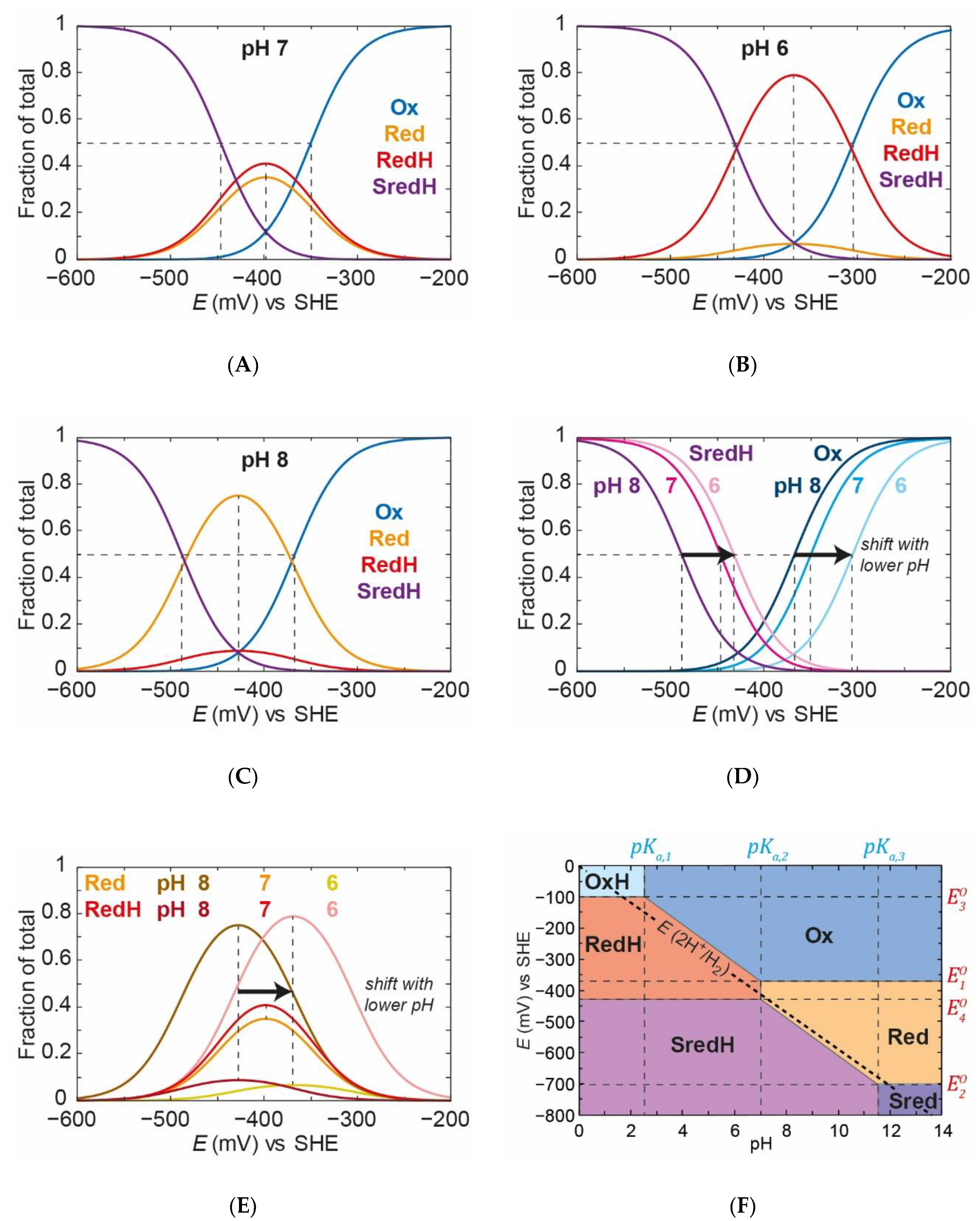
Using this model, the populations of all the states can be varied as a function of applied potential at various pH values (Figure 9). As can be seen from Figure 9A, for pH 7, at a high applied potential, only the Ox state exists. The Ox/OxH transition has such a low pK_a value (2.5) that, at pH 7, the OxH state is essentially completely deprotonated and only Ox exists. As the applied potential is decreased, the Ox state decreases in population (with an apparent midpoint potential of −350 mV) and the Red and RedH states come up with roughly equal proportions, reaching a maximum concentration at around −400 mV vs. SHE. In this case, the pK_a for the Red/RedH transition is ≈7.1, which is why the amount of RedH is slightly higher than that of Red. As the applied potential decreases even further, Red and RedH are both converted to SredH (with an apparent midpoint potential of −450 mV). The pK_a for the Sred/SredH transition is ≈11.6, which means that the Sred state is essentially completely protonated to SredH at pH 7.

At pH 6 (Figure 9B) and 8 (Figure 9C), similar behaviour can be observed. At pH 6, the Ox state is converted to Red and RedH with a higher apparent midpoint potential (−300 mV) than at pH 7 (−350 mV). The Red state is mostly protonated to RedH, and the Red and RedH states are reduced to SredH with a higher apparent midpoint potential (−430 mV) than at pH 7 (−450 mV). At pH 8, the Ox state is converted to Red and RedH with a lower apparent midpoint potential (−370 mV) than at pH 7 (−350 mV). The RedH state is mostly deprotonated to Red, and the Red and RedH states are reduced to SredH with a lower apparent midpoint potential (−480 mV) than at pH 7 (−450 mV).

In Figure 9D, the behaviours of Ox and SredH are compared at the three pH values. There is a clear observation that the titrations of both species are affected by pH. This is intuitive because the reduction of Ox can occur with or without protonation to give RedH and Red, respectively, with the former requiring a proton. Likewise, reduction of Red to SredH requires protonation, while reduction of RedH to SredH does not. In Figure 9E, the behaviours of Red and RedH are compared at the three pH values. Again, both species appear to be affected by pH. The appearance of RedH and the disappearance of Red should be pH dependent. What is possibly less intuitive is that the appearance of Red and the disappearance of RedH also appear to be pH dependent. This is caused by the fact that Red and RedH are in an equilibrium set by the pK_a,2 value and the pH. Thus, whatever happens to Red must also apply to RedH and vice versa. This means that a simple analysis of how the maximum populations of Red and RedH shift with pH (see Supplementary Discussion in Reference [36]) could erroneously lead to the conclusion that there are two separate proton coupled electron transfer events, including one to make Red and one to make RedH. This can be seen even more clearly in Figure 9F, where we have plotted a Pourbaix diagram for this model. Between the limits of the pK_a,1 (2.5) and pK_a,2 (7.1), the midpoint potential of Ox and OxH converting to Red and RedH is pH dependent. Likewise, between the limits of pK_a,2 and pK_a,3, the midpoint potential of Red and RedH converting to Sred and SredH is also dependent on pH.

In Figure 9, the pK_a values and intrinsic redox potentials have been set to ensure a situation where the OxH state is always deprotonated to Ox, while the Sred state is always protonated to SredH and the intermediate Red(H) state is a mixture of the protonated (RedH) and deprotonated (Red) forms (around physiological pH). This situation appears to most accurately reflect the behaviour of the [FeFe] hydrogenase from CrHydA1 [35]. 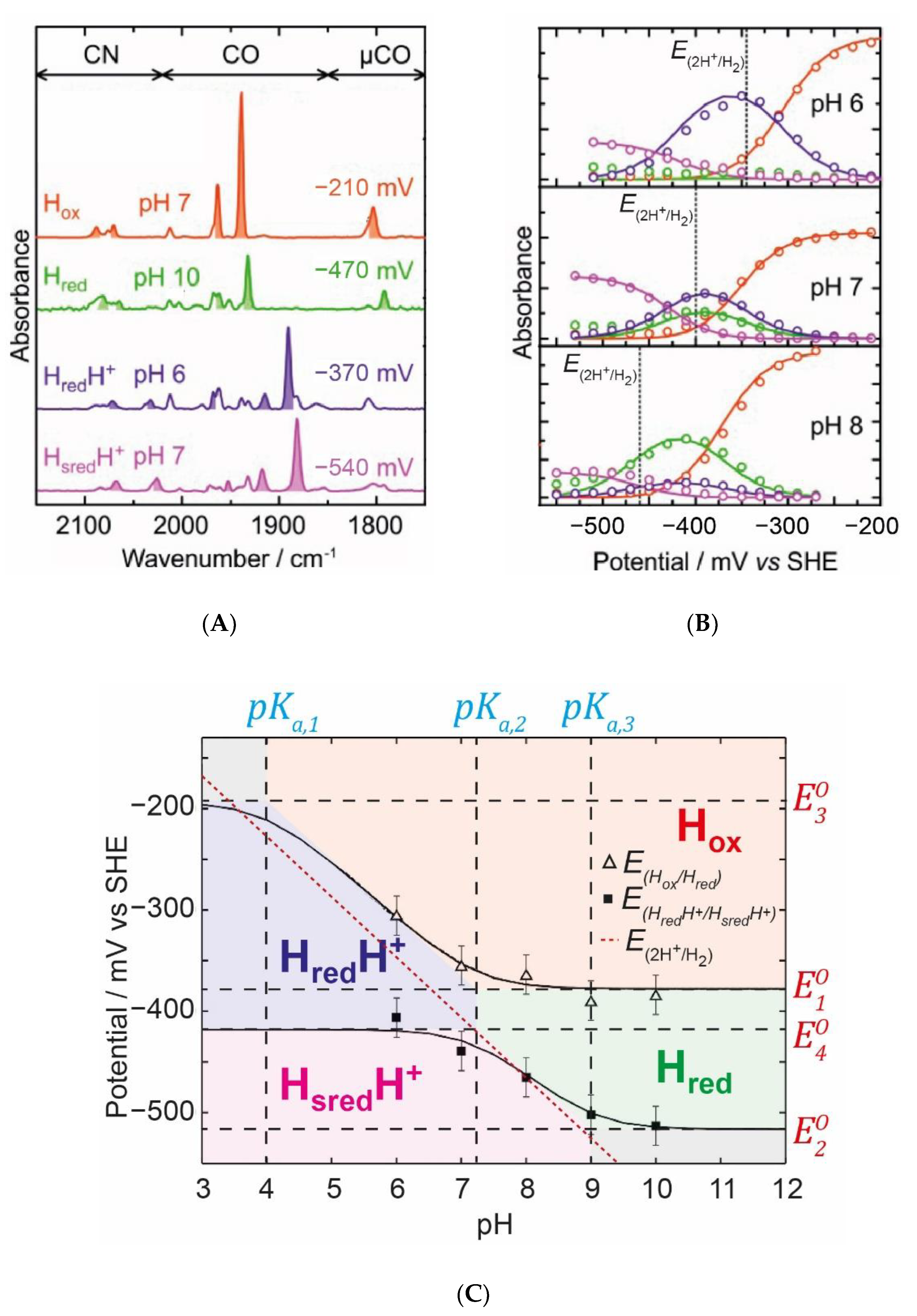In Figure 10, we exemplify how this thermodynamic model was employed by Sommer et al. to fit the IR spectro-electrochemical data obtained for the CrHydA1 hydrogenase at various pH values [35]. Figure 10A shows typical IR spectra under specific conditions that highlight the main catalytic states: H_ox, H_red, H_redH⁺, and H_sredH⁺. Figure 10B shows electrochemical titrations of the most dominant IR band in each of these states at pH 6, 7, and 8. It can clearly be seen that, as the pH increases, the titration curves shift to a more negative potential. The H_redH⁺ state becomes less abundant and the H_red state becomes more abundant. This behaviour seems very logical and fits the requirements of a reversible enzyme. Around neutral pH and the thermodynamic 2H⁺/H₂ potential, the enzyme is in a roughly equal mixture of both Red (H_red) and RedH (H_redH⁺) states, maximising the concentrations of both and, thereby, maximising the rates of oxidation of Red to Ox and reduction of RedH to SredH. If, instead, we imagine a situation where all redox states are deprotonated and only Ox, Red, and Sred exist, then one expects H₂ oxidation to be efficient, but H⁺ reduction will be inefficient. Likewise, if all states are protonated, H⁺ reduction is efficient but H₂ oxidation is not.

Effectively, the enzyme is optimised so that the potentials of the Ox(H)/Red(H) and Red(H)/Sred(H) are as close as possible to the thermodynamic 2H⁺/H₂ potential. This can be seen again in the Pourbaix diagram (Figure 9F for the model and Figure 10C for the model applied to CrHydA1). The thermodynamic 2H⁺/H₂ potential is shown as a dotted line. It is clear that, at a neutral pH, both transitions (Ox(H)/Red(H) and Red(H)/Sred(H)) are close to the thermodynamic 2H⁺/H₂ potential. In Figure 10C, the midpoint potential of the H_ox/H_red and H_red/H_sred transitions are plotted against the pH and are fitted with curves based on the model described above, with areas coloured to indicate where the various states dominate (in analogy to Figure 9F). Ideally, both curves would fit perfectly to the 2H⁺/H₂ potential at all pH values. However, using this model, it is not possible to generate such curves. One expects, therefore, at extreme pH values, to start to observe deviations of the catalytic efficiency in one direction. At a low pH, we expect a slight overpotential from H⁺ reduction, while, at a high pH, we expect a slight overpotential for H₂ oxidation. This seems to fit well with the known behaviour of the [FeFe] hydrogenase from CrHydA1 in IR spectro-electro-chemical titrations [33,35,44,45], but, interestingly, not with those from more complex enzymes including accessory iron-sulfur clusters [32,34]. In order to understand the behaviour in these more complex enzymes, we first need to deal with the concept of redox anti-cooperativity.

2.4. Redox Anticooperativity Model

In Section 2.2, we dealt with what happens when we can oxidise/reduce and protonate/deprotonate simultaneously, but we could also have two simultaneous oxidation/reduction events. Such a situation could be used to describe two iron-sulfur clusters located close to one another. These two redox events may be independent (i.e., their redox potentials do not influence one another) or they may be dependent (i.e., their redox potentials influence one another) [46]. This influence can be positive or negative. If reduction of one cluster makes it easier to reduce the second cluster, this would give us redox cooperativity. If reduction of one cluster makes it more difficult to reduce the second cluster, this would give us redox anti-cooperativity. 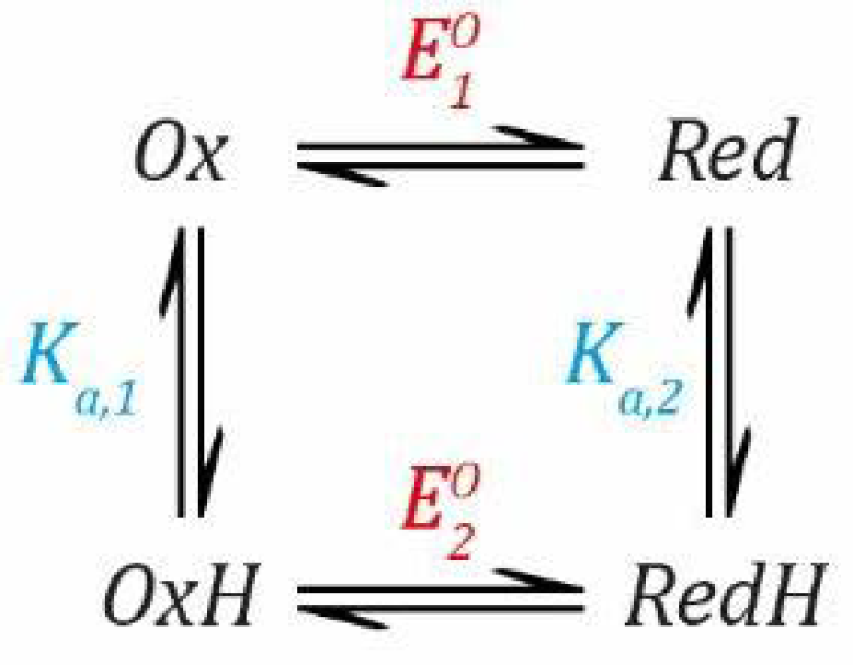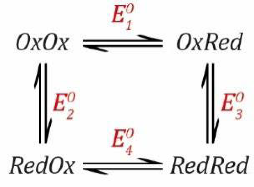Scheme 5 shows a simple model.

This situation is somewhat similar to the PCET scenario described in Section 2.2 except that it involves two electrons rather than one electron and one proton. All steps are redox steps and defined by the Nernst equation.

$$E=E_1^O-\frac{\mathrm{RT}}{\mathrm{nF}}\ln (\frac{\left[OxRed\right]}{\left[OxOx\right]})$$

$$E=E_2^O-\frac{\mathrm{RT}}{\mathrm{nF}}\ln (\frac{\left[RedOx\right]}{\left[OxOx\right]})$$

$$E=E_3^O-\frac{\mathrm{RT}}{\mathrm{nF}}\ln (\frac{\left[RedRed\right]}{\left[OxRed\right]})$$

$$E=E_4^O-\frac{\mathrm{RT}}{\mathrm{nF}}\ln (\frac{\left[RedRed\right]}{\left[RedOx\right]})$$

These equations can be rearranged to get everything in terms of [OxOx] (see SI Section S2 for a complete derivation).

$$\left[OxOx\right]=\frac{1}{1+\mathsf{\alpha }(1+\mathsf{\gamma })+\mathsf{\beta }}$$

(29)

where:

$$\mathsf{\alpha }=\exp \frac{\mathrm{nF}}{\mathrm{RT}}(E_1^O-E)$$

(30)

$$\mathsf{\beta }=\exp \frac{\mathrm{nF}}{\mathrm{RT}}(E_2^O-E)$$

(31)

$$\mathsf{\gamma }=\exp \frac{\mathrm{nF}}{\mathrm{RT}}(E_3^O-E)$$

(32)

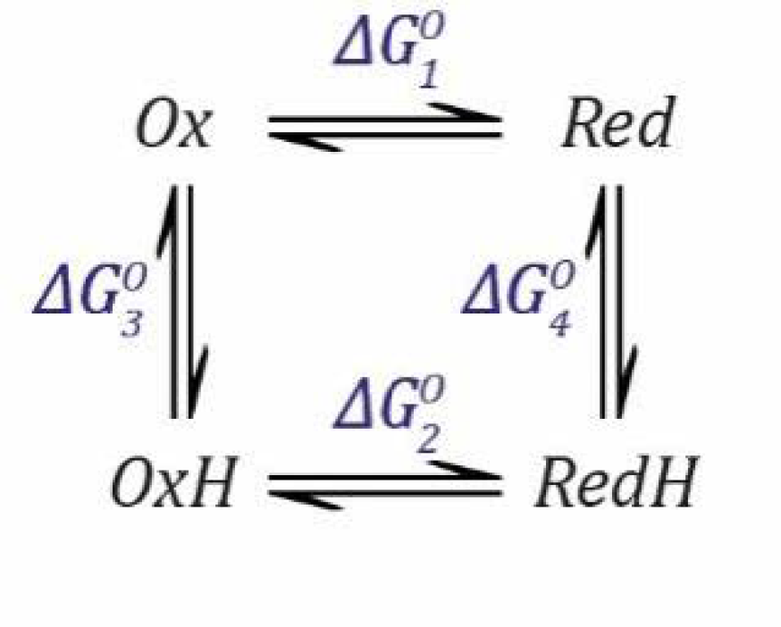
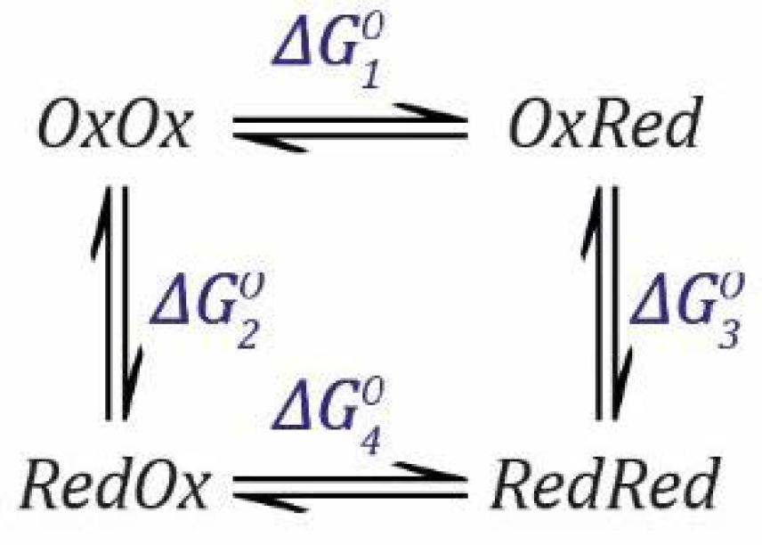
As before, in order to arrive at this result, we only need to consider the three reduction events defined by $E_1^O$, $E_2^O,$ and $E_3^O$. $E_4^O$ can be calculated considering the thermodynamic square (Scheme 6) as follows.

The rules still apply so that the free energy change is the same regardless which pathway is taken. Thus, going from OxOx to RedRed via OxRed or via RedOx have the same overall free energy change. Therefore, we can define the following equation.

$$\Delta G_1^O+\Delta G_3^O=\Delta G_2^O+\Delta G_4^O$$

(33)

where:

$$\Delta G_1^O=-{\mathrm{nF}E}_1^O$$

$$\Delta G_2^O=-{\mathrm{nF}E}_2^O$$

$$\Delta G_3^O=-{\mathrm{nF}E}_3^O$$

$$\Delta G_4^O=-{\mathrm{nF}E}_4^O$$

These equations can then be substituted into Equation (33) and rearranged to give $E_4^O$.

$$-{\mathrm{nF}E}_1^O+(-{\mathrm{nF}E}_3^O)=-{\mathrm{nF}E}_2^O+(-{\mathrm{nF}E}_4^O)$$

$${\mathrm{nF}E}_1^O+{\mathrm{nF}E}_3^O={\mathrm{nF}E}_2^O+{\mathrm{nF}E}_4^O$$

$${\mathrm{nF}E}_4^O={\mathrm{nF}E}_1^O-{\mathrm{nF}E}_2^O+{\mathrm{nF}E}_3^O$$

$$E_4^O=E_1^O-E_2^O+E_3^O$$

(34)

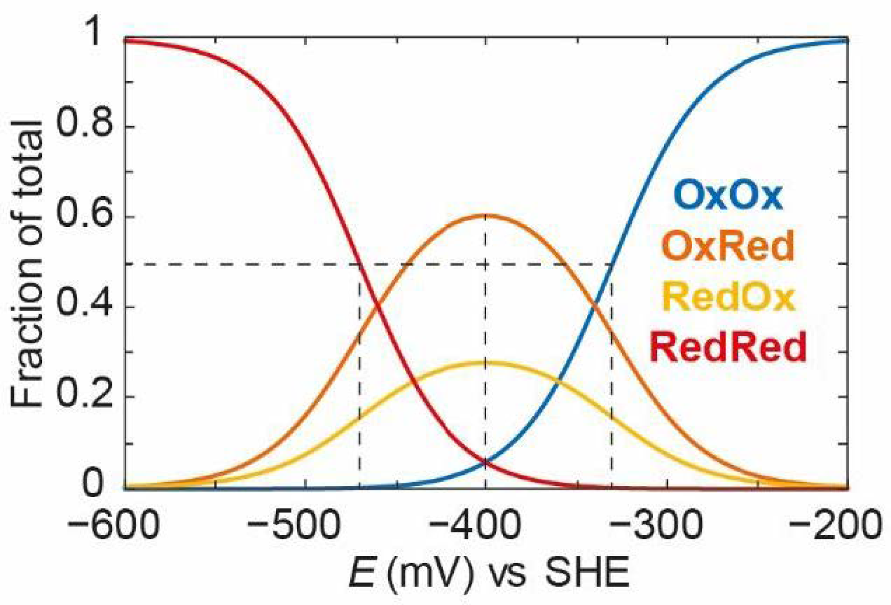
Now, we can set up two different situations, one in which we have two independent redox events (i.e., $E_1^O$= $E_4^O$ and $E_2^O$ = $E_3^O$) and one in which the redox events are dependent (i.e., $E_1^O$ ≠ $E_4^O$ and $E_2^O$ ≠ $E_3^O$). In Figure 11, the independent situation is shown where $E_1^O$ = $E_4^O$ = −390 mV and $E_2^O$ = $E_3^O$ = −410 mV (the average E^O is −400 mV).

It can be seen that, as the potential goes from positive to negative, OxOx decreases and both OxRed and RedOx increase. One can think of this as a single electron entering the enzyme and equilibrating between both clusters depending on their intrinsic redox potentials. In this case, OxRed is more dominant because it has a more positive redox potential (−390 mV vs. −410 mV). It should also be noted that the decrease in the OxOx state follows a titration with an “apparent” midpoint potential more positive than −390 mV. In fact, the “apparent” midpoint potential is −380 mV. This is because both the OxOx/OxRed and OxOx/RedOx couples are titrating at the same time. This means that the OxOx species is lost at slightly more positive potentials than the values of $E_1^O$ and $E_2^O$. The take-home message here is that these systems often behave in ways that, at first glance, seem non-intuitive, and it is only by studying the models that it is possible to fully understand their behaviour. As the second electron enters the enzyme, it will equilibrate among the remaining oxidised clusters and both OxRed and RedOx start to decrease as RedRed increases. RedRed increases with an “apparent” midpoint potential of −420 mV, which is slightly more negative than the values of $E_3^O$ and $E_4^O$.

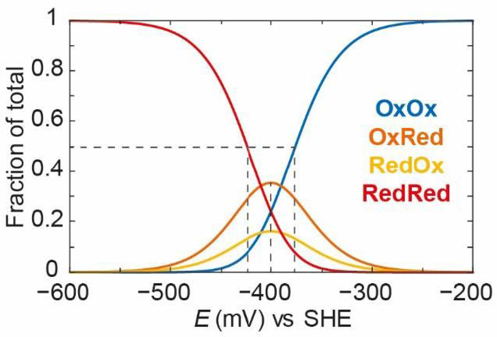
Next, we can apply the same model but introduce some redox anti-cooperativity. In Figure 12, we have defined $E_4^O$ = $E_1^O$ − 100 mV, i.e., there is 100 mV of redox anti-cooperativity, or the redox potential of one cluster is 100 mV more negative when the other cluster is reduced. Because of the thermodynamic square, this also means that $E_3^O$ = $E_2^O$ − 100 mV, and the redox potential of the second cluster is also 100 mV more negative when the other cluster is reduced. We have redefined the intrinsic redox potentials $E_1^O$ = −340 mV and $E_2^O$ = −360 mV so that the average E^O is still −400 mV, as in Figure 11.

As can be observed, OxOx decreases with a very positive “apparent” midpoint potential (−330 mV). OxRed and RedOx increase to a much greater extent and persist for longer until the RedRed state starts to increase with an “apparent” midpoint potential of −470 mV. These “apparent” midpoint potentials are 50 mV more positive and more negative, respectively, than those observed in Figure 11, reflecting the 100 mV redox anti-cooperativity.

This model was used to fit IR spectro-electrochemistry data from the [FeFe] hydrogenase from Desulfovibrio desulfuricans (DdHydAB) [34]. For the sake of brevity, we have not reproduced the fitting of the experimental data in this review. However, the interested reader is highly recommended to read Reference [34], where the simple anti-cooperativity model was applied to DdHydAB with PDT in the [2Fe] cluster. This enzyme possesses the active site H-cluster as well as two accessory iron-sulfur clusters (F-clusters). Unusual behaviour was observed in IR spectro-electrochemical redox titrations of this enzyme in which the active site had been artificially matured with a diiron cluster containing PDT. Since PDT cannot be protonated at the bridgehead atom, reduction only occurs at the [4Fe-4S]_H subcluster of the H-cluster giving small (5–10 cm⁻¹) shifts in the CO and CN⁻ bands to lower energy. These titrations showed non-Nernstian behaviour that indicated reduction of the proximal F-cluster caused the redox potential of the [4Fe-4S]_H to become more negative. In fact, the reduction of the proximal F-cluster could be observed directly as minute (<2 cm⁻¹) shifts in the IR bands of both the H_ox and H_red states. These data were fitted using the redox anti-cooperativity model described above and yielded a value of 118 mV for the interaction between the two clusters. This demonstrates that the modelling approach described in this case is not only illustrative but also practically useful for understanding spectro-electrochemical data and studying enzyme mechanisms. Since the PDT cofactor cannot be protonated, this simplified the number of redox states observed, and allowed the redox anti-cooperativity model to be investigated. However, to fully understand the behaviour of the natural H-cluster containing ADT in an F-cluster containing [FeFe] hydrogenase, it is necessary to incorporate redox anti-cooperativity into the full H-cluster model described in Section 2.3. In the next section, this is exactly what we will do.

2.5. Redox Anticooperativity Model for the Active [FeFe] Hydrogenase

In Section 2.1, we laid the foundations, showing the behaviour of a simple one electron redox and (de)protonation events. In Section 2.2, we combined redox and (de)protonation into a proton-coupled electron transfer model. Then, in Section 2.3, we added a second redox step to build a simple model that can be used to describe thermodynamic titrations of the H-cluster in the F-cluster free [FeFe] hydrogenase CrHydA1. 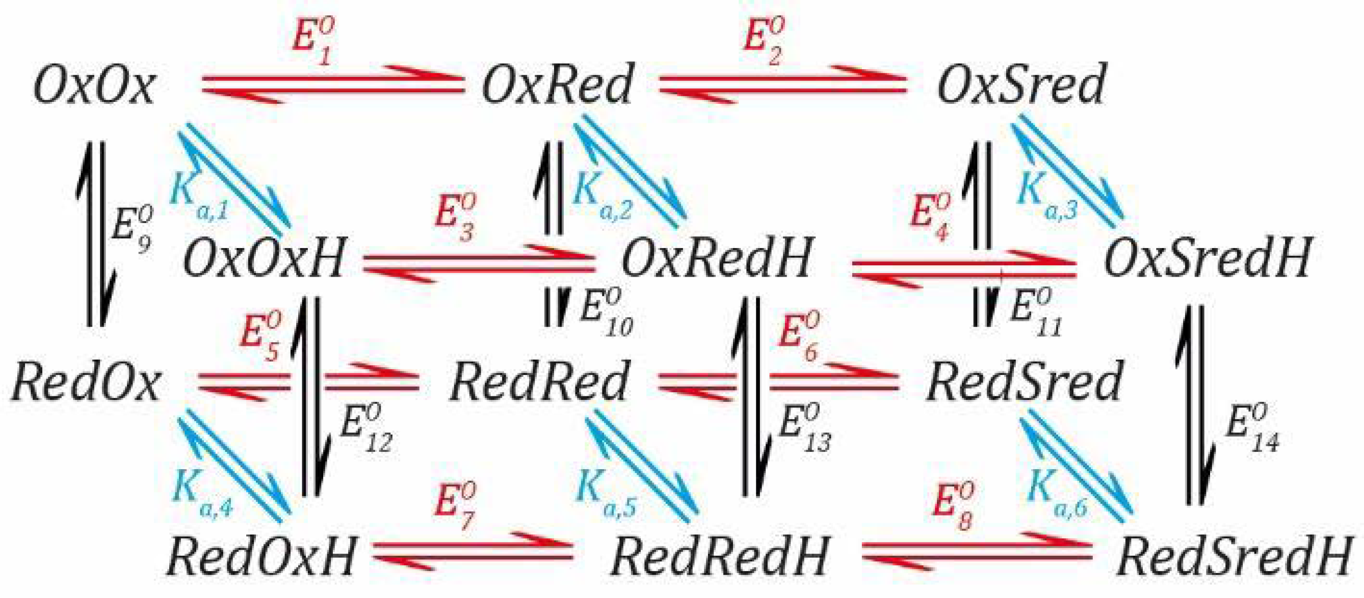In Section 2.4, we took a detour to look at what happens when two redox events occur adjacent to one another and can influence each other by redox anti-cooperativity. Now, we will combine what we have learned to build up a highly complex model containing both PCET and redox anti-cooperativity. Each species can now exist in three redox states of the H-cluster (Ox, Red, and Sred), two protonation states, and also two different redox states of the proximal F-cluster, making the model “three-dimensional” (Scheme 7).

As before, each E^O value defines the Nernst relationship between a reduced and an oxidised species and each K_a value defines the relationship between a protonated and a deprotonated species. Once all the equations are described for each pathway, they can all be rearranged to get everything in terms of [OxOx] (for the full derivation, please refer to the Supplementary Materials Section S3). Here, we will simply present the final equation for [OxOx] in terms of E^O values and K_a values, in all its complexity.

$$\left[\mathit{OxOx}\right]=\frac{1}{1+{\mathsf{\alpha }}_1(1+{\mathsf{\alpha }}_2)+{10}^{({pK}_{a,1}-\mathrm{pH})}\left\{1+{\mathsf{\alpha }}_3(1+{\mathsf{\alpha }}_4)\right\}+{\mathsf{\alpha }}_9(1+{\mathsf{\alpha }}_5(1+{\mathsf{\alpha }}_6)+{10}^{({pK}_{a,4}-\mathrm{pH})}\left\{1+{\mathsf{\alpha }}_7(1+{\mathsf{\alpha }}_8)\right\})}$$

(35)

where ${\mathsf{\alpha }}_{\mathrm{n}}=\exp \frac{\mathrm{nF}}{\mathrm{RT}}(E_{\mathrm{n}}^O-E)$

As with the previous models, it was only necessary to use a limited number of the parameters. The rest can be calculated by considering the thermodynamic cycles. We used $E_1^O$ to $E_9^O$ as well as K_a,1 and K_a,4. Therefore, we need to calculate $E_{10}^O$ to $E_{14}^O$ as well as K_a,2, K_a,3, K_a,5, and K_a,6 (see SI Section S3 for derivations of the equations).

$$E_{10}^O=E_5^O-E_1^O+E_9^O$$

(36)

$$E_{11}^O=E_6^O-E_2^O+E_{10}^O$$

(37)

$$E_{12}^O=E_9^O+\frac{\mathrm{RT}}{\mathrm{nF}}\ln \frac{K_{a,1}}{K_{a,4}}$$

(38)

$$E_{13}^O=E_7^O-E_3^O+E_{12}^O$$

(39)

$$E_{14}^O=E_8^O-E_4^O+E_{13}^O$$

(40)

$$K_{a,2}=K_{a,1}\exp \left[\frac{\mathrm{nF}}{\mathrm{RT}}(E_1^O-E_3^O)\right]$$

(41)

$$K_{a,3}=K_{a,2}\exp \left[\frac{\mathrm{nF}}{\mathrm{RT}}(E_2^O-E_4^O)\right]$$

(42)

$$K_{a,5}=K_{a,4}\exp \left[\frac{\mathrm{nF}}{\mathrm{RT}}(E_5^O-E_7^O)\right]$$

(43)

$$K_{a,6}=K_{a,5}\exp \left[\frac{\mathrm{nF}}{\mathrm{RT}}(E_6^O-E_8^O)\right]$$

(44)

Now these equations can be used to plot how the concentrations of intermediates vary with the applied potential as we did before for the simpler situation. In Figure 13, the same parameters have been used as for Figure 9A to describe the situation when the proximal F-cluster is oxidised. Then redox anti-cooperativity is added, such that RedOx/RedRed and RedRedH/RedSredH transitions are 100 mV more negative than the OxOx/OxRed and OxRedH/OxSredH transitions, respectively (affecting the steps that involve reduction of the proximal F-cluster and [4Fe-4S]_H). The intrinsic redox potential of the proximal F-cluster was set to −370 mV (i.e., the OxOx/RedOx transition has a redox potential of −370 mV). For Figure 13, it has been assumed that states in which the proximal F-cluster is reduced cannot be spectroscopically distinguished from those in which the F-cluster is oxidised so that their populations are added together, i.e., [Ox] = [OxOx] + [RedOx], etc. Lastly, states with essentially zero population across the potential range are not shown.

From Figure 13, it can be seen that, as the applied potential becomes more negative, the Ox state disappears and is replaced by a mixture of Red and RedH. However, as the potential becomes even more negative, Red decreases while RedH increases further. At the most negative potentials, RedH also decreases and SredH appears. This behaviour almost exactly reproduces the observations made during IR spectro-electrochemical titrations of DdHydAB maturated with the ADT-containing cofactor [34]. At first, this behaviour seemed entirely inexplicable. However, consideration of redox anti-cooperativity, which is clearly observed in the case of the PDT variant, allowed this behaviour to be understood. As the potential decreases, an electron enters the enzyme and equilibrates between the clusters, giving a mixture of RedOx (F-cluster reduced), OxRed ([4Fe-4S]_H subcluster reduced), and OxRedH ([2Fe]_H subcluster reduced and protonated). As the applied potential becomes even more negative, a second electron enters the enzyme and fills the empty spaces, i.e., RedOx and OxRed are converted to RedRed, and OxRedH is converted to RedRedH and a small amount of OxSredH. However, RedRed is very unstable due to redox anti-cooperativity between the proximal F-cluster and the [4Fe-4S]_H subcluster, and prefers to make RedRedH by protonation of the [2Fe]_H subcluster followed by an electronic rearrangement. Thus, at more negative potentials, RedRedH accumulates. Now the question is: why is RedRedH more stable than OxSredH? This is likely because formation of the SredH state requires a large amount of electron density on the H-cluster, while RedRedH allows the two electrons to be stored on separate cofactors, one on the H-cluster and a second on the proximal F-cluster. Effectively though, the RedRedH state in DdHydAB has the same ability to produce H₂ as the SredH state in CrHydA1 (both have two electrons and one proton). However, RedRedH can be formed at more positive potentials than SredH, allowing H⁺ reduction to start even closer to the thermodynamic 2H⁺/H₂ potential. Likewise, the Ox state is formed at slightly more negative potentials than in CrHydA1, allowing H₂ oxidation to start even closer to the thermodynamic 2H⁺/H₂ potential. Overall, this behaviour of the F-cluster containing [FeFe] hydrogenases may help to explain their excellent efficiency and reversibility for 2H⁺/H₂ interconversion when compared with the F-cluster free CrHydA1 [44,47].

Although we hypothesise that redox anti-cooperativity is purely an electrostatic effect from repulsion of electrons on the two reduced clusters, the factors governing this behaviour remain unclear. Furthermore, in addition to the effects described above, redox anti-cooperativity may also be involved in determining the catalytic bias of [FeFe] hydrogenases (i.e., whether the enzyme favours H₂ oxidation or H⁺ reduction). It should be noted, however, that the factors determining catalytic bias are complex and include interactions between the active site and the protein matrix, which are essential for stabilising the various states of the H-cluster [48]. Deletion of the F-cluster domain in a number of [FeFe] hydrogenases has a direct influence on the catalytic bias, possibly supporting a role for redox anti-cooperativity [49,50].

It should be noted that, in this model, as well as the previous model from Section 2.4, we have only considered the interaction between the proximal F-cluster and the [4Fe-4S]_H subcluster. In DdHydAB, a distal F-cluster is also present. However, the spectro-electrochemical titrations of this enzyme could be well reproduced without considering this cluster. This could indicate that the potential of this cluster is very positive in relation to the proximal F-cluster, and so it is essentially in the reduced state throughout the titrations, or that the redox anti-cooperativity between the distal and proximal F-clusters, and between the distal F-cluster and the H-cluster, is negligible. In a recent study of the F-cluster containing [FeFe] hydrogenase from Clostridium pasteurianum (CpHydA1), it was necessary to include a second redox anti-cooperative interaction into the model [51]. In this case, the second cluster appears to have a more negative redox potential than the proximal cluster.

3. Discussion

In this review, we have outlined how some simple and some more complex thermodynamic models can be built up from basic principles and how they can be applied to study the behaviour of [FeFe] hydrogenases. One can imagine even more complicated models, including redox anti-cooperativity from the multiple F-clusters in highly complex enzymes such as CpHydA1, or including additional catalytic intermediates, such as H_hyd. Additional protonation sites have been suggested on the [4Fe-4S]_H subcluster. These could also be incorporated into such models. Lastly, ligand binding such as CO, which is a potent inhibitor of [FeFe] hydrogenases, or formation of inactive states, such as H_inact by binding of H₂S, could be modelled using this approach. Development of such models does not require anything more complicated than what was laid out in the current manuscript. However, a difficult issue to overcome in such large and complex models is the complexity and redundancy in fitting the models to experimental data. Already for simple models of the H-cluster, a range of potential fits can be found given the limited experimental data ([FeFe] hydrogenases tend to be unstable outside of the pH 5 to 10 range). Furthermore, under extreme experimental conditions, additional side-reactions may be observed that cannot be easily accommodated by simple models. In any case, the simple models described in this review have already been proven sufficiently descriptive for a range of enzymes under conditions close to those observed physiologically, and may prove useful in the future for researchers in the [FeFe] hydrogenase field.

There is no good reason why the same models cannot be applied to other enzymes. We have tried in this review to make our models as generalised as possible using Ox, OxH, Red, RedH, etc. Since the principles of thermodynamics are universal, so too are the models based on these principles. The mechanism of the [NiFe] hydrogenase is still not completely understood [3]. However, similar pH dependent spectro-electrochemical experiments together with modelling may shed further light on this. [NiFe] hydrogenase is known to cycle between Ni- Si_A, Ni-C, Ni-L, and Ni-R states. Ni-Si_A is the most oxidised state, while Ni-L and Ni-C are both one electron reduced and protonated. Ni-R is two electrons reduced and singly protonated. Then, with respect to the models described in this review, Ni-Si_A can be modelled as Ox, while Ni-L and Ni-C can be represented as two conformations of RedH and Ni-R can be modelled as SredH. In principle, the OxH, Red, and Sred states can also be modelled, but due to the specific pK_a values and potentials, these states are not accumulated experimentally. Modelling the behaviour of the [NiFe] hydrogenase and comparing with [FeFe] hydrogenase may shed light on why these enzymes are generally biased for H₂ oxidation rather than H⁺ reduction, and possibly help us to understand how active site changes, such as amino acid substitutions, affect enzyme activity and spectroscopic properties.

One can also imagine how similar models can be constructed and used to study more complex enzymes such as the Ni-dependent carbon monoxide dehydrogenase (CODH) and MoFe nitrogenase among others. Models for CODH should, in principle, be quite similar to those for hydrogenase as both enzymes require 2e⁻ and 2H⁺. This enzyme is known to cycle between C_red1, C_red2, and C_int states [52], and may or may not involve formation of hydrides [53]. C_red1 can be modelled with Ox, C_int with either Red or RedH, and C_red2 with either Sred or SredH. In this case, there are no useful IR bands available for characterising the oxidation/protonation states of the active site. This enzyme reacts with CO and CO₂, and binds CN⁻ as an inhibitor. These ligands could potentially be used to characterise the behaviour of the C-cluster via IR spectroscopy as is done for hydrogenases. Electron paramagnetic resonance (EPR) or UV-vis spectro-electrochemical titrations can also be used. However, these are complicated by the additional iron-sulfur clusters. In the [FeFe] hydrogenase field, it is lucky that enzymes containing only the active site, such as CrHydA1, can be studied. Recently, forms of the [NiFe] hydrogenase lacking the accessory FeS clusters have been reported [54], allowing the active site to be studied independently of the accessory clusters.

Finally, a highly desirable target of study is the nitrogenase, capable of reducing N₂ to two molecules of NH₃ and at least one molecule of H₂ using at least 8H⁺ and 8e⁻, as well as at least 16 molecules of ATP [55,56]. The mechanism of this enzyme is thought to be highly complex involving multiple proton coupled electron transfer steps as well as formation of hydride intermediates and release of an obligatory H₂ molecule upon N₂ binding, which is followed by formation of some kind of nitrogen-bound intermediates on the pathway to form ammonia. The prospect of studying such an enzyme using thermodynamic titrations is daunting, especially considering that electrons have to be pumped in using a complex mechanism involving ATP hydrolysis and a deficit spending model for electron transfer from the accessory P-cluster [57]. However, even here, simple thermodynamic models may be of use for describing the electron and proton distribution under certain conditions. For example, in the E₁ state, the FeMo cofactor is thought to have acquired one electron and one proton. This can then be modelled as RedH while the E₀ state can be modelled by Ox. By carefully studying the behaviour of E₁ and E₀ over a wide pH range, it may be possible to learn about the factors involved in PCET. Potentially, similar studies could be applied to each of the E_n states, helping to understand the driving forces involved in the formation of hydride states and ligand binding. While it may not be possible to apply the same exact models described here for studying [FeFe] hydrogenases, we are certain that building a thermodynamic picture of events in nitrogenases and other complex metalloenzymes will contribute to our understanding of their mechanism.

4. Conclusions

In this review, we have tried to provide a foundation in building thermodynamic models and we have reviewed how this model has been applied to experimental data to extract important thermodynamic parameters, hopefully dispelling the notion that these are somehow overly complex and inaccessible. We hope this review is of use to those in the field of metalloenzymes. In the [FeFe] hydrogenase field, the use of these modelling techniques have been crucial in providing a basis for understanding surprising observations made during experiments grasping complex phenomena, e.g., redox anti-cooperativity. Moreover, developing and applying models provides an accessible way of learning about how basic concepts can lead to complicated behaviour, ultimately helping to understand the fascinating world we live in.