2.1. Thermodynamic Consistency
The Landolt-type autocatalytic scheme was written in ref. [
14] purely formally as a set of three steps converting two principal reactants,
to one principal product,
:
To apply the thermodynamic, conservative [
16] method, an atom-conserving representation should be found first which can still be general. Perhaps the simplest scheme is as follows:
Clearly, . The thermodynamic approach used is a mathematical theory, which views stoichiometric equations as equations, therefore, the “=” symbol is used instead of the (double) arrow common in chemistry (the chemical view on kinetics). The autocatalytic step is the third step in both schemes and the autocatalytic specie is .
The rates written traditionally and restricted to the forward direction only are [
14] (cf. scheme (1.R)):
However, the thermodynamic methodology used here begins with finding the rank of the compositional matrix (for details see [
17], pp. 150–151; [
18,
19]). The “atoms” in scheme (2.R) are numbered as
and components as
, 4 =
(the number of components
). The compositional matrix thus has the dimension
(atoms
components) and is
The rank of this matrix is
. This means that there are
independent reactions in this mixture of four components. The stoichiometric matrix (
) corresponding to independent reactions should fulfill the condition
(for details see [
18]). It can be easily verified that the following matrix satisfies this condition:
The two independent reactions corresponding to the matrix (3) are
that is, the last two reactions in scheme (2.R).
The next step is to find rate equations for independent reactions. Non-equilibrium thermodynamics of linear fluids derives the general form of the rate equation as the function
[
17] (p. 248);
is the vector whose components are the rates of independent reactions,
is the temperature and
is the vector of concentrations. In fact, the well-known kinetic mass action law is thus proved thermodynamically. This general function is approximated by a polynomial of a suitable degree in concentrations with temperature-dependent coefficients. The polynomial is simplified by its application on equilibrium where reaction rate vanishes by definition and where expressions for equilibrium constants can be used. The resulting polynomial, the final form of the rate equation, is called the thermodynamic polynomial [
17,
19]. In many cases a first or second-degree approximating polynomial is sufficient [
17] (p. 249).
The second-degree polynomial leads in the case of two reactions (R3) to the final form of the thermodynamic polynomial (rate equation)
For details see the
Supplementary Materials. Here,
is the vector of the reaction rates of the two independent reactions, vectors
contain their rate coefficients (constants), for example,
refers to their equilibrium constants (
is the index of independent reactions):
Note that from the traditional kinetics viewpoint, the first term in (4) corresponds to the (direct route) step (2.R1) although it is not among the selected independent reactions (3.R). The component rates are related to the (independent) reaction rates as follows:
The component rates in the traditional framework given by (1) and used by Horváth are
and the consistency of the traditional rate equations with thermodynamic polynomials requires
and
Horváth does not consider reversed reaction directions, which means that and .
These results are still not a full assessment of the thermodynamic consistency of the Landolt-type system. An additional condition, emanating from the entropic inequality [
15], calls for transforming reaction rates to functions of affinities. Reacting mixture corresponding to the Landolt-type scheme has two chemical affinities:
,
and two constitutional affinities (for details see [
20]):
,
(
are chemical potentials). The first step of that transformation is writing reaction rates as functions of chemical potentials–details can be found in the
Supplementary Materials, here only the final form in affinities is reported:
Note that in equilibrium, where
, the rates are zero as expected. The consistency condition states that that the quadratic form with the symmetric matrix
is positive semidefinite. This condition finally leads to
and if we accept that the numbering of independent reactions does not matter, also to
. Referring to (8) it is seen that these results are consistent with the positivity of rate constants in traditional mass-action kinetics.
Horváth states that the kinetic model based on (1) is free of any artificial impurities while able to interpret the autocatalytic feature [
14]. Our analysis extends and generalizes his kinetic view by addressing and demonstrating the consistency with non-equilibrium thermodynamics (of linear fluid mixtures [
17]).
2.2. Independent and Dependent Reactions
The thermodynamic methodology works only with independent reactions which are (mathematically) sufficient to describe mass or molar changes in a reacting mixture. The number of independent reactions in a Landolt-type system, as shown in the preceding section, is equal to two, but the kinetic tradition used also by Horváth operates with rates of three reaction steps (
). The relationship between them and the rates of independent reactions
is found from the component rates. Comparing (7) and (6), we see that
that is, the couple of independent rates cannot be taken from the triple
simply by selecting two of its members. In that triple, the two sums given in (11) represent the two independent rates.
From the practical (experimental) point of view, two independent reactions therefore mean that it is sufficient to measure two rates. Inspecting (6), the simplest way is to measure the component rates of and which are directly related to the two independent rates, and .
The (in)dependency of reactions is reflected in the transformation of reaction rates into component rates. This transformation is unequivocal in the case of the two independent rates:
whereas in the case of the three (dependent) rates
with
and arbitrary
a and
b. Combining with (11) we obtain, for example,
Equation (15) expresses the dependency among ’s but its coefficients are arbitrary and may be functions of time, because Bowen’s approach (see the Methods section) starts with a local balance of mass in which the component rates are such functions.
2.3. On Equilibrium and Thermodynamic Driving Forces
Horváth also compares the course of direct transformation of
and
to
(or
) represented by (1.R1) or (2.R1) with that of autocatalytic pathway represented by (1.R2) and (1.R3) or (2.R2) and (2.R3). A thermodynamic analysis of the direct route was published recently [
21]. In this work, the direct route is represented by the term with
in, for example, (9.1) or (9.2). When the direct route is combined with the autocatalytic route this term contains the product
, see (4). This product formally equals the equilibrium constant of (2.R1) and the direct route term in (4) is then formally equal to the rate derived in ref. [
21]. However, the equilibrium of the step (2.R1) in scheme (2.R) is controlled by the other two steps.
When reaction rates are expressed as functions of chemical potentials, the term corresponding to the direct route (2.R1) depends on the chemical potentials of
,
, and
and is identical to the case when only the single transformation
occurs [
21]. However, in terms of affinities the two cases are different. In the mixture of
,
,
, and
the term corresponding to (2.R1) contains the two affinities of the two independent reactions (3.R). Thus, the thermodynamic sources (“driving forces”) of the kinetics of (apparently) the same reaction are different when this reaction occurs in different reacting mixtures. In other words, in the autocatalytic scheme, the kinetics of the direct route (2.R1) is controlled by the affinities of the autocatalysis-forming steps.
2.4. Modeling of Rate Time Profiles
The previous work [
14] also discussed (calculated) time profiles of product
concentrations in a batch system for several selected values of rate parameters
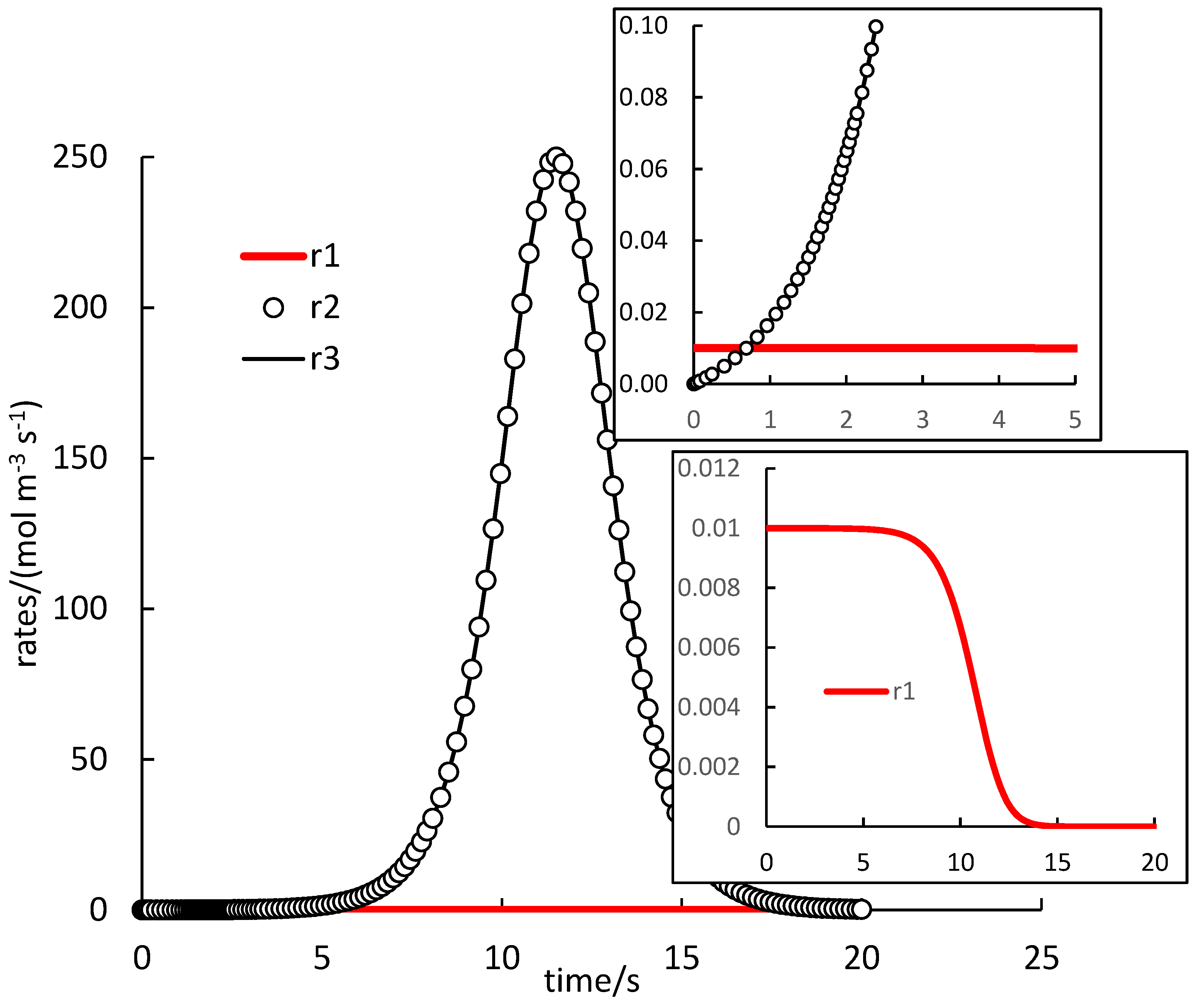
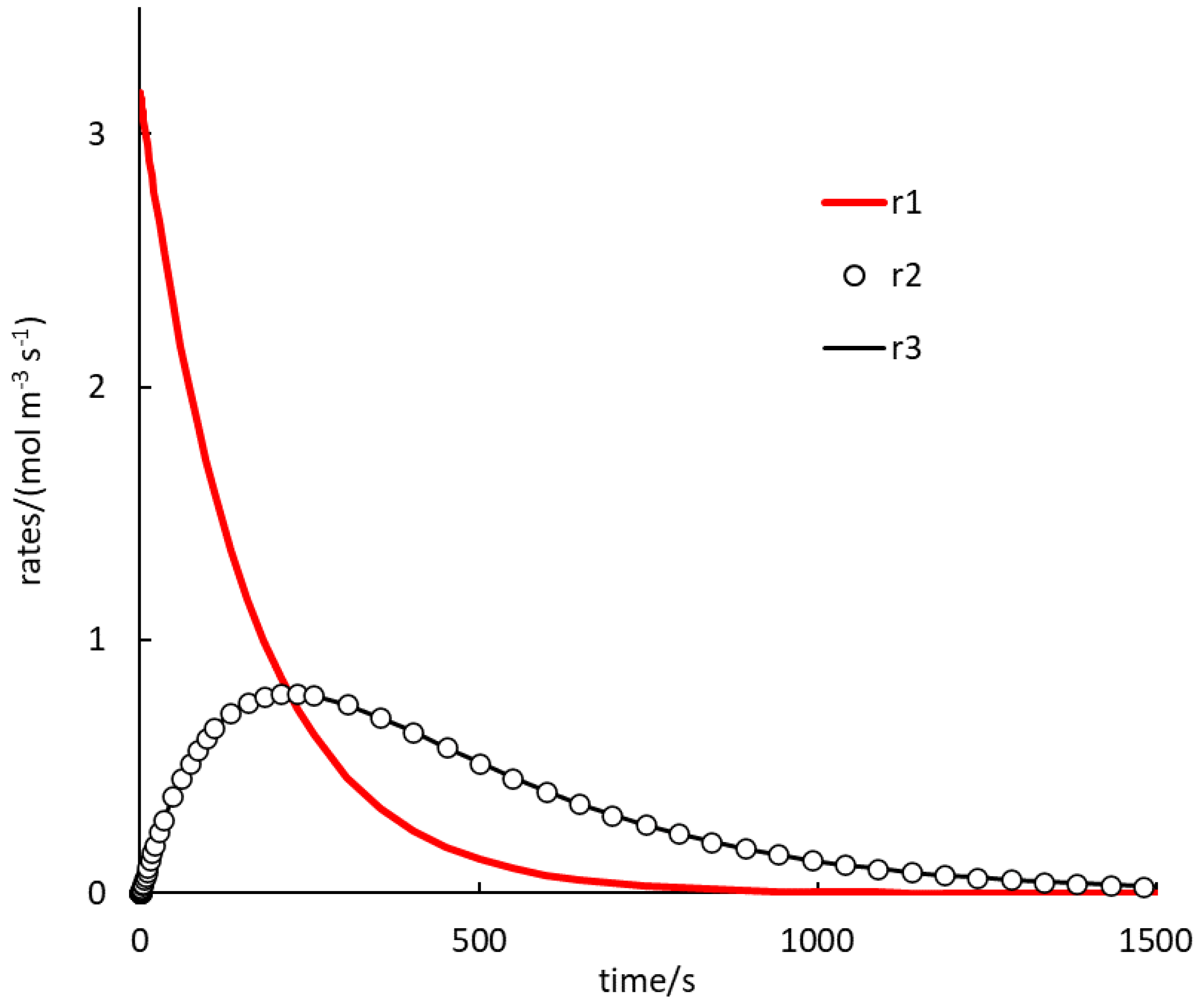
. Because autocatalysis is a kinetic phenomenon, it is very instructive to also inspect rate profiles. Two selected examples are shown in
Figure 1 and
Figure 2 (and they relate to the black and cyan curves in
Figure 1 of [
14], respectively). Both figures demonstrate the invalidity of the supposition that reaction (1.R3) is much faster than reactions (1.R1) and (1.R2), which was applied to select the values of
’s in ref. [
14]). This is the consequence of the fact that the reaction rate is affected not only by the value of its rate constant but also of the concentrations.
In
Figure 1, the rate of (1.R1) is very low, except in the very beginning, and rates of (1.R2) and (1.R3) are almost identical (the difference not seen in the figure). The autocatalytic effect is seen in the rapid increase of the rate of (1.R3), which evidently also controls the rate of (1.R2) and maintains it at high values. The effect is delayed in some induction period, the length of which can be estimated from the whole course as 5 s, or, at least, about 1 s when the rate of (1.R1) starts to be smaller than the other two rates. Once the supply of reactants is exhausted, all rates drop down to zero forming maxima on
and
profiles.
In
Figure 2, the rate of (1.R1) is the highest for a rather long time. Rates of (1.R2) and (1.R3) are, again, almost identical during the whole course. Here, no induction period is observed and the profiles of the (1.R2), (1.R3) rates seem to always be concave. The autocatalytic effect can be seen here in increasing rates of (1.R2), (1.R3), while the rate of (1.R1) decreases progressively.
Both figures report on profiles in a batch reactor. In a continuous stirred tank reactor, the situation is rather different and discussed in more detail in the
Supplementary Materials. Discussions of autocatalytic kinetics should therefore keep in mind the type of system and consider continuous inflow forcing in flow-through systems.
2.5. Empirical Rate Equation
As noted in ref. [
14], the rate equation for an autocatalytic reaction is sometimes expressed in an empirical form with an additional term containing the product concentration with positive order. For reaction (1.R1) this means the rate Equation
,
. The thermodynamic approach used in this work enables a formulation of a very similar equation. Considering only the reaction mixture of
and
with equilibrium constant
, the third degree approximating polynomial leads to the rate equation
For a sufficiently high equilibrium constant this equation can be modified to , which with gives the empirical form with .
Alternatively, Equation (16) can be rewritten in the form
which formulates the rate of
in terms of
rate traditional mass action expression but with a concentration (and temperature) dependent rate constant
(and no presumptions on the magnitude of the equilibrium constant). The autocatalytic effect is hidden in the concentration dependency of
.
2.6. Note on Diffusion
When chemical reactions are coupled with diffusion, concentration changes are not caused only by chemical transformations. This problem is outside the scope of this paper, and we add only a brief comparative note. Diffusion can be “self-balanced” which means a special restriction on diffusion fluxes, and it enables using the extent of reaction to describe concentration changes caused by reactions even in coupled reaction-diffusion systems [
22].
If the transformation of
to
occurs as a single reaction
, diffusion is self-balancing when
[
23]. The symbol
is explained in detail in ref. [
23] but here it is sufficient to state that it represents the divergence of the diffusion flux of the component
.
If the transformation proceeds including intermediate , i. e. according to (R2), diffusion is self-balancing only when the following condition is fulfilled: . Interestingly, there is no direct effect of the diffusion flux of the intermediate on the self-balancing diffusion condition. On the other hand, the condition was affected by its presence in the reacting mixture compared to the case when it is absent. Coupling chemical reactions with diffusion could be common in biological systems. This brief note shows that in a simple chemical transformation, diffusion fluxes can be affected differently due to the presence or absence of an intermediate involved in the autocatalytic scheme.


