Generalized Second Price Auctions over a Network

Abstract

We consider the problem of how to apply a generalized second price (GSP) auction to a buyer–seller network. GSP auctions are often used to sell online ads where buyers care about the position or placement of the ad. GSP auctions can also be applied to wireless data transmissions with congestion where buyers care about the speed of data transmission; however, such an auction would take place over a network as a buyer could only purchase from a seller (or cell tower) that he was linked to (or was close to). Two GSP auctions over a network are considered: separate GSP auctions, and integrated GSP auctions with pauses. The efficiency of these auctions is examined with efficiency favoring the integrated auction with pauses.

1. Introduction

Generalized second price (GSP) auctions are known for their use in online search advertising. Here, advertisers announce bids for keywords and then the ads are displayed in ranked positions where the advertiser who bids the most receives the top position and thus should receive the most clicks per ad. (For an empirical analysis of click through rates and the monetary value of a click, see Ghose and Yang [1]). These GSP auctions can be interpreted as taking place over a network where different advertisers are interested in (or linked to) different keyword-category searches. GSP auctions over a network can also be applied to the problem of radio spectrum pricing with congestion due to limited bandwidth; see Chen, Jana and Kannan [2]. Here, wireless consumers would submit a bid for cellular data and a cell tower would prioritize its transmission of data based on bids. Thus, the highest bidder would receive the fastest transmission of data. Wireless data transmission takes place over a network of consumers and cell phone towers where a consumer can only purchase a unit of data from a tower that he is close (or connected) to and such a consumer may be close (or connected) to multiple towers. As a final example, consider an auction for water where multiple farmers bid for water from different government-owned sources and the supply can be given on different days some of which are preferred to others because of the farming season; see Alevy, Cristi, and Melo [3]. However, due to location, not all farmers can receive water from all sources.

We consider the problem of how to apply a GSP auction to such a network framework and then examine auction efficiency. Two GSP auctions are considered over a network where a buyer can only enter a seller’s auction if the two are linked. The first considered is separate GSP auctions where each seller holds their own GSP auction and each buyer can enter only one auction even if such a buyer is linked to multiple sellers. (Buyers are assumed to be profit maximizers. For an analysis of GSP auctions where buyers can be value maximizers, see Wilkens, Cavallo, and Niazadeh [4]). We show that there exists a feasible assignment of buyers to sellers which respects the graph such that the separate auctions result in an efficient allocation of goods. However, if a buyer chooses to enter an auction where he does not displace another buyer instead of choosing an auction where he does displace another buyer, then the separate auctions may result in an inefficient allocation of goods.

The second auction considered is an integrated GSP auction with pauses. Here, each seller holds a separate auction and any buyers with links to multiple sellers participates in all of his linked seller’s auctions. Each auction is paused after the first multiple linked buyer reaches his drop out price (or maximum bid) which enables such a buyer to compare his final payoffs in each auction and then choose the one that gives him the highest payoff. (Note that if the auction with pauses were computerized, then each pause would occur quite briefly and thus would not disrupt service or slow the auction down). Auctions then continue and are paused again as the next multiple linked buyer reaches her drop out price. We show that such an auction has a unique equilibrium which is efficient.

There is a large and growing literature which examines generalized second price auctions and online advertising where advertisers care about the position that their ad is displayed in; see Varian [5], Varian and Harris [6], Edelman, Ostrovsky, and Schwarz [7], and Aggarwal, Goel, and Motwani [8]. Recent work has focused on efficiency of GSP auctions (see Gomes and Sweeney [9]), inefficiency under uncertainty (see Caragiannis, et al. [10]), as well as on seller’s revenue (see Yenmez [11]). For a model where some advertisers have limited information regarding the value of the display ads, see Arnosti, Beck, and Milgrom [12]. Athey and Ellison [13] consider auction design questions when advertising consumers search optimally. Lastly, competing ad auctions are modeled as Cournot-style competition in Ashlagi, Edelman, and Lee [14]. We add to this literature by allowing a GSP auction to occur over a network.

The current paper is also related to the market design literature and specifically to the auction design literature. For two recent surveys of this literature, see Abdulkadiroglu and Ausubel [15] and Loertscher, Marx, and Wilkening [16], and an overview of the issues addressed in this literature can be found in Klemperer [17]. The auction design literature is concerned with designing auctions that are implementable given the real-world context as well as designing auctions with desirable properties such as encouraging optimal allocation of goods. Our results are in the same vein as this genre since we are concerned with the efficiency of different GSP auctions over a network.

2. Model

Consider a generalized second price auction that takes place over a network.

Let $M=\{1,2,...,i,...,m\}$ represent the set of sellers and $N=\{1,2,...,j,...,n\}$ represent the number of buyers. Each seller i has $M_i=\{1,2,...,m_i\}$ goods for sale. The good in the set $M_i$ labeled k represents the kth position (or priority) of the goods i has available. In the case of radio spectrum, this priority represents the speed of data transmission where a cell tower gives priority to certain users who receive faster data transmission resulting in more data packets received in a given time. In the online search auction, the priority represents the ad’s position on the page where the top ranked ads receive more clicks per ad. In the water auction example, the priority represents the timing of the water received where farms prefer water at certain times.

A good in the position labeled 1 will have priority over other goods and will have the fastest data transmission or the most data packets received in a given time. The expected number of data packets received for a buyer whose good has priority k is $s_k$. If $k<k^{\prime }$, then $s_k>s_{k^{\prime }}$ for all $k\le m_i$ and $k^{\prime }\le m_i+1$. Assume that $s_k=0$ for all $k>m_i$.

The value of a data packet to buyer j is $v_j$. Buyer j’s payoff from receiving a good with priority k is $s_k·v_j$ minus the price paid. It is assumed that each $v_j$ is a random variable independently and identically distributed on $[\underline{v},\overline{v}]$ with continuous distribution F, where $\underline{v}\ge 0$. We assume that $v_j\ne v_{j^{\prime }}$ for all $j\ne j^{\prime }$. Additionally, we assume that buyer j would like to purchase at most one good (or one ad or one cell tower connection). Let $v\equiv \{v_1,v_2,...,v_n\}$.

Buyer j can purchase from seller i only if i and j are linked. We let g represent the set of links between sellers and buyers and G represents the set of all possible such graphs. Assume g consists of a single connected component. If there are multiple unconnected components, all analysis can be done separately. Let $ij\in g$ represent a link between i and j. In the radio spectrum example, this network represents connections between cell phone customers and cell towers where customers can only purchase data from towers they are physically close to. Note that we assume for simplicity that each customer wants to purchase data from at most one cell tower; thus, if a cell phone customer is in the proximity of multiple towers and so has multiple network ties, then he may participate in two or more auctions, but he only wants to purchase data from the tower that offers him the best deal. In the online search example, the network is made up of links between keywords and advertisers where a link is only present if an advertiser wants to place an ad in a particular keyword search.

An allocation $A\left(g\right)$ of goods is feasible in network g if (i) each buyer j receives at most one good; if the good received has priority k and is from seller i, then it must be that $ij\in g$ and if (ii) each seller i sells at most one good with priority $k\le m_i$. Let $\widehat{A}\left(g\right)$ represent the set of all feasible allocations over g.

An allocation $A^{*}\left(g\right)\in \widehat{A}\left(g\right)$ is efficient if $A^{*}\left(g\right)$ solves $ma{x}_{A\left(g\right)\in \widehat{A}\left(g\right)}{\sum }_{j=1}^n{s}_{k_j^{A\left(g\right)}}·v_j$ where $k_j^{A\left(g\right)}$ is the priority j is assigned in allocation $A\left(g\right)$. Thus, we assume that the seller does not consume the good if there is no sale.

Let the social welfare of allocation $A\left(g\right)$ be $S{W}_{A\left(g\right)}={\sum }_{j=1}^n{s}_{k_j^{A\left(g\right)}}·v_j$. Thus, an efficient allocation maximizes social welfare.

We consider two possible generalized second price (GSP) ascending-bid auctions: separate auctions and integrated auctions with pauses. These auctions are based on the GSP ascending-bid auction of Edelman, Ostrovsky, and Schwarz [7].

In the separate auctions, each seller holds his own GSP ascending-bid auction and buyers linked to multiple sellers can choose one auction to compete in. This choice results in a feasible assignment of buyers to sellers in graph g. Thus, there would be m GSP ascending-bid auctions. In seller i’s auction, the buyers with the top $m_i$ bids would receive a good. As in Edelman, Ostrovsky, and Schwarz [7], the price in seller i’s auction starts at zero and rises with a clock. Each buyer then decides when to drop out. Let buyer j drop out at bid $b_j$. Let $b_{\left(j\right)}$ denote the bid (or drop out price) of the jth highest bidder, let $n\left(j\right)$ denote the identity of this bidder, and let $v_{\left(j\right)}$ denote his valuation. The auction ends when there is only one bidder left. Let this top bidder $n\left(1\right)$ receive the good with priority position 1 and let him pay $s_1·b_{\left(2\right)}$. The awarding of goods continues in this fashion; thus, a buyer who drops out at bid $b_{\left(j\right)}$ would receive a good with priority position j and would pay price $s_j·b_{(j+1)}$; if there is no agent $(j+1),$ then set price $b_{(j+1)}=0$. Let any bidders who do not receive a good pay price 0. Let the number of bidders participating in seller i’s auction be $n_i$.

The second auction we consider is the integrated auction with pauses. The goods are auctioned off in separate auctions where at first any buyer with links to multiple sellers participates in all of his linked seller’s auctions. Auctions will be paused so that the buyers with multiple links can compare payoffs across auctions and use this information to drop out of low payoff auctions. Specifically, pause each auction after the multiple linked buyer with the lowest drop out price reaches this price. Keep these auctions paused until any other auction with multiple linked buyers is paused; if there is an auction with no multiple linked bidders, then this auction will not pause. Let any buyer who has announced drop out bids in all of his linked sellers’ auctions compare his final payoffs in each auction and keep the highest such payoff. Assign this buyer to the auction with the highest payoff and remove him from the other auctions; if there is a tie for the highest payoff assign the buyer randomly to one of the corresponding auctions. If there is a paused auction where no buyer has dropped out, then keep this auction paused. Let all paused auctions with a buyer who has dropped out continue until the multiple linked buyer with the next lowest drop out price reaches this price. When all auctions with remaining multiple linked bidders are paused, let any buyer who has announced drop out bids in all of his auctions compare his payoffs and remove him from the auctions with the lowest payoffs. Continue this process until all multiple linked bidders have been assigned to only one auction. Let all auctions continue. Assign prices and goods as in the separate auctions case.

Remark 1.

Next, we discuss the motivation in selecting the separate auctions and the integrated auction with pauses. The separate auctions are chosen as they are the simplest way to extend the GSP auctions to a network environment, and they would be fairly easy to implement. For instance, in the radio spectrum example, the separate auctions are perhaps the most straightforward way to extend the spectrum auction of Chen, Jana and Kannan [2] to a network of towers and cell phone owners. The integrated auctions with pauses were selected as a way to extend the auction used in Kranton and Minehart [18] to a GSP framework; the Kranton and Minehart [18] auction is quite desirable as it provides a way to efficiently allocate goods over a network. However, in Kranton and Minehart [18], the goods auctioned off are all identical and there are no differences in priorities. In a GSP framework, items are not identical and it matters which seller a buyer purchases from because different sellers can give the same buyer a different priority. Thus, in order to achieve efficiency, we need to let a buyer compare what he would get from different sellers, whereas, in Kranton and Minehart [18], this comparison is not necessary as all sellers give a buyer the same payoff. The integrated auction with pauses is a natural way to let a buyer discover on his own which auction is best in an ascending bid framework.

3. Results

3.1. Separate GSP Auctions

We compare the efficiency of the auctions starting with the separate GSP auctions. For this auction, we first establish the existence of an equilibrium given that each buyer has already decided which of his connected seller’s auctions he will participate in. This Lemma is based on Theorem 2 of Edelman, Ostrovsky, and Schwarz [7], which assumes a single seller with $n_i=m_i+1$.

Lemma 1.

In each separate auction, there is a unique Bayes–Nash equilibrium where a buyer j who receives a good with priority position k will drop out of the auction at price $b_j=v_j-\frac{s_k}{s_{k-1}}(v_j-b_{(k+1)})$ for all $n\left(j\right)<m_i$ and for $n\left(j\right)=m_i$ when $n_i>m_i$. In all other cases, $b_j=v_j$. Any buyer j such that $n\left(j\right)\le m_i$ receives the good and $n\left(j\right)$ receives priority position j; any buyer for which $n\left(j\right)>m_i$ does not receive a good.

All proofs can be found in the Appendx Appendix A.

Lemma 1 shows the existence of a unique equilibrium in each separate auction and provides the maximum bid a buyer will place (called the drop out bid). Notice that the agent with the largest valuation will stay in the auction the longest and will win the top priority position.

Next, we consider the efficiency of the separate GSP auctions. First, we show by Proposition 1 that there exists an efficient separate auction equilibrium. In Propositions 2 and 3, we give conditions under which the separate auction B-N equilibrium is inefficient, which is the result of an incorrect assignment of buyers to sellers’ auctions. If only one assignment of buyers to seller’s auctions is efficient and if the number of sellers is large, then most equilibria will be inefficient.

Proposition 1.

There exists a feasible assignment of buyers to sellers in graph g such that the Bayes–Nash equilibrium of the separate auctions results in an efficient allocation of goods.

Proposition 1 ensures that there exists a separate auction equilibrium which is efficient. To see this, note that, in a given efficient allocation of goods, each buyer purchases from one particular seller. An efficient equilibrium is achieved in the separate auctions game, if each buyer is placed in his “correct” seller’s auction. Notice that if only one allocation is efficient and if there are many buyers and sellers, then it should be unlikely that each buyer is assigned to the correct auction. Although efficiency is always possible, it may be difficult to achieve in the separate auctions case.

Consider a buyer j with links to multiple sellers in g. Let all buyers in g have already decided which auctions to participate in except for buyer j. We say that j displaces $j^{\prime }$ if $ij,i{j}^{\prime }\in g$ and if $j^{\prime }$ would win a unit in i’s auction if j does not participate in this auction and $j^{\prime }$ would not win a unit in i’s auction if j does participate in the auction.

Proposition 2.

Let there exist a buyer j with multiple links in graph g and let all other buyers have already decided which auctions to participate in. Assume $m_i<n_i$ for all $i\in M$. Assume if j chooses to participate in $\widehat{i}$’s auction, then j displaces another buyer but j does not displace a buyer if he chooses any other auction. If j does not participate in $\widehat{i}$’s auction, the resulting B-N equilibrium of the separate auctions will result in an inefficient allocation of goods.

Proposition 2 gives conditions under which the separate auctions result in an inefficient equilibrium. Specifically, Proposition 2 considers the case where all items are sold. Here, efficiency requires that a buyer join an auction where he displaces another buyer rather than join an auction where he does not displace a buyer. If a buyer displaces another buyer, then, by Lemma 1, he must value the good more than the other bidders and efficiency requires that he ends up with the good, while if a buyer does not displace another buyer then he must value the good less and there is no efficiency gain from him joining this auction.

Proposition 3.

Let there exist a buyer j with multiple seller links such that j displaces another buyer if he participates in any of these separate auctions. Assume that all other buyers have already decided efficiently which auctions to participate in. The resulting B-N equilibrium allocation will be efficient for j joining at least one seller’s auction and will be inefficient for j joining the remaining auctions.

Proposition 3 also gives conditions under which the separate auctions result in an inefficient equilibrium. Proposition 3 assumes that there is a buyer who always displaces another buyer no matter which auction he chooses. Efficiency requires that he choose the auction that will maximize social welfare, otherwise the resulting equilibrium will be inefficient. If the number of such sellers is large, then again it should be unlikely that efficiency is achieved.

Note that we assumed in Proposition 3 that all other buyers have already made the efficient choice of which auction to participate in. We could instead assume that some of these buyers had chosen to participate in an auction such that the resulting B-N equilibrium allocation would not be efficient regardless of j’s choice. Then, buyer j’s choice of which auction to join would still affect social welfare given the choices already made by the other buyers. It would still be the case that j’s joining at least one seller’s auction would maximize social welfare given the constraint of the choices made by the other buyers and joining any other auctions would not.

We consider an environment where a buyer is not able to accurately estimate which auction would be best and thus a buyer chooses which auction to participate in at random or with limited information. In the radio spectrum example, a cell phone customer may not know which other customers are currently in the proximity of a given tower and so does not know what his payoff would be from participating in a given auction.

Next, we formalize this by incorporating random first-stage assignments of auction participation into our analysis. Define the two-stage separate auction game as follows. In the first stage, each buyer randomly chooses to participate in one of his linked seller’s auctions. In the second stage, the separate auctions take place as described in Section 2.

Corollary 1.

In the two-stage separate auction game, there is a positive probability that the separate auctions results in an efficient allocation of goods.

Corollary 2.

In the two-stage separate auction game, let there be a buyer j with multiple seller links such that j displaces another buyer if he participates in any of these separate auctions. There is a positive probability that the separate auctions results in an inefficient allocation of goods.

These corollaries follow directly from Propositions 1 and 3.

Note that one could extend this analysis to the repeated game case which would allow buyers to learn information regarding past payoffs from different sellers or auctions. Buyers could then use past payoffs to guide their decision of which auction to participate in. However, in such a repeated game, one would expect for the network to change over time which would make the analysis quite complex. For instance, in the radio spectrum example, buyers would continually change locations and so past payoff success may not guarantee future payoff success. For simplicity, we consider a fixed network and a one-shot game. Additional discussion of such a repeated game can be found in the conclusion.

Remark 2.

In Corollaries 1 and 2, buyers randomly decide which seller’s auction to participate in. Alternatively, one could allow buyers to choose sellers by best responding to the choices of other buyers. Here, each buyer would have full information about everything except for other buyers’ valuations. Instead, each buyer would simply know the distribution from which other buyers’ valuations were drawn from. One could then ask if inefficient equilibria resist to reasonable equilibrium selection criteria. Example 1 below illustrates that in fact such inefficient equilibria would resist reasonable equilibrium selection criteria. In this example, there is one buyer who is linked to two different sellers. Each seller has the same number of goods for sale and the same number of additional buyer links. Thus, a priori there is no way for the multiple linked buyers to distinguish between the two sellers. Thus, if he is given the opportunity to choose which seller he will purchase from, he can do no better than to choose at random. However, such a random choice would be inefficient half of the time as, given the other buyers actual valuations, one auction is clearly more efficient for him to participate in. Thus, the separate auctions do not provide the buyer with the information needed to make an efficient choice.

The following example illustrates Proposition 3 and Corollary 2.

Example 1.

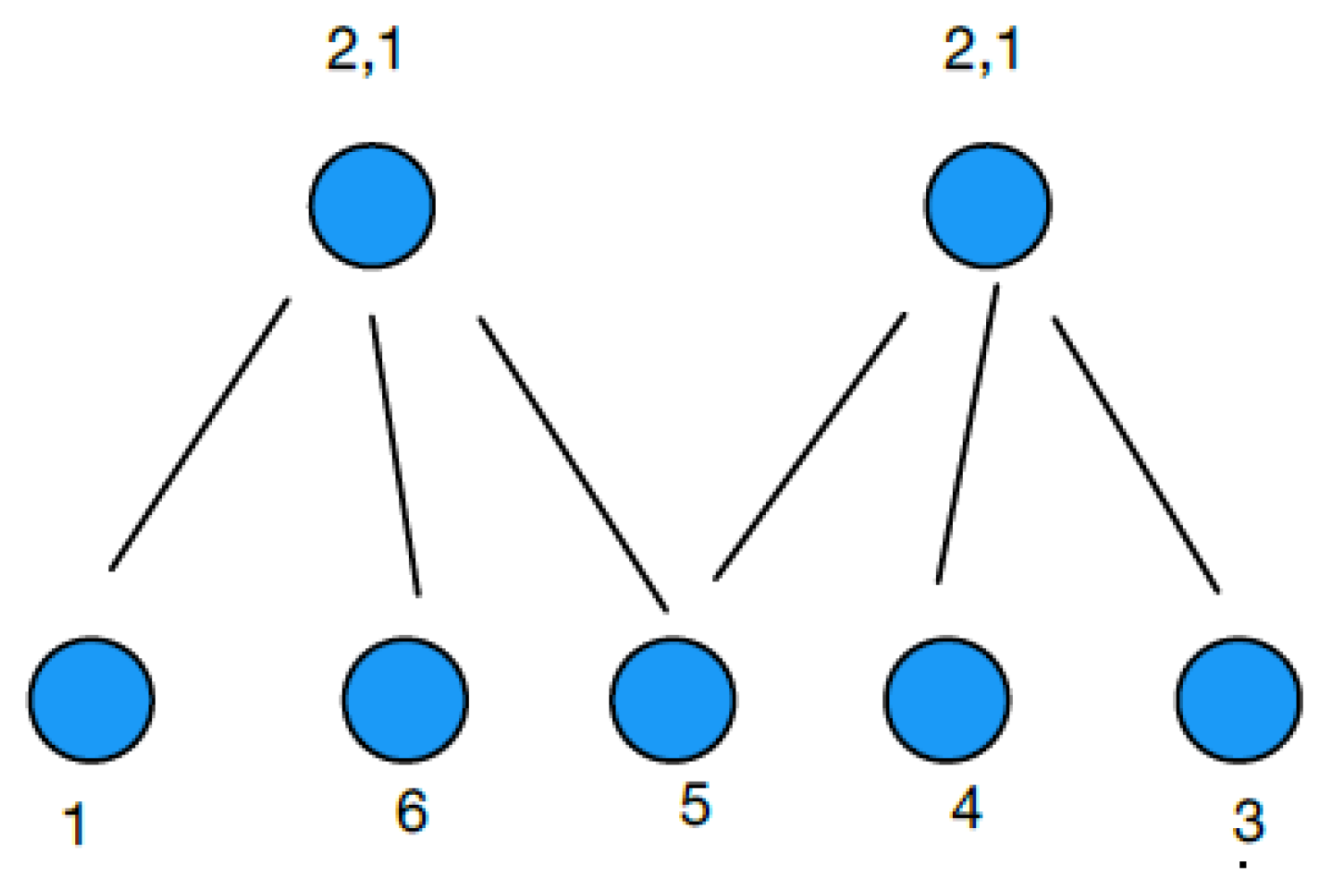
Let $M=\{1,2\}$, $N=\{1,2,3,4,5\}$, $v=\{1,6,5,4,3\}$, $M_i=\{2,2\}$, $s_1=2$, $s_2=1$, and $g=\{11,12,13,23,24,25\}$; this graph is represented by Figure 1. In Figure 1, the nodes and numbers on the bottom represent buyers and their corresponding valuations. The nodes and numbers on the top represent sellers and the $s_1$, $s_2$ values; both $s_1$ and $s_2$ appear above each seller as each has two goods for sale which are of two different priorities.

Efficiency requires that buyer 3 participate in seller 1’s auction. Such an allocation results in the sum of the payoffs to all buyers and sellers equal to $6·2+5·1+4·2+3·1=28$, while, if 3 chooses seller 2’s auction, the sum of payoffs equals 27. Here, if 3 chooses seller 1’s auction, then he displaces buyer 1 who has quite a low valuation while, if 3 chooses seller 2’s auction, then he displaces buyer 5 whose valuation is much higher. Thus, it would only be efficient if he chooses auction 1.

3.2. Integrated Auction with Pauses

Next, we consider the integrated auction with pauses and show that its unique Bayes–Nash equilibrium allocation is efficient. We assume here that $s_k·v_j$ is unique for all k and j.

Proposition 4.

In the integrated auction with pauses, there is a unique Bayes–Nash equilibrium in bids.

In the integrated auction with pauses, buyers with multiple links will participate in all of their linked sellers’ auctions. These buyers will eventually have their auctions paused at their corresponding drop out prices or bids. These buyers can then choose to participate in the auction which is best. As we have assumed that $s_k·v_j$ is unique, this choice will also be unique as will be the corresponding bids, thus resulting in a unique Bayes–Nash equilibrium.

Proposition 5.

The Bayes–Nash equilibrium of the integrated auction with pauses is efficient.

The proof proceeds by induction showing that if all other buyers have made the efficient decision, then the buyer with the highest valuation will also make the correct decision of which auction to participate in when his auctions are paused at his drop out prices. Inductively, the buyer with the second highest valuation will also have incentive to make the correct or efficient decision of which auction to join. Thus, the integrated auction with pauses has an efficient equilibrium.

Next, we consider an example in which one buyer is linked to or in range of two different sellers and efficiency requires that he buy from the second seller which will result in not all goods being sold. If the buyer makes such a decision randomly, then efficiency will result only half of the time. However, we show that the equilibrium of the integrated auction with pauses is efficient.

Example 2.

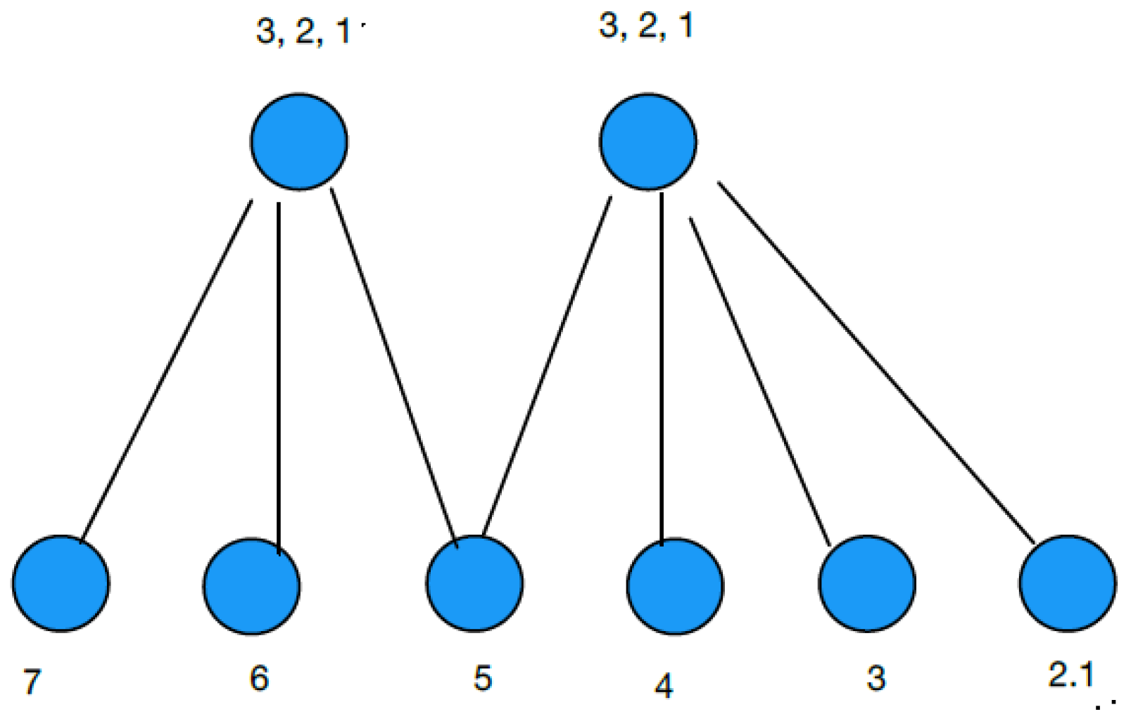
Let $M=\{1,2\}$, $N=\{1,2,3,4,5,6\}$, $v=\{7,6,5,4,3,2.1\}$, $M_i=\{3,3\}$, $s_1=3$, $s_2=2$, $s_3=1$, and $g=\{11,12,13,23,24,25,26\}$; see Figure 2. In this graph, buyer 3 can buy from either seller 1 or 2. However, it is efficient for buyer 3 to buy from seller 2 and thus not all of the goods will be sold. To see this, we sum up the buyers’ valuations. If buyer 3 purchases from seller 1, then the buyer with the highest valuation is assigned the top priority from each seller and this results in a sum of buyers’ valuations of $S{W}_1=3\times 7+2\times 6+1\times 5+3\times 4+2\times 3+1\times 2.1=58.1$. If instead buyer 3 purchases from seller 2, then the sum of the buyers’ valuations is $S{W}_2=3\times 7+2\times 6+3\times 5+2\times 4+1\times 3=59.$ Even though seller 1 is unable to sell his last unit, the sum of the payoffs is highest when buyer 3 purchases from seller 2 and is able to receive the top priority for the good.

Consider the integrated auction with pauses. Here, the two auctions will take place separately with buyer 3 bidding in both and with both auctions paused at his corresponding drop out bids. Bidder 3 will then compare his payoff in the two auctions. In 1’s auction, $b_3^1=2.5$ and $u_3^1=5$. In 2’s auction, buyer 4 will drop out at price $4-\frac{2}{3}(4-2.55)=3.03$. Thus, 3’s drop out price in this auction is $b_3^2>3.03$ with corresponding payoff $3(5-3.03)=5.91$. Thus, bidder 3 will choose to participate in 2’s auction, which is efficient.

Remark 3.

We determine which auctions are efficient when people have limited information ahead of time about others. For instance, a buyer may not know or have a good estimate of how many other buyers are linked to each seller and also may not know or have a good estimate of what these other buyers’ valuations are. In the wireless data example, people frequently change locations and so a buyer may not be able to accurately estimate which other buyers are in a given cell tower’s range and may not be able to accurately estimate auction payoffs in advance.

When information is limited, the integrated auction with pauses seems to be the best auction if efficiency is the main goal; Proposition 5 shows that this auction’s equilibrium is efficient. Note that this auction does not require a buyer to have information ahead of time, but rather a multiple linked buyer will learn during the auction’s pauses which seller’s auction is best to remain in. Alternatively, in the separate auctions case, a buyer with limited information will not know or learn which auction is best. Such a buyer is likely to make his decision of which auction to participate in randomly, and the resulting equilibrium may be inefficient as shown in Propositions 2 and 3.

4. Conclusions

We compared the efficiency of GSP auctions over a network. Results showed that the separate auctions are unlikely to be efficient unless multiple-linked agents are able to correctly forecast which auctions to join. However, the integrated auction with pauses has a unique equilibrium which is efficient as agents have full information about link payoffs when they decide which auction to compete in.

An interesting extension of this model would be to allow the auction game to be repeated while additionally allowing buyers to form and sever ties to sellers; such network changes could result from a buyer changing locations in the radio spectrum example. Thus, each period, the network would be slightly different and each period an auction would take place. One could then determine which networks players are more likely to spend time in.

Additionally, agents with multiple ties the previous period could have a preference for a previous seller’s auction if they received a high enough payoff. One could then analyze how such a preference for the previous seller’s auction influences the efficiency of the equilibrium. For instance, in the separate auctions case, a buyer with multiple links could learn which seller’s auctions on average gave him a higher payoff and could then be more likely to choose to participate in these auctions in the future. This choice could increase the likelihood of efficiency in the separate auctions.

References

- Ghose, A.; Yang, S. An empirical analysis of search engine advertising: Sponsored search in electronic markets. Manag. Sci. 2009, 55, 1605–1622. [Google Scholar] [CrossRef]
- Chen, Y.F.; Jana, R.; Kannan, K.N. Using generalized second price auction for congestion pricing. In Proceedings of the 2011 IEEE Global Telecommunications Conference, Houston, TX, USA, 5–9 December 2011. [Google Scholar]
- Alevy, J.E.; Cristi, O.; Melo, O. Right-to-choose auctions: A field study of water markets in the Limari Valley of Chile. Agric. Res. Econ. Rev. 2010, 39, 213–226. [Google Scholar] [CrossRef]
- Wilkens, C.A.; Cavallo, R.; Niazadeh, R. GSP: The Cinderella of Mechanism Design. In Proceedings of the 26th International Conference on World Wide Web Conferences Steering Committee, Perth, Australia, 3–7 April 2017. [Google Scholar]
- Varian, H.R. Position auctions. Int. J. Ind. Organ. 2007, 25, 1163–1178. [Google Scholar] [CrossRef]
- Varian, H.R.; Harris, C. The VCG auction in theory and practice. Am. Econ. Rev. 2014, 104, 442–445. [Google Scholar] [CrossRef]
- Edelman, E.; Ostrovsky, M.; Schwarz, M. Internet advertising and the generalized second-price auction: Selling billions of dollars worth of keywords. Am. Econ. Rev. 2007, 97, 242–259. [Google Scholar] [CrossRef]
- Aggarwal, G.; Goel, A.; Motwani, R. Truthful auctions for pricing search keywords. In Proceedings of the 7th ACM Conference on Electronic Commerce, Ann Arbor, MI, USA, 11–15 June 2006. [Google Scholar]
- Gomes, R.; Sweeney, K. Bayes–Nash equilibria of the generalized second-price auction. Games Econ. Behav. 2014, 86, 421–437. [Google Scholar] [CrossRef]
- Caragiannis, I.; Kaklamanis, C.; Kanellopoulos, P.; Kyropoulou, M.; Lucier, B.; Leme, R.P.; Tardos, E. Bounding the inefficiency of outcomes in generalized second price auctions. J. Econ. Theory 2015, 156, 343–388. [Google Scholar] [CrossRef]
- Yenmez, M.B. Pricing in position auctions and online advertising. Econ. Theory 2014, 55, 243–256. [Google Scholar] [CrossRef]
- Arnosti, N.; Beck, M.; Milgrom, P. Adverse Selection and Auction Design for Internet Display Advertising. Am. Econ. Rev. 2016, 106, 2852–2866. [Google Scholar] [CrossRef]
- Athey, S.; Ellison, G. Position auctions with consumer search. Q. J. Econ. 2011, 126, 1213–1270. [Google Scholar] [CrossRef]
- Ashlagi, I.; Edelman, B.G.; Lee, H.S. Competing ad Auctions; Harvard Business School: Boston, MA, USA, 2013. [Google Scholar]
- Abdulkadiroglu, A.; Ausubel, L.M. Market Design. 2016. Available online: http://www.ausubel.com/econ704/Abdulkadiroglu-Ausubel-Market-Design-Survey.pdf (accessed on 9 July 2018).
- Loertscher, S.; Marx, L.M.; Wilkening, T. A Long Way Coming: Designing Centralized Markets with Privately Informed Buyers and Sellers. J. Econ. Lit. 2015, 53, 857–897. [Google Scholar] [CrossRef]
- Klemperer, P. What really matters in auction design. J. Econ. Perspect. 2002, 16, 169–189. [Google Scholar] [CrossRef]
- Kranton, R.E.; Minehart, D.F. A Theory of Buyer-Seller Networks. Am. Econ. Rev. 2001, 91, 485–508. [Google Scholar] [CrossRef]
Figure 1.
Buyer–seller graph.
Figure 2.
© 2018 by the author. Licensee MDPI, Basel, Switzerland. This article is an open access article distributed under the terms and conditions of the Creative Commons Attribution (CC BY) license (http://creativecommons.org/licenses/by/4.0/).
Share and Cite
MDPI and ACS Style
Watts, A. Generalized Second Price Auctions over a Network. Games 2018, 9, 67. https://doi.org/10.3390/g9030067
AMA Style
Watts A. Generalized Second Price Auctions over a Network. Games. 2018; 9(3):67. https://doi.org/10.3390/g9030067
Chicago/Turabian StyleWatts, Alison. 2018. "Generalized Second Price Auctions over a Network" Games 9, no. 3: 67. https://doi.org/10.3390/g9030067
APA StyleWatts, A. (2018). Generalized Second Price Auctions over a Network. Games, 9(3), 67. https://doi.org/10.3390/g9030067
Note that from the first issue of 2016, this journal uses article numbers instead of page numbers. See further details here.