1. Introduction
Biological species (viruses, bacteria, insects, plants, or animals) develop, compete, reproduce, and evolve. Different species have different evolutionary strategies, some fail to survive while others are selected [
1]. The evolution of biological species can be modeled mathematically as an evolutionary game, with the equilibrium strategies of the game as prediction for the ultimate distributions of species in population, when some species may survive with positive proportion, while others become extinct [
2,
3]. We say a strategy is dense if it contains a large and diverse number of positive species, and is sparse if it has only a few dominant ones.
Assume that populations may have mixed strategies, or in other words, assume that they are a polymorphic mixture of pure strategists. Let
be the strategy vector of a subpopulation, with
being the frequency or chance of the subpopulation to be species
i,
. Let
be the composition profile of the population, with
being the fraction of species
j,
. The average payoff for a subpopulation of strategy
x in population of composition
y would be
, where
is the payoff of the subpopulation of species
i in population of species
j, and
is called the payoff matrix [
4,
5,
6].
For an evolutionary game, a composition
is defined to be an equilibrium of the game, when the payoff of any subpopulation with the same strategy
is maximized:
where
is the set of all possible strategies [
4,
5,
6].
John Nash (1950, 1951) [
7,
8] showed that for an
n-person non-cooperative game, there always exists an equilibrium strategy, now called Nash equilibrium bearing his name. However, computing an equilibrium strategy is hard in general. In fact, many types of games are proved to be NP-hard in terms of their computational complexities [
9,
10,
11,
12]. An evolutionary game is also NP-hard. For example, the evolutionary game on a graph, with the adjacency matrix of the graph as the payoff matrix, is equivalent to a maximum clique problem, which is NP-complete [
13,
14,
15].
Many algorithms have been developed for computing equilibrium strategies of games, most notable, the Shapley-Snow algorithm [
16], the Lemke-Howson algorithm [
17], and the quadratic programming algorithm by Mangasarian and Stone [
18]. The Shapley-Snow algorithm searches strategies with all possible numbers of nonzero components and reports all equilibrium ones. The Lemke-Howson algorithm follows a procedure similar to the simplex algorithm for linear programming along a special path of strategies that hopefully leads to an equilibrium strategy. The quadratic programming algorithm tries to find a strategy that satisfies a set of complementarity conditions necessary and sufficient for equilibrium strategies by solving a specially constructed quadratic program. The Lemke-Howson algorithm and the quadratic programming algorithm are efficient if they succeed, but they can only find one equilibrium strategy, which cannot be prescribed. The Shapley-Snow algorithm is more expensive, but can in principle find all possible equilibrium strategies.
We are interested in computing the equilibrium strategies of a given evolutionary game and in particular, the strategies with a sparse or dense set of nonzero components. The Shapley-Snow algorithm is thus a natural choice of the algorithm, for it can be modified straightforwardly to find the sparsest or densest equilibrium strategy, as we will describe in greater detail in the rest of the paper, while the Lemke-Howson algorithm and the quadratic programming algorithm cannot be modified easily to serve our purpose.
The problem of computing sparse or dense equilibrium strategies is challenging yet interesting both computationally and practically. Similar problems have been investigated in other closely related fields such as in regularization of least squares regression [
19,
20] and in signal reconstruction in compressive sensing [
21,
22,
23,
24]. In both cases, a sparse solution is sought for the problem by minimizing the
-norm of the solution. These studies have many applications in science and engineering, and have made great impacts in broad areas of scientific computing.
Computing sparse or dense equilibrium strategies is of great computational challenge, because the computation of such a strategy can be computationally very expensive when the problem size is large: Since the equilibrium strategies do not form a continuous set of strategies, there is no regularization schemes such as the -norm minimization for least-squares regression and compressive sensing that can be used to obtain a sparse or dense equilibrium strategy. A general algorithm such as the Shapley-Snow algorithm has to be adopted with certain modifications. Yet, in the worst case, the computation time may still grow exponentially with increasing problem size.
Computing sparse or dense equilibrium strategies is of great interest in biological and social applications. For example, in ecological modeling, to preserve biodiversity, it is important to predict a population state with only a few species left or with most species kept in population [
1,
25]. In economic analysis, to optimize investment portfolio, it is crucial to know more risky investment plans when the funds are concentrated to only a few stocks or more balanced plans when the funds are more diversified. The portfolio optimization problem can be formulated as an evolutionary game with the sparsest equilibrium strategy corresponding to the most risky investment plan, and the densest one to the most balanced plan [
26,
27].
In this paper, we show that the equilibrium strategies of an evolutionary game, including sparse and dense ones, can be computed by implementing a standard Shapley-Snow algorithm. We then show that by using a modified Shapley-Snow algorithm, sparse equilibrium strategies for an evolutionary game can be computed relatively easily, while dense ones are much more computationally costly. However, we show that by formulating a “complementary” problem for the computation of equilibrium strategies, we can reduce the cost for computing dense equilibrium strategies and obtain them much more efficiently. We describe the primary and complementary algorithms and present test results on randomly generated games as well as a game related to allele selection in genetic studies. In particular, we demonstrate that the complementary algorithm is about an order of magnitude faster than the primary algorithm to obtain the dense equilibrium strategies for all our test cases.
Note that in biology, the diversity of a given population can be measured by the richness of species types and the evenness of species distribution. The richness of species in population
x can be represented by the number of nonzero elements of
x. The evenness of species can be measured with different standards [
25]. In this paper, we will only check the standard deviation of nonzero elements of
x for the evenness of species, for the focus of this study is on computation not biological analysis.
where
.
3. Dense vs. Sparse Equilibria
The Shapley-Snow algorithm described in the previous section computes the equilibrium strategies of all possible sizes of p for a given evolutionary game. We therefore call it a Complete Shapley-Snow Algorithm. In this algorithm, the equilibrium strategies are computed in the order of increasing sizes of p, i.e., first, strategies with the smallest number of positive components, and then larger ones, and the largest in the end. Therefore, the algorithm can be modified easily to find only a sparse or dense equilibrium, say a strategy with the smallest or largest number of positive components. The following Algorithms 2 and 3 are the algorithms that can be implemented for such purposes.
| Algorithm 2: A Sparse Shapley-Snow Algorithm |
For do
For each do
If is nonsingular and then
,
End
If and then
is a Nash equilibrium, record , exit.
End
End
End |
| Algorithm 3: A Dense Shapley-Snow Algorithm |
For do
For each do
If is nonsingular and then
,
End
If and then
is a Nash equilibrium, record , exit.
End
End
End |
In Algorithm 2, the Sparse Shapley-Snow Algorithm, the strategies with small numbers of positive components are examined first. The algorithm exits once an equilibrium strategy with the smallest number of positive components is found. In Algorithm 3, the Dense Shapley-Snow Algorithm, the strategies with large numbers of positive components are examined first. It exits after an equilibrium strategy with the largest number of positive components is found. The former only solves some small linear systems of equations and does not require much computation, while the latter needs to solve relatively large linear systems and is more computationally expensive.
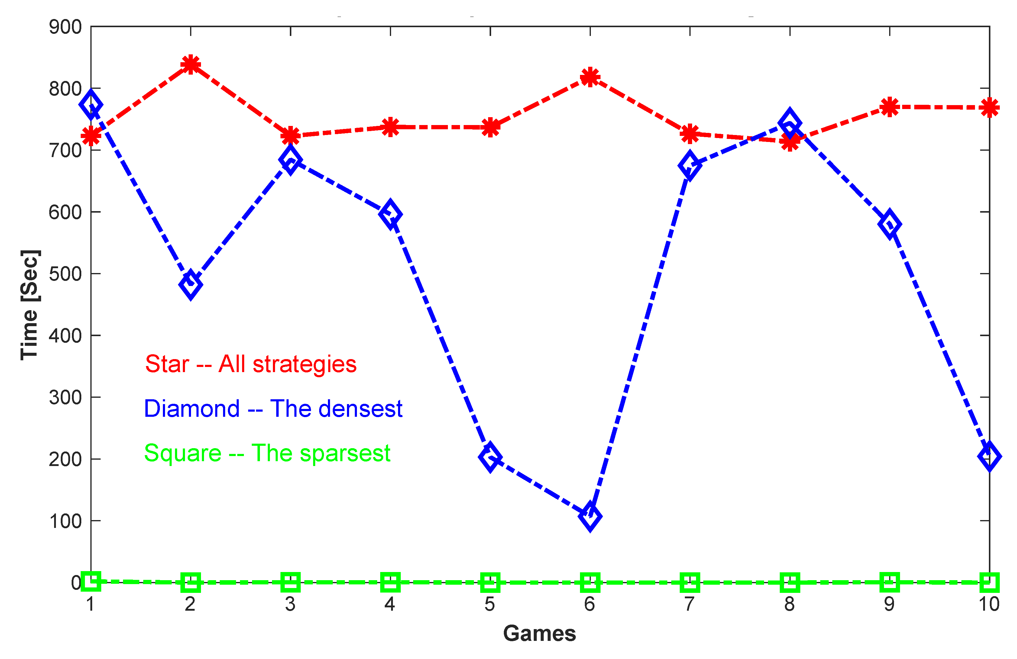
We have implemented the complete, sparse, and dense versions of the Shapley-Snow algorithm in Matlab on a 1.3 GHz MacBook Air, and tested them on a randomly generated set of evolutionary games. A total of 10 games are generated, each having 20 strategies and defined by a 20 by 20 randomly generated payoff matrix, i.e., all the entries of the matrix are set to a random number in between 0 and 1. The reason to test a set of randomly generated games is to avoid possible biases from specially structured games, and instead to have a relatively broad range of test cases in terms of numbers, sparsities, and densities of their equilibrium strategies.
From
Table 1, we see that by using Algorithm 1, the Complete Shapley-Snow Algorithm, all equilibrium strategies are found for each of the games. The total number of equilibrium strategies for each game ranges from 9 to 65. However, the time spent to find all the strategies for each game is relatively long, and is about the same for all the games, in between 700 and 800 s. This is because the algorithm needs to exhaust all possible trial strategies, from those with 1 positive component, to those with 2, 3, …,
n. No matter how many equilibrium strategies are there for each game, the amount of work required to find them all is about the same.
Table 2 shows the results for computing the sparsest equilibrium strategies for the tested games. Since the Sparse Shapley-Snow Algorithm exits immediately once it finds the equilibrium strategy of the smallest number of positive components, the algorithm does not require much computation time. Therefore, the sparser the first equilibrium strategy, the shorter the required computation time. Indeed, all the cases where there is only 1 positive component in the sparsest equilibrium take only 0.02 s to finish; The time is increased for the case where there are 2 positive components; and most cases where there are 3 positive components require about 0.44 s except for 1 case which takes 1.83 s. In general, the amount of computation required to find the sparsest equilibrium strategy is small because the algorithm only solves a set of small linear systems of equations before it finds the first and also the sparsest equilibrium strategy.
Table 3 is the opposite of
Table 2. It shows the results for computing the densest equilibrium strategies of the tested games. Since the Dense Shapley-Snow Algorithm starts with the strategies with the largest number of positive components, it is much more time consuming because it requires the solution of many relatively large linear systems before it finds the first and densest equilibrium strategy. Therefore, the denser the first equilibrium strategy, the less time consuming to find it. As shown in
Table 3, the densest equilibrium strategy found for Game 6 has 14 positive components, and requires 107.01 s, while the densest equilibrium strategy found for Game 1 has 6 positive components and requires 773.53 s. In general, computing the densest equilibrium strategy seems much more expensive than computing the sparsest one. Note also that in
Table 2 and
Table 3, we have listed the average values and standard deviations of the positive components of the strategies. It seems that the standard deviations are in the same order of the corresponding average values. Therefore, the positive components seem unevenly distributed. However, since the games are only randomly generated and our focus is on the performance of the algorithms, we will not further discuss the richness and evenness of these strategies.
Figure 1 shows a more direct comparison in computation time for computing all the equilibrium strategies, or only the sparsest, or only the densest for all the test cases.
4. Complementary Formulation of Evolutionary Games
Consider the necessary and sufficient conditions in (
4).
which can be called a primary set of conditions. Let
. Assume that
A is nonsingular. Then,
. Let
. We can then obtain a so-called complementary set of conditions:
Since
, we call
a primary equilibrium strategy and
a complementary.
Note that the conditions in (
9) are equivalent to
where
is the
ith row of matrix
B.
Let
and
and
. Then, based on the conditions in (
10),
for all
. The latter can be written in a more compact form as
, where
, and
. Since
,
. It follows that
and
must satisfy the following equations.
In addition,
for all
, which can be simplified to
where
.
Since
, we can derive
from
if we can find
using the conditions in (
11) and (
12). However, in order to find
, we do not have the prior knowledge on
q. Therefore, we need to enumerate all possible set of indices
q, to see if any gives rise to a complementary equilibrium strategy
. Once
is found, we can recover
immediately. We call this procedure a Complementary Shapley-Snow Algorithm. Let
be the set of all subsets of
of size
k. Assume that
. Then, the algorithm can be described formally as Algorithm 4.
Note that when a complementary equilibrium strategy is found, , , and . It follows that , and is a corresponding primary equilibrium strategy of positive components. Thus, as all the possible sizes of q are enumerated in Algorithm 4, the Complete Complementary Shapley-Snow Algorithm, all the possible complementary equilibrium strategies can be found with and , and hence are all the possible primary equilibrium strategies with and .
| Algorithm 4: A Complete Complementary Shapley-Snow Algorithm |
For do
For each do
If is nonsingular then
,
.
End
If and then
is a complementary equilibrium strategy.
End
End
End |
5. Computing Dense Equilibria in Complementary Forms
Similar to the primary Shapley-Snow algorithm, the complete version of the complementary algorithm can be modified to compute the sparse as well as dense complementary equilibrium strategies of a given game. Assume that A is nonsingular. Let . In addition, assume that . We then have the Algorithms 5 and 6:
| Algorithm 5: A Sparse Complementary Shapley-Snow Algorithm |
For do
For each do
If is nonsingular then
,
.
End
If and then
is a complementary equilibrium strategy, exit.
End
End
End |
| Algorithm 6: A Dense Complementary Shapley-Snow Algorithm |
For do
For each do
If is nonsingular then
,
.
End
If and then
is a complementary equilibrium strategy, exit.
End
End
End |
Let
and
be a pair of primary and complementary equilibrium strategies. Since
and
are complementary to each other, if
is the sparsest primary equilibrium strategy,
must be the densest among all complementary equilibrium strategies. Similarly, if
is the densest,
must be the sparsest. As we have discussed in previous sections, dense equilibrium strategies can be computationally more costly than the sparse ones. Therefore, they may be computed more efficiently through their complementary strategies, which are sparse. In particular, the densest primary equilibrium strategy
may be computed through the corresponding complementary strategy
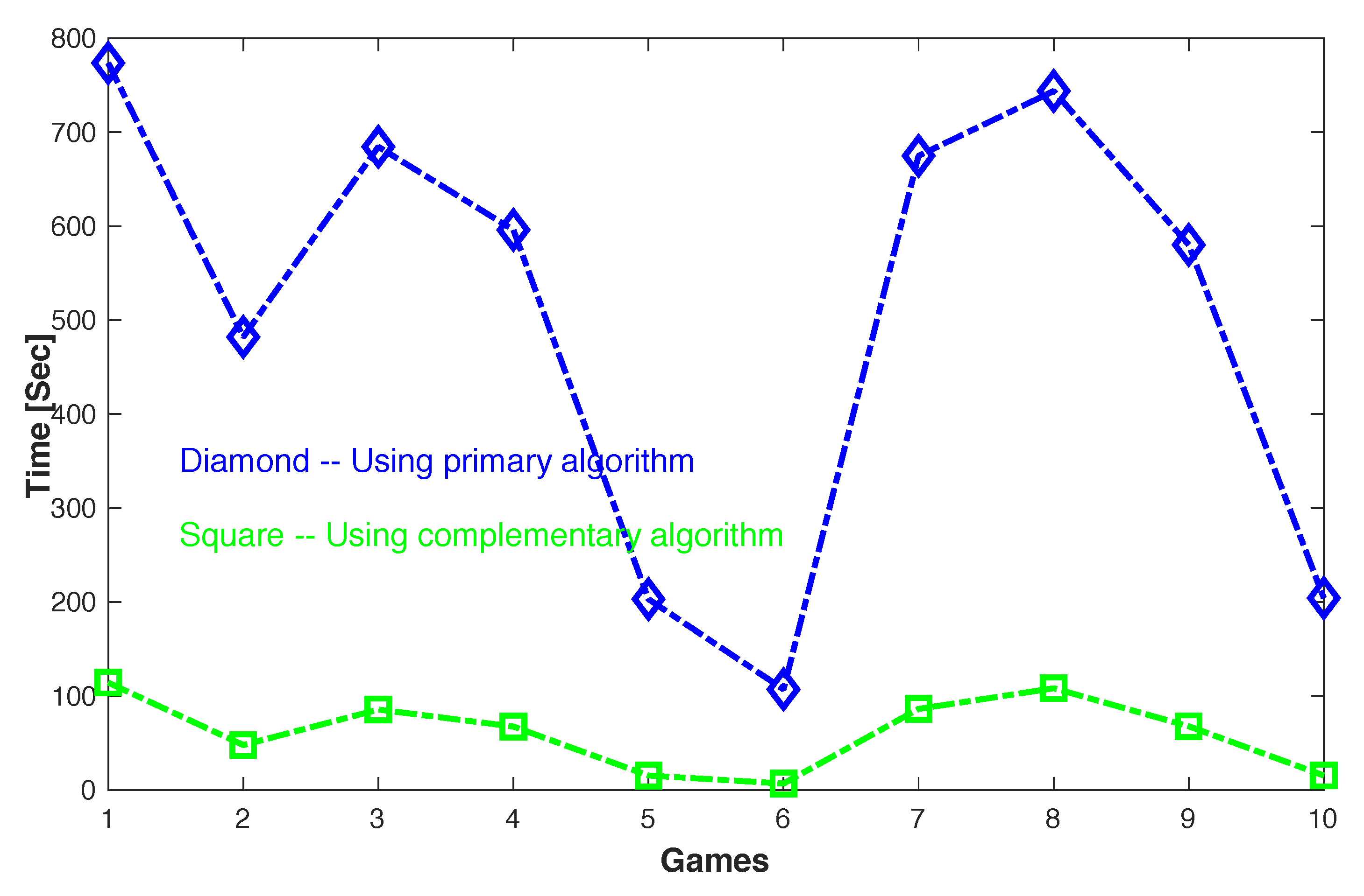
. The latter is the sparsest among all complementary equilibrium strategies and can be found efficiently using Algorithm 5, the Sparse Complementary Shapley-Snow Algorithm. Indeed, as we can see in
Table 4, the time for computing the densest equilibrium strategy
using Algorithm 3, the primary dense Shapley-Snow algorithm is much longer than that for computing the corresponding complementary strategy
using Algorithm 5, the sparse complementary Shapley-Snow algorithm. More specifically, the computation time is reduced by 7 to 15 times in 10 tested games. Note that the 10 tested games are the same randomly generated ones as shown in
Table 1,
Table 2 and
Table 3.
Figure 2 displays a more direct comparison between the primary and complementary algorithms for computing the densest equilibrium strategies of these games.
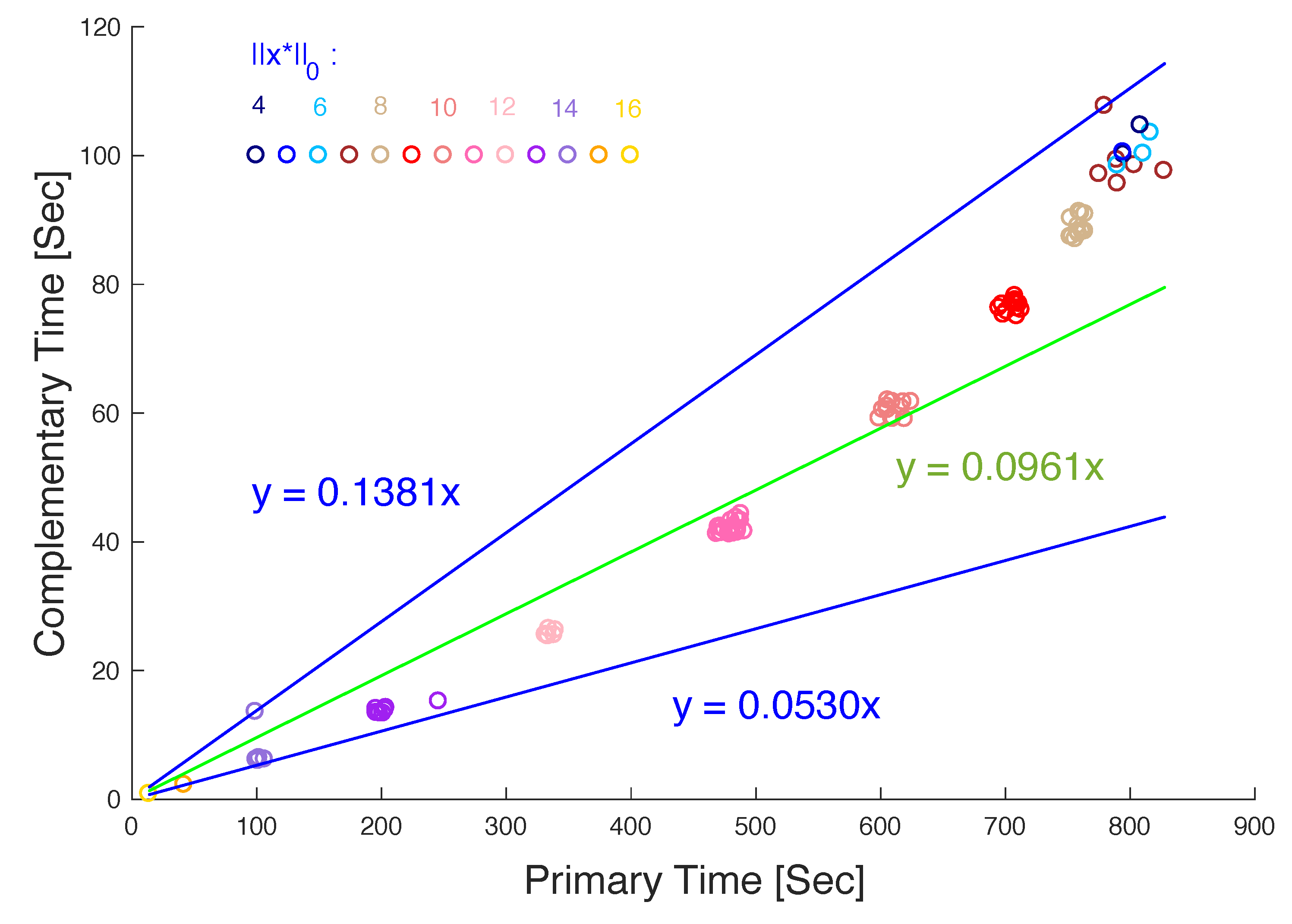
In order to obtain more statistical assessments, we have also tested the primary and complementary Shapley-Snow algorithms, i.e., Algorithm 3 and Algorithm 5, for computing the densest equilibrium strategies for an additional 100 randomly generated games, each again with 20 strategies. The results further confirm that the complementary algorithm outperforms the primary algorithm for all the test cases. More specifically, the average time required by the primary algorithm is 519.98 s, while the time by the complementary algorithm is only 53.88 s, about an order of magnitude faster.
Figure 3 shows more detailed comparisons between the two algorithms. Note that the time required by both algorithms varies for different games, depending on the density of the densest equilibrium strategy of the game, but the relative difference in time between the two algorithms remains about the same: In
Figure 3, the x-axis corresponds to the time used by the primary algorithm, while the y-axis to that by the complementary algorithm. Each circle in the graph corresponds to the times required by the primary and complementary algorithms for one of the tested games. The density of the densest strategies found ranges from 4 to 16 and is color coded on the circles: The density, i.e., the richness or more specifically, the number of nonzero components of the strategy, denoted as
, increases in the order of 4, 5, 6, 7, 8, 9, 10, 11, 12, 13, 14, 15, 16, as the color of the circle changes in the order of dark blue, blue, light blue, brown, light brown, red, light red, pink, light pink, purple, light purple, orange, light orange, respectively. Note that all the circles are above the line
and below
, showing that the computation time by the complementary algorithm can be as small as 5.3 percent of the time by the primary algorithm, and at most 13.81 percent. In average, the former is about 9.61 percent of the latter, as indicated by the median line
. Note also that in general, for both algorithms, the lower the density of the densest equilibrium strategy found, the longer the computation time. For the primary algorithm, this is because more relatively large systems need to be solved if the density of the densest strategy is lower. For the complementary algorithm, it means that the density of the corresponding complementary strategy is higher, which also requires the solution of more systems, although beginning with relatively small ones.
Finally, as a special case, we have also tested a game related to allele selection in genetic studies [
5,
28,
29,
30,
31,
32]. Assume that there are
n alleles at a given genetic locus. Let
be a selection strategy for the alleles, with
being the allele frequency for allele
i. Let
be a graph representing allele matching, where
is a set of nodes corresponding to the alleles, and
E is a set of links between the nodes. If allele
i and
j can make a successful genotype, then there is a link between node
i and
j. Then, an evolutionary game can be defined for allele selection with the adjacency matrix
A for graph
G as the payoff matrix, where
for all
i,
for all
and
, and
for
and
.
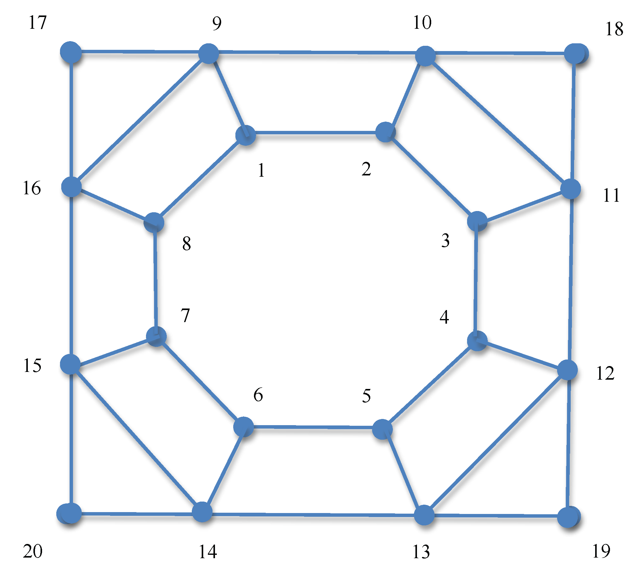
We have considered an allele selection game with
, i.e., 20 alleles and
A being the adjacency matrix for the graph shown in
Figure 4. It is easy to verify that for this game,
, with
for
and
for
, is an equilibrium strategy, as it satisfies all the necessary and sufficient conditions for equilibrium strategies as stated in (
4). It turns out that
is also the densest equilibrium strategy for this game. We have thus applied both primary (dense) and (sparse) complementary Shapley-Snow algorithms to compute the densest equilibrium strategy for this game and recorded the computing times. Our results showed that both algorithms recovered the densest equilibrium strategy
accurately. However, the complementary Shapley-Snow took only
s in three runs, while the primary Shapley Snow required
s, respectively, again suggesting that the complementary algorithm can be more or less an order of magnitude more efficient than the primary one for computing the densest equilibrium strategy for a game.
Note that in all our test cases, we should be able to obtain the same set of equilibrium strategies for each game using either primary or complementary algorithms, including the sparsest and densest ones. In other words, if we obtain a set of equilibrium strategies for a given game using the primary algorithm, we should be able to obtain all the corresponding complementary strategies using the complementary algorithm. In this way, we can obtain from all found by the complementary algorithm the same set of equilibrium strategies found by the primary algorithm, and vice versa. Otherwise, the sparsest equilibrium strategy found in the primary dense algorithm may not necessarily be found in the sparse complementary algorithm, if the latter cannot find the corresponding complementary strategy . This property is important, but is not so obviously shown in the descriptions of the algorithms. We therefore provide a more formal verification in the following.
As required by the algorithms, we assume that payoff matrix A is nonsingular. Let . We then show that for each equilibrium strategy with positive components that is found by the primary Shapley-Snow algorithm, a corresponding complementary strategy with and can be found by the complementary Shapley-Snow algorithm, where , and . Note that in the primary algorithm, an equilibrium strategy with positive components is found if is nonsingular and . On the other hand, the corresponding complementary strategy with and is obtained by the complementary algorithm if is nonsingular and , where . Therefore, all we need to show is that for the given pair of p and q, is nonsingular and if and only if is nonsingular and , which follows immediately from the following two theorems.
Theorem 1. Let p and q be two subsets of indices, and . Assume that A is nonsingular. Then, is nonsingular if and only if is nonsingular, where and .
Proof. If
is nonsingular, then
is a Shur’s complement of
A [
33]. Since
A is nonsingular,
. It follows that
and
is nonsingular. Since
,
is nonsingular. Reversely, if
is nonsingular, then
is a Shur’s complement of
B. Since
B is nonsingular,
. It follows that
and
is nonsingular. Since
,
is nonsingular. ☐
Theorem 2. Let A be a payoff matrix. Assume that A is nonsingular, , and . Let . Then, is nonsingular if and only if is nonsingular and .
Proof. If
, it suffices to show that
is nonsingular if and only if
is nonsingular and
.
Let
and
. Then
By Sherman-Morrison-Woodbery Formula [
33],
is nonsinglar if and only if
is nonsingular and
. In addition,
By Theorem 1,
is nonsingular if and only if
is nonsingular. In addition,
Since
is a Shur’s complement of
B,
. But
. Therefore,
and
It follows that if and only if . ☐
Again, an equilibrium strategy can be found in either the primary algorithm under the conditions is nonsingular and or in the complementary algorithm with its complementary strategy under the conditions is nonsingular and . Based on the above two theorems, the two sets of conditions are equivalent and therefore, can indeed be found by either algorithm, and so is .
6. Concluding Remarks
In this paper, we have considered the problem of computing the equilibrium strategies of a given evolutionary game, complete, sparse, or dense. We are particularly interested in computing the dense equilibrium strategies, for they may represent more diverse ecological conditions in biology or more even distributions of funds in financial investment. If such system states can be determined, further analysis on related properties such as the stabilities of the states and their dynamic behaviors may provide great insights into maintaining the diversities of the system and preventing certain species from extinction. In any case, the dense equilibrium strategies are more costly to compute than the sparse ones as we have demonstrated in the paper. We have therefore formulated a complementary version of the game for a given primary one, and shown that computing a dense strategy for the primary version then becomes computing a sparse strategy in the complementary version, which can be done much more efficiently.
We have implemented the primary and complementary Shapley-Snow algorithms in Matlab for all the complete, sparse, and dense versions. We have tested these algorithms on randomly generated games and analyzed their performance. In particular, we have shown that the complementary algorithm is on average about 10 times faster than the primary algorithm for finding the densest equilibrium strategies for the given games. We have also particularly tested a more realistic game related to allele selection in genetic studies. The results on this game are consistent with those for randomly generated games: The computing time to find the densest equilibrium strategy for the game using the complementary algorithm is more or less an order of magnitude more efficient than using the primary algorithm.
In our algorithms, the conditions under which a primary equilibrium strategy
is found are different from those under which the corresponding complementary equilibrium strategy
is found. Therefore, it is not clear if
can always be found by the complementary algorithm given
found by the primary algorithm, and vice versa. In other words, if a set of equilibrium strategies
is obtained using the primary algorithm, it is not clear if all the corresponding complementary strategies
can be found using the complementary algorithm, and vice versa. In any case, in the end of
Section 5, we have provided a formal justification showing that the two sets of conditions are equivalent, and the two algorithms should be able to produce and only produce all the corresponding equilibrium strategies. Note that for our complementary algorithms to work, we did assume the payoff matrix
A to be nonsingular, which will limit to some extent the applicability of the algorithms.
The focus of this paper is on computation and especially on computation of dense equilibrium strategies. Many related issues have not yet been addressed. For example, we have only concerned ourselves with the richness of the strategies but not with the evenness, which can be important in practice. Further development of algorithms that can find both rich and even equilibrium strategies can be interesting. In economic application, the payoff of a strategy may correspond to the risk of investment. The higher the payoff, the lower the risk. Therefore, it would be interesting to find not only a dense strategy but also a dense strategy with the highest possible payoff. Then, a more extensive search for such a strategy may be required in the current algorithms. Finally, we have not considered the evolutionary stability of equilibrium strategies, either sparse or dense, while it is of great concern in both biological and economic applications. We will investigate how to compute sparse and dense equilibrium strategies efficiently while at the same time justifying their stabilities in our future research efforts.


