1. Introduction
The minimum effort game, also known as the weak link game, is a stylized way to model the production of any good whose output depends on the weakest component of production. Many goods have this property and so the game has been widely applied over the last thirty years or so. For example, it has been used to look at the provision of public goods (Hirschleifer 1983 [
1]), performance within organizations (Knez and Camerer 1994 [
2], Brandts and Cooper 2006 [
3]) and performance within nations (Bryant 1983 [
4], Cooper and John 1988 [
5]). The game is also the subject of a large experimental literature that has primarily focused on the difficulties of achieving coordination on the Pareto efficient outcome (e.g., Van Huyck, Battalio and Beil 1990 [
6], Devetag and Ortmann 2007 [
7]).
The key issue in the minimum effort game is that of equilibrium selection (Van Huyck et al. 1990 [
6]). The Pareto efficient outcome is for every player to choose highest effort, and, crucially, unlike a linear public good game (or prisoners dilemma), this outcome is a Nash equilibrium. Specifically, it is individually rational for a player to choose high effort if all others also chose high effort. Choosing high effort is, however, ‘risky’ because it only takes one player to choose low effort for this costly effort to have been wasted. Play often, therefore, converges on the inefficient equilibrium in which everyone chooses low effort (Camerer 2003 [
8]), although there are exceptions (e.g., Engelmann and Normann 2010 [
9]).
The equilibrium selection issue means the minimum effort game is of interest for, at least two distinct reasons. First, from an applied perspective it gives us crucial insight on the difficulties of maintaining cooperation in small groups. As such, it provides an ideal test-bed for interventions that can potentially increase cooperation (e.g., Chaudhuri and Paichayontvijit 2010 [
10]). Second, from a theoretical perspective the minimum effort game provides a simple and tractable setting with which to test theories of equilibrium selection and learning in games (e.g., Monderer and Shapley 1996 [
11], Anderson, Goeree and Holt 2001 [
12], Crawford 2001 [
13], Goerg, Neugebauer and Sadrieh 2016 [
14]).
Given the importance of the minimum effort game it is crucial to understand individual incentives within the game as completely as possible. The current paper adds to that understanding with two related results—one on the set of equilibria and a second on the optimal strategy as a function of beliefs.
The set of pure strategy Nash equilibria in the minimum effort game is trivial and well known. Anderson et al. (2001) [
12] detail the set of symmetric mixed strategy Nash equilibria in a game with a continuum of actions (see their Appendix). In the current paper we fully characterize the set of mixed strategy Nash equilibria in games with a finite action set. It is shown (Theorem 1) that such equilibria take a very particular form: they are
symmetric, involve players randomizing over
two actions, and the probability of choosing an action depends solely on the
cost benefit ratio and the
number of players. From a technical point of view, the main value added of our result is to show that all equilibria are symmetric.
Theorem 1 is not a surprise given the analysis of Anderson et al. (2001) [
12]. We provide, however, an independent proof which we argue can provide additional insight. In particular, our second main result (Theorem 2) provides a general expression for the optimal strategy in the minimum effort game. This expression maps from a player’s beliefs to an optimal strategy and provides a very specific trade-off between optimal effort, the number of players and the cost benefit ratio. To put this result in context we highlight that surprisingly little is known about how changes in the costs and benefits of effort translate into behavior in the minimum effort game. This is a fundamental gap in our understanding. We argue that our results provide a framework around which this issue can be explored in more detail. Arguing this point makes more sense after stating the results and so we return to this issue in
Section 4.
We proceed as follows:
Section 2 introduces the minimum effort game,
Section 3 details the set of equilibria,
Section 4 details the optimal strategy and applications.
Section 5 concludes.
3. Nash Equilibria in the Minimum Effort Game
We begin with a useful lemma. In order to state the result more succinctly we introduce some notation. Given any player
, strategy
, and effort level
, let
denote the probability player
i will choose an effort level of
k or above. Given any player
, strategy profile
, and effort level
, let
In interpretation
is the probability that the minimum effort level chosen by players other than
i will be
k or above.
Lemma 1. Consider any player , strategy profile σ and effort level , Proof. For any effort level
, let
Let
. Please note that
is the probability the minimum effort level chosen by players other than
i will be
k. Consider any effort level
k where
. The expected payoff of player
i if she chooses effort level
k can be written
The expected payoff of player
i if she chooses effort level
can be written
1From Equations (
5) and (
6) we get
for all
. The statement of the Lemma follows immediately. ☐
Lemma 1 provides the key ingredient with which to derive the set of Nash equilibria. This set is detailed in our next result. Part (i) of this result is trivial and not new. Part (ii) is analogous to the result of Anderson et al. (2001) [
12] for games with a continuous actions set but our method of proof is different. Technically, the method of Anderson et al. (2001) [
12] focuses on symmetric equilibria. We show that all equilibria are symmetric and so close that possible loophole.
Theorem 1. Strategy profile is a Nash equilibrium of the weak link game if and only if either:
- (i)
There exists effort level such that - (ii)
There exist effort levels , where , such that
Proof. We take as given a Nash equilibrium . Please note that, by definition, for all i and . Also, . These observations leave us with three possibilities to consider.
Case 1. Suppose that there exists some player and effort level such that and .
Recursively applying relation (
4) we see that
for any
. Similarly, we see that
for any
. Given that
is a Nash equilibrium, this implies that
. Consider any player
. That
implies
. Applying relation (
4) we know
for any
. Hence,
for all
. By definition, therefore, (see Equation (
3))
Using
gives
. Applying relation (
4) we see that
for any
. Hence,
. Given that player
j was chosen without loss of generality we can see that
for all
, as given in part (i) of the statement of the Theorem.
Case 2. Suppose that there exists some player
such that
. This is a minor variant on case 1. Applying relation (
4) we see that
for any
. Thus,
. Consider any player
. By definition
Using
gives
. Applying relation (
4) we see that
for any
. Hence,
. Given that player
j was chosen without loss of generality we know that
for all
, as given in part (i) of the statement of the Theorem.
Case 3. For every player there exists a non-empty set of actions such that for every (and for every ).
Consider any player
. Let
. We know
for any
. Thus,
for any
. This implies that
for any
and any
. So,
. Given, however, that players
i and
j were chosen without loss of generality we obtain
for all
. Moreover, we know
for all
. We also know,
. Thus,
for all
. Let
. Given that
we know
.
For every player
let
. Select a player
i for which
for all
. Let
. Given that
it must be that
for all
and
. By assumption,
for all
and
. Thus, applying relation (
4), we know that
for all
and
. Putting this together tells us that
for all
and
. Thus,
for all
. If
then
and
giving a contradiction. Thus,
. Applying Lemma 1, it must be that
for all
. So, repeating the previous arguments, we get
for all
, and
.
To summarize, we know that
and
for all
. We also know that
for all
. Putting this together gives
We obtain an equilibrium as given in part (ii) of the statement of the Theorem. It is clear that
can take any plausible values, where
. ☐
Theorem 1 part (i) demonstrates that there are
K pure strategy Nash equilibria and part (ii) demonstrates that there are
mixed strategy equilibria. This gives a total of
equilibria in the minimum effort game. The three most immediate properties of the Nash equilibria are: (a) all of the equilibria are symmetric, (b) at most two effort levels are chosen with positive probability, and (c) the equilibrium probability of choosing an effort level depends solely on the cost benefit ratio and the number of players (and is independent of the effort level). As Anderson et al. (2001) [
12] point out these three properties have some interesting implications that are worth briefly exploring. To focus the discussion, for any
where
, denote by
the Nash equilibrium strategy profile
where
for all
i, and by
the profile where
.
An important implication of properties (a) and (b), and particularly of symmetry, is that we can easily Pareto rank the set of Nash equilibria. It is well known that the pure strategy Nash equilibria of the weak link game are Pareto ranked (Van Huyck, Battalio and Beil 1990 [
6]). Indeed, this is one of the main reasons that the weak link game has been much studied. Theorem 1 implies that all the Nash equilibria are Pareto ranked. Specifically, given equilibrium
the minimum effort level is clearly
k. Hence,
for all
. Given equilibrium
we know (see the proof of Theorem 1) that any player
is indifferent between choosing effort level
l and effort level
k. If they choose effort level
l then the minimum effort level is
l. Hence
for all
and any
. Thus, equilibria can be Pareto ranked by ‘lowest’ effort level.
For any there are Nash equilibria with expected payoff . The higher the expected payoff, therefore, the fewer Nash equilibria with that expected payoff. While the expected payoff is determined solely by the lowest effort level, l, it is worth appreciating that the realized payoff may depend on the higher effort level, k. Specifically, the payoff of player i if he chooses effort level k will be either or . Thus, the difference between minimum and maximum possible realized payoff is increasing in the difference between l and k. We can, thus, rank equilibria in terms of expected payoff and ‘risk’.
Consider the comparative statics of equilibrium
. Anderson et al. (2001) [
12] highlight the counter-intuitive property that an increase in
leads to an increase in the probability of the higher effort level
k. Another counter-intuitive property concerns the number of players
n. The larger is
n then the larger is the equilibrium probability of choosing the higher effort level. Indeed, as
we have
. So, individual behavior ‘converges’ on a pure strategy equilibrium. Crucially, however, equilibrium payoffs do
not change with
n and are equal to
. To understand this better we need to look at aggregate behavior. The probability with which a player
i can expect to coordinate with others does not depend on
n
Hence an increase in
n does not change expected payoffs. The probability of all players coordinating on high effort is increasing with
n but converges to
Aggregate behavior, therefore, does not converge on a pure strategy equilibrium.
The counter-intuitive properties discussed above follow, in a technical sense, from the need to keep a player indifferent between choosing the low and high effort levels l and k. The payoff from the lowest effort level is fixed at and so if, say, the benefit from coordinating on high effort is reduced the probability of coordinating on high effort needs to increase to compensate. Hence we see an increased equilibrium probability of each player choosing high effort. This illustrates that incentives to choose high effort are driven by the number of players and the cost benefit ratio. In the following section we pick this up and move beyond equilibrium analysis.
4. Beliefs and Optimal Effort
Recall that the equilibrium probability of choosing an effort level depends solely on the cost benefit ratio and the number of players. With this in mind, consider, for a given
, the equilibria
. For each of these equilibria, the probability with which player
i chooses effort level
k is the same. This suggests that player
i’s incentives to choose
k does not depend on what effort level other players might be choosing, as long as it is less than
k.
2 This allows us to say something about the optimal effort level of a player, even if play is not consistent with Nash equilibrium. We will frame this result as a mapping from a player’s ‘beliefs about others’ to an optimal effort level. This framing seems pertinent given the focus on beliefs in the previous literature (Crawford 1995 [
15], Crawford and Broseta 1998 [
16], Crawford 2001 [
13], Costa-Gomes, Crawford and Iriberri 2009 [
17]).
For every player , assume that there is a function where is the probability player i puts on a player choosing effort level k. For example, if then player i expects each of the other players to independently choose effort 1 with probability . Implicitly, this assumes that player i expects the actions of others to be uncorrelated and symmetric. These assumptions are very natural in the experimental lab where interaction is independent and anonymous. Function will be referred to as the beliefs of player i. It will be assumed for all i. For any, , let denote the probability that player i puts on a player choosing effort level k or less.
Given the beliefs of a player we can calculate his expected payoff. With a slight abuse of notation denote by the expected payoff of player i if he chooses effort level k and his beliefs are given by . Please note that if strategy profile satisfies for all and then . In general, however, player i’s beliefs may not correspond to the actual behavior of other players. The following result derives the optimal effort level of a player given his beliefs and is the second main result of the paper.
Theorem 2. Consider any player . If denotes the beliefs of player i andthen for all . Proof. With a slight abuse of notation, for all
let
denote the probability with which player
i believes the minimum choice of others will be
k or above. Set
. If strategy profile
satisfies
for all
then
. This allows us to apply Lemma 1.
Consider any
. By construction
3
Thus, using Equation (
10),
Please note that setting
we also get
Applying (
4) we see that
for all
. Consider next any
. By construction
Thus,
Applying (
4) we see that
for all
. Thus,
for all
. ☐
Theorem 2 provides a very simple way to work out the optimal effort level of a player given her beliefs. It also allows us, given the observed effort level of a player, to infer something about what her beliefs must have been. Unsurprisingly, we see that the optimal effort level is increasing in the benefit of effort
b and decreasing in the cost of effort
c and the number of players
n. More interesting is that we obtain a precise prediction of the trade-off between the benefit cost ratio and the number of players. This is something that can be applied in the experimental lab. Before we discuss that there is one important point to clarify about Theorem 2. This result applies to a one-shot game. If the game is repeated then a player may potentially have an incentive to choose a higher effort level than that stated by Theorem 2 in order to ‘signal’ to others a desire for higher effort (Brandts, Cooper and Fatas 2007 [
18]). To formally model this would require an understanding of how beliefs are updated over time (e.g., Crawford 2001 [
13], Goerg, Neugebauer and Sadrieh 2016 [
14]).
To get some insight on how Theorem 2 can potentially be applied consider
Table 1. This provides some experimental data on the effort level chosen by subjects the first time they played the minimum effort game. Please note that
and
for the games played in these experiments. The data provided in
Table 1 is by no means exhaustive, but it is broadly representative of what we typically observe. There are two things to pick up here. First, we see considerable heterogeneity of choice with every possible effort level being played by a significant proportion of subjects. Second, the distribution of choices does not appear to systematically differ across different values of
n (Camerer 2003 [
8]). Indeed, previous work has suggested that players in a minimum effort game where
may behave ‘as if’
(Costa-Gomes, Crawford and Iriberri 2009 [
17]).
The last column of
Table 1 details the optimal strategy given the observed distribution of first period play. Clearly most subjects were not choosing the optimal strategy. Indeed, play seemed largely unresponsive to the different incentives as
n changed. The main focus in the literature has, thus, been on how play evolves and, in particular, whether average effort levels diminish over time. Let
denote the optimal effort level given an initial distribution of choices
q. It seems reasonable to conjecture that
may correlate with the trend in effort levels after repeated play. In particular, if
then the incentives are towards low effort and so it would seem almost inevitable that as players become better informed the average effort level in the group falls. By contrast, if
then incentives seem to be pushing towards high effort. In this case it may be possible to sustain a higher effort level.
4If
does indeed inform on the likelihood of sustaining high effort we can start to make testable predictions on the conditions that support efficiency. For instance, let us set
q equal to the weighted average distribution of effort levels given in the final row of
Table 1. Then consider the most commonly used setting of
. It is easy to calculate that
when
,
when
and
when
. This pattern would seem broadly consistent with us observing high efficiency for
, mixed results for
and low efficiency beyond.
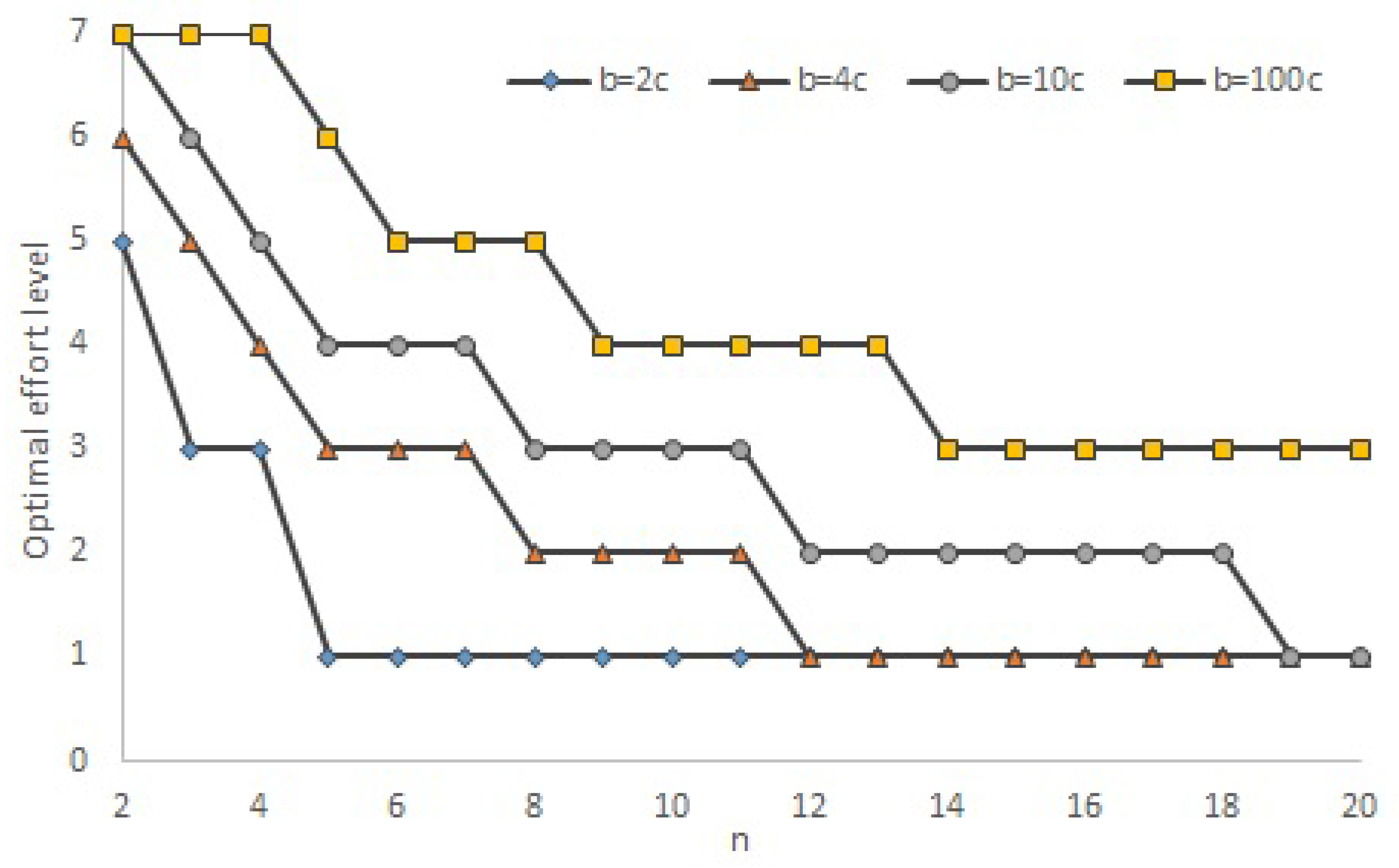
Figure 1 sketches out how the optimal effort level changes as the benefits from coordination are increased, keeping
q the same.
5 You can see that the benefits from coordination have to increase considerably for it to be optimal to choose high effort once
n is 8 or above. So, we obtain a relatively pessimistic picture of the chances of obtaining high efficiency in large groups. On the other hand
Figure 1 suggests that high effort levels may be sustainable if the benefits are sufficiently large. So, there is some positive news.
To put
Figure 1 and the preceding discussion in context, it is important to recognize that we have surprisingly little understanding of what determines long run efficiency in the minimum effort game. We know that, if
, effort levels can be sustained at a high level when
but fall for larger
n (Van Huyck, Battalio and Beil 1990 [
6], Camerer 2003 [
8], Engelmann and Normann 2010 [
9]). Beyond this, evidence is relatively scant. This is primarily because the literature has focused on institutions like leadership, communication and networks that may increase efficiency (Brandts, Cooper and Weber 2014 [
21], Croson et al. 2015 [
22], Riedl, Rohde and Stroble 2015 [
23], Sahin, Eckel and Komai 2015 [
24]). The effect of changes in the benefits and costs of effort are less well known. Theorem 2, in providing a link between optimal effort and the strategic parameters of the game, may provide a novel angle on this issue. In particular,
is easy to calculate, given
q, and so any correlation between this and efficiency would be of interest, however noisy that correlation may be.
In deriving
Figure 1 we kept the initial distribution of effort levels,
q, constant. However, we know that
q will likely vary across different domains. Engelmann and Normann (2010) [
9], for instance, observe a very different distribution of effort levels in the first period with a Danish population. There are other potential variances of framing or environment that could also influence mood and willingness to cooperate such as synchrony or music (Wiltermuth and Heath 2009 [
25], Kniffin et al. 2017 [
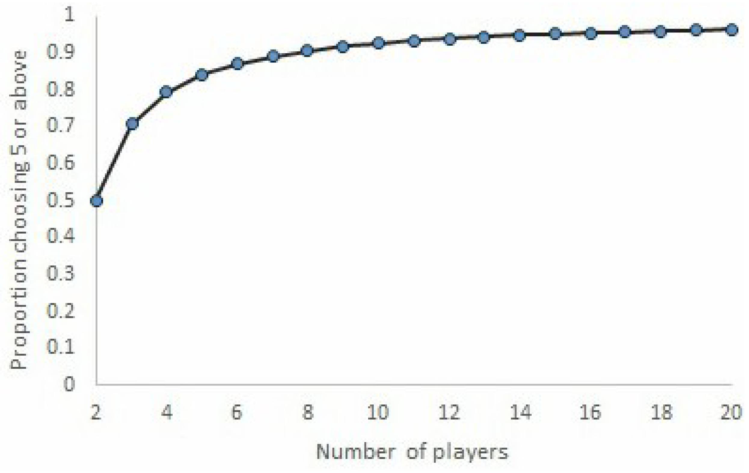
26]). Future work can also, therefore, explore things that may influence initial effort levels. In particular, ‘nudges’ which change first period behavior could be effective in a way that increasing the cost benefit ratio is not. Theorem 2 provides a way to make this comparison more concrete. To illustrate,
Figure 2 plots, as a function of the number of players, the proportion of players (in the population) that must choose 5 or above in order that
. The jump from
to 3 and 4 can help explain why high effort is easier to sustain in small groups. However, interestingly, we see here that an intervention which works for a group of, say, 6 players may well work for larger groups. This provides a more optimistic prediction.


