Abstract
We investigate the role of framing, inequity in initial endowments and history in shaping behavior in a corrupt transaction by extending the one-shot bribery game introduced by Cameron et al. (2009) to a repeated game setting. We find that the use of loaded language significantly reduces the incidence of bribery and increases the level of punishment. Punishment of bribery leads to reduced bribery in future. The evidence suggests that this game captures essential features of a corrupt transaction, over and above any sentiments of inequity aversion or negative reciprocity However, showing subjects the history of past play has little effect on the level of corruption.
JEL Classification:
C91; D73; O17; K42
1. Introduction
We investigate the role of framing, inequity in initial endowments and history in shaping behavior in a corrupt transaction by extending the one-shot bribery game introduced by Cameron et al. (2009) [1] to a repeated game setting. In doing so, we extend the results reported in Cameron et al. (2009) and also address some unresolved questions. Cameron et al. (2009) is an ambitious cross-cultural study, based on experiments involving a corruption game, run in Melbourne, Delhi, Jakarta, and Singapore. Three participants play a one-shot sequential-move game. At the beginning of the experiment each participant is given an initial endowment and assigned to one of three roles: a firm, an official or a citizen. The firm moves first and decides whether or not to offer a bribe to the official. If the firm does not offer a bribe, the game ends. If the firm offers a bribe, she will have to decide on the amount of the bribe. Following this, the official will choose whether to accept or reject the bribe. If the official rejects the bribe, the game ends. If the official accepts the bribe, both the firm and the official’s payoffs increase, vis-à-vis their initial endowments, but this reduces the payoff to the citizen. Then the citizen gets to choose whether or not to punish the act of bribery. If the citizen chooses punishment, this further reduces the citizen’s payoff but reduces the payoff to the firm and the official by a larger magnitude.
Besides looking at cultural differences in behavior in this bribery game, Cameron et al. also explore whether a more effective punishment system deters bribery and whether the cost of bribery, in terms of the negative externality imposed on the citizen, is a factor. They report interpretable differences in behavior across the different subject pools, some of which may be explained by appealing to institutional changes in the relevant societies. They find that more effective punishment, in terms of the punishment amount, can deter corruption, while the magnitude of the negative externality does not have a large impact 1.
In this paper, we will focus only on the “welfare reducing” bribe from Cameron et al. (2009). This is where the total gain from bribery to the firm and the official is less than the payoff loss to the citizen. Specifically, the payoff to the firm and the official is increased by three times the amount of the bribe, while the payoff to the citizen is reduced by seven times the amount of the bribe. Punishment of bribery is costly to all three agents. It reduces the citizen’s payoff by the punishment amount, and reduces the payoffs to the firm and the official by three times the punishment amount. The subgame perfect equilibrium in a one-shot game suggests that a profit maximizing citizen will never punish because punishment is costly to her. Anticipating this, the bribe will always be accepted by the official, and the firm will always offer the largest possible bribe.
In this study, we focus on some unresolved questions, which are primarily, though not entirely, methodological. First, we look at decision making in a repeated play game with random re-matching whereas Cameron et al. look at one-shot plays of the game. While Cameron et al. do use loaded language, which should contribute to removing any possible “cognitive” demand effects (Zizzo, 2010 [4]) nevertheless, one-shot games do not allow for learning or gathering experience about the task at hand. Ours is certainly not the first study to undertake a repeated game analysis of corrupt transactions. Abbink et al. (2002) [5] started off this line of inquiry, which includes other studies such as Azfar and Nelson (2007), [6], Barr et al. (2009) [7] and Jacquemet (2012) [8]. However, there are good reasons for extending the Cameron et al. study to a repeated game setting. The one-shot game in Cameron et al. does not allow them to say much about the impact of punishment in future plays of the game. In order to understand whether punishment can be an effective deterrent to bribery, it is important to have repeated play so that we can see whether a firm, who was punished in one round for bribery, responds by not bribing or bribing less in the next round. Repeated interactions among subjects, with random re-matching from one round to the next, which preserves the one-shot character of the game, allows subjects to get a better understanding of the game. Over time behavior converges to a steady state that is a better representation of true preferences 2.
Second, to what extent does this game capture corrupt behavior? Are there any framing effects? Cameron et al. (2009) are not able to comment on this given that they rely exclusively on loaded language rather than neutral language. Abbink and Hennig-Schmidt (2006) [12] explore whether loaded language, as opposed to neutral language, makes a difference in the context of a bribery game. They report that behavior does not change with a change in the framing of the game. Barr and Serra (2009) [13], on the other hand, find that corruption is lower with loaded language. Cooper and Kagel (2003) [14] also examine this issue, albeit in the context of signalling games. Cooper and Kagel argue that using loaded language makes the underlying strategic imperatives of the game more salient for the players and thereby engage cognitive processes that enable subjects to better understand and address the task at hand.
One major point of departure between the games studied by Abbink and Hennig-Schmidt (2006) [7] and that studied by Cameron et al. (2009) [1] is that the latter allows for an explicit punishment option by a citizen, while the former only allows for a probabilistic punishment of both the firm and the official. By explicitly invoking the notion of a citizen who is harmed by the corrupt acts of the firm and the official and by giving that citizen the power to punish said corruption, Cameron et al. bring underlying issues of ethical behavior and virtuous social norms to the fore-front. Therefore, it is an interesting question to ask whether framing makes a difference in the presence of such “altruistic punishment” (Fehr and Gächter, 2000, 2002, [15,16]) by citizens.
Furthermore, given Cameron et al.’s reliance on loaded language such as “punishment”, they are not able to comment on the real motivation behind punishment. Do citizens punish because they wish to censor corruption on the part of the firm and the official? Or do they punish merely out of negative reciprocity (retribution) given that bribe giving and accepting on the part of the firm and the official increases their payoffs at the expense of the citizen? If it is merely retribution, then we expect to see no dramatic differences with a move from loaded to neutral language. However, if citizens are punishing to discourage corruption, over and above any sentiments of negative reciprocity, then we expect punishment rates to be much higher with loaded language as compared to neutral language.
Third, we explore whether greater inequity in the initial endowment of the players leads to greater corruption? A number of papers have explored this issue prior to us, except the motivation behind these papers is different from ours. Some of these are field studies that focus on the level of compensation for public officials; i.e., they ask whether raising public officials’ wages vis-à-vis a reference wage, such as private sector wages, can be an effective policy instrument in reducing corruption. See for instance di Tella and Schargrodsky (2003) [17], Rauch and Evans (2000) [18], Treisman (2000) [19] and Van Rijckeghem and Weder (2001) [20]. Svensson (2005) [21] provides a survey of this line of work. The evidence is not clear cut. Rauch and Evans (2000) [13] and Treisman (2000) [15] find no correlation while the other two find weak evidence in favour of the hypothesis that raising wages of public officials leads to reduced corruption. Van Veldhuizen (2013) [22] undertakes an experimental study and shows that higher wages lead to significantly lower corruption on the part of officials. However, the result does depend on the frequency of monitoring of the official’s action. Armantier and Boly (2013) [23] is an ambitious study that undertakes both lab and field experiments in Montreal and Ouagadougou (Burkina Faso). They report that raising wages of those marking an exam reduces the propensity to accept a bribe designed to lure the marker into finding fewer mistakes and thereby afford the briber a higher mark. Finally, Jiang et al. (2015) [24] carry out an experimental bribery game in which the potential bribe recipient earned a little bit less than what the potential briber was expected to earn. This payoff inequity served as a justification to offer a bribe.
We approach inequity differently: in terms of the firm’s payoffs with respect to the citizen’s payoffs. Our question is: does inequity between the bribe initiator and the ultimate victim of the bribe play a role in the decision to offer a bribe? In Cameron et al. the authors use a conversion rate from experimental dollars to actual money. If the firm does not offer a bribe, then the game ends with each player receiving the initial endowment. However, these endowments are such that, in the absence of bribery, the citizen is better off than the firm. Given that, the firm has an incentive to offer a bribe, not necessarily because it wishes to engage in corruption but because if it does so and the official accepts then the payoff disparity between the firm and the citizen improves in favour of the former. This implies that an inequity averse firm may be offering a bribe in order to reduce the initial payoff inequity between the firm and the citizen. We will explore this issue below by looking at two different conversion rates, one of which is more inequitable for the firm than the other and see how that impacts firm behavior.
Finally, we ask: How does the history of past corruption and punishment affect current behavior? Schotter and Sopher (2003) [25] argue that in life, when we are confronted with a particular problem or game, we do not operate within a vacuum; but rather we may have access to past history, in the sense of being able to see how other players, who confronted the same problem prior to us, behaved. Access to such history and any advice left by our progenitors can prove useful in developing and sustaining particular social norms. There is now a large literature that explores the role of history and advice in influencing behavior in subsequent generations. Besides, Schotter and Sopher (2003), this literature includes Chaudhuri, Schotter and Sopher (2006, 2009) [26,27], Chaudhuri, Graziano and Maitra (2006) [28] and Schotter and Sopher (2006, 2007), [29,30]. Schotter (2003) [31] provides a partial overview of this line of work. The idea here is similar to that expressed by Fehr and Gächter (2000, 2002), [15,16]; would the presence of altruistic punishers, and information about their existence, make a difference to those engaging in corrupt acts? Or given the random re-matching, would altruistic punishers forego the option to punish? Anticipating this, would firms and officials engage in corruption with impunity?
Banerjee (2016) [32] conducts an experimental study, where he incorporates the notion of prior history by having subjects take part in a bribery game followed by a trust game. He shows that prior experience with a corrupt transaction has a negative spill-over effect in that it leads to lower levels of trust subsequently. There is also a tax compliance literature which shows that providing information regarding past compliance or non-compliance has an impact on current behavior. See, for instance, Trivedi, Shehata and Lynn (2003) [33] or Cadsby, Maynes and Trivedi (2006) [34]. One distinction between Banerjee (2016) [32] and our study or those of Trivedi et al. (2003) [33] or Cadsby et al. (2006) [34] is that, in Banerjee (2016) [32], the nature of the interaction is more “particularized”, in the sense that subjects are interacting within the same session, albeit not with the same partners. So, when playing the trust game, these players are drawing on the history of past interactions in a bribery game with players in the same session. In the other studies including ours, the history information is more “generalized” and refers to decisions taken by subjects in prior sessions, not those in the current one.
We show that the use of loaded language leads to significantly lower levels of bribe giving and acceptance and significantly higher punishment rates. We show, with some caveats, that the incidence of bribery does not increase with an increase in the initial inequity between the firm and the citizen. Therefore, the act of bribery does not seem to be connected to attempts to reduce inequality in initial endowments between the firm and the citizen. These facts, taken together, allow us to claim that the corruption game introduced in Cameron et al. does capture attitudes towards corruption above and beyond sentiments of inequity aversion. Finally, we show that history of past plays does not have much influence on current decisions.
There is now a large literature relying on decision making experiments to study corrupt behavior. We have discussed some related studies above. We will refrain from undertaking a more elaborate review of the related literature. We refer the interested reader to Abbink (2006) [35] as well as the excellent collection of articles in Serra and Wantchekon (2012) [36]; particularly Banuri and Eckel (2012) [37], which provides a comprehensive overview of cultural differences in corruption as well as Chaudhuri (2012) [38], which reviews the literature on gender differences in corrupt behavior. We proceed as follows: Section 2 describes the experimental design, procedures and research questions. Section 3 presents our results while Section 4 concludes.
2. Experimental Methodology
2.1. Experimental Design and Procedures
The game used in this paper is based on the three-person, sequential-move corruption game used by Cameron et al. (2009). Figure 1 summarizes the extensive-form of the game using loaded language with three subjects—Firm, Official and Citizen. Each subject plays only one role for the entire game. We use the repeated-play approach where subjects play this game for ten rounds but they are randomly re-matched at the end of each round so that the same three subjects will not interact with one another for two consecutive rounds. Interactions are anonymous with players being unaware of who the others are in their particular firm-official-citizen triplet. In the case of neutral language, the terms firm, official and citizen are replaced with Player A, Player B and Player C respectively. Emotive words like bribe and punishment are also replaced with neutral terms. Figure 2 shows what the game looks like using neutral language. Appendices A and B provide the instructions for the sessions run with loaded language and neutral language respectively. While the one-shot approach is a logical starting point, the repeated-play approach allows a better understanding of the strategies adopted by participants, and the type of learning that takes place. The payoff of each player is denoted in experimental dollars which are converted to New Zealand dollars at the end of the experiment.

Figure 1.
Structure of the experiment with loaded language.

Figure 2.
Structure of the experiment with neutral language.
At the beginning of each round the firm is endowed with 60 experimental dollars, the official is endowed with 30 experimental dollars, and the citizen is endowed with 80 experimental dollars. The firm moves first and decides whether or not she wants to offer the official a bribe. If the firm decides not to offer a bribe, then the experiment ends and the subjects receive their initial endowments. If the firm decides to offer a bribe, then she has to choose what amount she wants to transfer in the range between 4 and 8, that is, B [4,8]. It costs the firm two experimental dollars to offer a bribe regardless of whether it is accepted or not. Once the firm has decided on the amount to offer to the official, the latter decides whether she accepts this amount or not. If the official decides not to accept the bribe, then the experiment ends with no change in the payoffs to the official or the citizen, while the firm loses 2 experimental dollars from offering the bribe. If the official accepts the bribe, then the payoffs of the firm and the official increase by three times the bribe amount (3B) while the payoff of the citizen decreases by seven times the bribe amount (7B).
The citizen has two choices: to do nothing and accept the resulting payoffs: 58 + 3B for the firm, 30 + 3B for the official and 80 − 7B for the citizen. Or if she wishes, the citizen can forego some more money in order to reduce the payoff to the firm and the official. If the citizen decides to punish, then she has to choose a whole number for that punishment (P) in the range between 2 and 12, that is, P [2,12]. Forgoing money is costly to the citizen; it reduces her payoff by P experimental dollars. However this amount will be multiplied by 3 and the payoffs of the firm and the official will be reduced by this tripled amount. Hence the net payoff of the firm is 58 + 3B − 3P, of the official is 30 + 3B − 3P and of the citizen is 80 − 7B − P.
The subgame perfect equilibrium of the one-shot corruption game is for the firm to offer the maximum bribe, for the official to accept the bribe, and for the citizen to refuse the opportunity to punish. Profit maximizing citizens will not punish, as it is costly. Knowing this the official will accept a bribe, and the firm, in turn, offers the largest possible bribe. Despite this prediction, Alatas et al. (2009a, 2009b) as well as Cameron et al. (2009) find that citizens do punish corruption, not all officials accept bribes, and not all firms offer a bribe. Cameron et al. (2009) report, for instance, that in their Melbourne experiments, 88% of the firms offer a bribe, 89% of the officials accept a bribe when offered and 42% of the citizens punish when the bribe has been offered and accepted.
The experiments are conducted at the University of Auckland in Auckland. The subjects are mostly under-graduate students in business and economics, with no prior experience of the game. There are a total of 210 participants. Each experimental session lasted approximately one hour. At the beginning of each session, each subject is given a copy of the game’s instructions (see Appendices A and B). An experimenter then reads these instructions, with examples, out loud to the subjects. Subjects are then given 10–15 min to read the instructions by themselves, and are offered the opportunity to ask clarifying questions. Then they are provided with instructions regarding how to log in to the computer. The entire experiment is carried out via computers with each subject sitting in a privacy cubicle with partitions on three sides. This prevents subjects from looking at each other’s screens. They are also cautioned against talking, exclaiming or gesticulating in any form during the experiment. Each subject received a NZ $4 show up fee in addition to the earnings from the game. The average total earning was NZ $16, which is approximately equivalent to US $12.30.
2.2. Treatments and Research Questions
We conduct four treatments. In Treatment 1, we maintain parity with the design utilized by Cameron et al. (2009). This is the design that is explained above in Section 2.1, except that subjects in our study play the one-shot game repeatedly for ten rounds with random re-matching between rounds. As in Cameron et al. we use loaded terms like “firm”, “official”, “citizen”, “bribe” and “punishment”. We also use the same conversion rate between experimental earnings and actual dollars. We will refer to this treatment as the “Loaded inequitable” treatment henceforth. This is because, given the conversion rate, this treatment leads to relatively larger disparity in the initial endowments of the firm and the citizen. We will explain this in more detail below when we explain the implementation of the equitable treatment. The roles of firm, official and citizen remain unchanged for the entire session except the triplets are randomly re-matched at the end of each round. At the end of the session, earnings in experimental dollars are converted into cash using the following exchange rate: 60 experimental dollars = NZ $1 for the firm; 40 experimental dollars = NZ $1 for the official and 30 experimental dollars = NZ $1 for the citizen 3. Appendix A contains the instructions for the loaded language treatment. There are 51 subjects (17 triplets) in this treatment generating 170 plays of the game. This serves as our control treatment.
Treatment 2 differs from the Loaded inequitable treatment in that here we use neutral language. Terms such as “firm”, “official” and “citizen” are replaced with “Player A”, “Player B” and “Player C” respectively. The term “offering money transfer” is used instead of “bribe” and “give up more money to reduce the payoff to A and B” replaces the word “punishment” (see Appendix B). There are 60 subjects (20 A-B-C triplets) in this treatment, interacting over ten rounds, generating 200 plays of the game in total. Henceforth, we will refer to this as the “Neutral inequitable” treatment. To what extent does this game capture corrupt behavior? When the citizen chooses to punish the firm and the official, is this merely negative reciprocity (retribution) or does behavior change dramatically when we explicitly introduce terms like “bribe” and “punishment”? In order to answer these questions we compare the bribery and the punishment rates in the Loaded inequitable treatment and the Neutral inequitable treatment.
Treatment 3 is similar to the Loaded inequitable treatment except here the experimental dollars are converted to New Zealand dollars using the same exchange rate of 40 experimental dollars = NZ$1 for all three roles: firm, official and citizen. We will henceforth refer to this as the “Loaded equitable” treatment. This treatment is conducted with 42 subjects, i.e., 14 A-B-C triplets, which generates 140 observations. The Loaded equitable treatment allows us to analyse the underlying causes of bribery in this game. The decision by firms to offer a bribe might have nothing to do with corruption, but rather serve as a means of reducing payoff inequity between the firm and the citizen. In order to analyze the impact of the relative payoff differences between firms and citizens we compare the Loaded equitable treatment to the Loaded inequitable treatment.
For example, in the Loaded inequitable treatment, the initial endowments are: 60 experimental dollars for the firm, 30 for the official and 80 for the citizen. Using the conversion rate used in this treatment (60:1 for the firm; 40:1 for the official and 30:1 for the citizen), this implies the following payoffs in actual dollars: firm gets NZ $1, official gets NZ $0.75 and citizen gets NZ $2.7. Here, in the absence of bribery, the citizen earns 2.7 times what the firm earns. However, in the Loaded equitable treatment, which uses the same conversion rate (40:1) for all three: the firm gets NZ $1.5, the official gets NZ $0.75 and the citizen gets NZ $2. Here, the disparity in the initial endowment is much smaller with the citizen earning 1.3 times the payoff to the firm. Hence, there is a larger payoff difference between the firm and the citizen in the Loaded inequitable treatment than in the Loaded equitable treatment. If initial payoff inequity is the main cause of bribery, then we expect to see more bribes being offered in the Loaded inequitable treatment when compared to the Loaded equitable treatment.
Treatment 4 differs from the Loaded inequitable treatment in that, before subjects make their decisions for round 1, they are shown the following message on the projector. Subjects are told that this information comes from the Loaded inequitable treatment run previously.
Firms offered a bribe in 107 out of 170 cases (63%) and the average bribe offered was 6.73 experimental dollars.The bribe was accepted by the official in 82 cases out of 107 (77%).Out of the 82 cases where the firm offered a bribe and the official accepted, the citizen decided to punish in 59 cases (72%) at an average punishment amount of 8.76 experimental dollars.
The experimenter also reads this message out loud. This treatment is conducted with 57 subjects (19 triplets) generating 190 plays of the game. This treatment will be referred to as the “Loaded inequitable plus history” treatment henceforth. We look at the effect of history on corrupt behavior by comparing the results from the Loaded inequitable treatment to those from the Loaded inequitable plus history treatment. We want to see whether showing subjects the results from previous sessions, demonstrating the presence of punishers, increases or decreases the bribery rate. Table 1 provides a summary overview of the different treatments and the number of observations in each.

Table 1.
Summary of experimental design.
2.3. Hypotheses
On the basis of the discussion in Section 2.2 above, we formulate the following hypotheses.
Hypothesis 1:
Using loaded language will lead to lower corruption; rates of bribe giving and bribe acceptance will be lower and punishment rates will be higher in the Loaded inequitable treatment compared to the Neutral inequitable treatment.
Hypothesis 2:
The bribe rate will be higher when there is greater inequity in the payoff to the firm vis-à-vis the citizen; i.e., we expect more bribes in the Loaded inequitable treatment as opposed to the Loaded equitable treatment.
Hypothesis 3:
Availability of past history will lead to lower corruption, implying lower rates of bribe giving and accepting and higher rates of punishment in the Loaded inequitable plus history treatment compared to the Loaded inequitable treatment.
3. Results
3.1. Overview
In Table 2, we show the rates of bribe giving, bribe acceptance and punishment in Round 1 and aggregated over ten rounds of play. In order to provide some perspective, we also present the corresponding data from one-shot play in Cameron et al. (2009, Table 2, p. 847) [1]. In Round 1, 59% of the firms in our study offered a bribe and the bribe was accepted in 60% of the cases; conditional on the bribe being offered and accepted, 67% of the affected citizens chose to respond with punishment. Averaged over ten rounds, the bribe giving rate is 63%, the bribe acceptance rate is 77% while the punishment rate is 72%. These numbers suggest that the rate of bribe acceptance increased over time (60% in Round 1, 77% on average across ten rounds), while the rates of bribe giving and punishment remained roughly stable over time. We will explore the dynamics of behavior in greater detail in Section 3.3 and Section 3.4 below.
Table 2.
Summary of behavior.
Given the difference in subject pools, direct comparisons are not meaningful. However, it is worth noting that both the rates of bribe giving and bribe acceptance are lower (both in Round 1, as well as, averaged over ten rounds of play), in Auckland compared to the other four locations in Cameron et al. The punishment rate is higher in Auckland, both in Round 1 and averaged over all rounds. It is interesting to note that there is less bribery and greater punishment in Auckland compared to Melbourne, even though, ex ante, one would expect that the nature of the subject pool or the prevailing social norms governing behavior are not all that different in these two locations. However, New Zealand typically ranks well ahead of Australia in the Corruptions Perceptions Index 4. So this could be due to either differences in the subject pool or the fact that subjects know they will be playing repeatedly over ten rounds, or both.
3.2. Analysis of the Role of Framing, History and Inequity Aversion
We begin our analysis by providing a broad brush picture of average behavior across our four treatments and how this lines up with our ex ante hypotheses. Figure 3A–C show what happens to respectively, the bribe rate, acceptance rate and punishment rate over the ten rounds of play. The vertical axis shows the average proportion at which a particular action was taken. So a bribe rate of 0.6 means that on average 60% of the firms offered a bribe in a given round. An acceptance rate of 0.6 means that when a bribe was offered, 60% of the officials in that round chose to accept. Finally, a punishment rate of 0.6 means that when a bribe was both offered and accepted, on average 6 out of 10 citizens chose to punish the firm and the official when given the choice.


Figure 3.
(A) Evolution of the bribe rate over ten rounds; (B) Evolution of the acceptance rate over ten rounds; (C) Evolution of the punishment rate over ten rounds.
Looking at these figures, one thing that stands out is the difference between loaded and neutral language in terms of the bribe and punishment rates. The bribe rate in the Neutral inequitable treatment is equal or close to 1 for all ten rounds; this rate is also visibly higher than that in the Loaded inequitable treatment for all ten rounds. See Figure 3A. The differences between the punishment rates in these two treatments are also obvious, though not as pronounced as that between the bribe rates. (Figure 3C). The punishment rate in the Loaded inequitable treatment is higher than that in the Neutral inequitable for 6 out of 10 rounds; it is also never less than the punishment rate in the Neutral inequitable treatment.
In Table 3, we report results from non-parametric Wilcoxon ranksum tests of equality in distribution between treatments. Given that decisions across the rounds are not independent, we take ten round averages for each individual playing as firm, official or citizen and treat that average as the unit of observation. This gives us 17 observations in each of the three categories in the Loaded inequitable treatment, 20 in the Neutral inequitable treatment, 14 in the Loaded equitable treatment and 19 in the Loaded inequitable plus history treatment 6.
Table 3.
Results of Wilcoxon ranksum tests for bribe, acceptance and punishment rates; average over ten rounds by individual.
Panel 1 of Table 3 addresses the first of our three hypotheses; the extent to which this game captures corrupt behavior by comparing outcomes in the Loaded inequitable treatment with that in the Neutral inequitable treatment. The differences are dramatic. Subjects show higher tolerance for corruption in the Neutral inequitable treatment when compared to the Loaded inequitable treatment. Use of neutral language results in more bribes on average (98% in the Neutral inequitable treatment compared to 63% in the Loaded inequitable treatment) and higher acceptance rates (90% in the former compared to 78% in the latter; though this latter difference is significant only at 10%). Neutral language also results in significantly lower rates of punishment, compared to loaded language, with 56% of citizen choosing to punish in the former compared to 72% in the latter. While the difference between the punishment rates in the two treatments are not significant at conventional levels, punishments amounts are significantly different. Citizens in the Loaded inequitable treatment punished by an average of 8.5 experimental dollars, while those in the Neutral inequitable treatment did so by only 6.7 dollars. This difference is significant at 8%. This is very much in line with our first hypothesis. Bribery is lower with loaded language, while punishment is higher. This suggests that the act of punishment by the citizen in the Loaded inequitable treatment captures disapproval of corruption that goes above and beyond any sentiment of negative reciprocity.
Panel 2 of Table 3 relates to the second hypothesis and examines inequity in initial endowments. Here we compare behavior in the Loaded equitable and the Loaded inequitable treatments. It does not appear that income inequity lies at the heart of bribery. If that were to be the case, then we would expect higher rates of bribe giving in the Loaded inequitable treatment, where the initial endowments are further apart for the firms and the citizens, compared to the loaded equitable treatment. So to close this payoff gap, we expect to see more firms offering bribes in the Loaded inequitable treatment. However our results do not support this conjecture. We find that firms in the Loaded inequitable treatment bribed less than in the Loaded equitable treatment; 63% in the former and 78% in the latter. However, the differences, whether in terms of bribe rates, acceptance rates or punishments rates, are not significant. Taken together, the evidence here does not suggest that income inequity is a major driving force in the desire to engage in corruption.
We do wish to note some caveats about these inequity results. Clearly, changing the exchange rate of the experimental payoffs did not have much of an impact on participants’ behavior. These results do not necessarily imply that inequity aversion cannot explain behavior in this experiment. It is quite possible that our equity manipulation was not successful; for example, because we (a) did not choose the right payoff changes: or (b) changed equity by changing exchange rates rather than payoffs directly, making the changes less salient and possibly less clear to subjects; or (c) decreased inequity between citizen and firm, but increased inequity between firm and public official 7.
Finally, the provision of history of past plays did not result in lower corruption. See Panel 3 of Table 3. We find more bribes in the Loaded inequitable plus history treatment when compared to the Loaded inequitable treatment. 79% of firms offered a bribe in the Loaded inequitable plus history compared to 63% in the Loaded inequitable treatment. But the difference is not significant; neither are the differences in acceptance or punishment rates. Contrary to our ex ante hypothesis, showing subjects history of what happened in the previous session did not reduce bribery. This refutes the third hypothesis above.
Before turning to more formal regression analysis, we ask: was bribery profitable on average? It turns out that the answer is: it depends on whether bribery was punished or not. If and when citizens responded with punishment, on average, bribery did not pay off. In terms of the decision tree in our game, there are four possible options: (1) no bribe offered; (2) bribe offered but not accepted; (3) bribe offered and accepted but not punished and (4) bribe offered and accepted and punished. There are two feasible ways to answer the question of whether bribery paid off. The first is to compare the outcomes in option (1) with those in options (2), (3) and (4); i.e., comparing all cases when the firm did not offer a bribe versus cases where the firm offered a bribe (regardless of what happened after that). Another way of approaching this would be to compare options (1) and (4); when a bribe is not offered, as opposed to when it is offered and punished. If we take the first approach then bribery is profitable; but not if we take the second approach.
In doing this, we take into account all plays of the game, since there is no easy way of computing averages here. Out of 700 total plays of the game, no bribe was offered in 137 cases, with the bribe being offered in the remaining 537 cases. In the 137 cases where a bribe is not offered, the firm gets the default payment of 60 tokens. In the remaining cases the average earning is 62.4 tokens; this difference is significant on a t-test (t = 2.21; p = 0.03). However, in all those cases where bribery was punished, firms made less; i.e., if we compare options (1) and (4). As noted above, there are 137 cases where the firm did not offer a bribe. There are 290 cases where the bribe is offered, accepted and punished. When that happened, on average firms earned 55.7 tokens which is significantly less than the 60 tokens earned when not offering a bribe; (t = 4.5; p < 0.01) 8.
3.3. Bribe and Acceptance Behavior
Given that the observations across the ten rounds of play are not independent, in Section 3.3 and Section 3.4 we examine behavior more rigorously using regression analysis. The regression output we report correspond to non-clustered standard errors 9. Table 4 shows regression results for pooled data from the four different treatments. Columns 1 and 2 present results from a two-part model—a generalisation of the Tobit model—suggested by Cragg (1971) [40] and Cameron and Trivedi (2005) [41]. The first part of the two-part model looks at firm’s decision to offer a bribe or not (Column 1), while the second part looks at the amount of the bribe, given that the firm has decided to bribe (Column 2).
Table 4.
Regression results – effects of framing, history and inequity aversion.
Let be the log-normal of the bribe offered by firm in round and be a bribe indicator for firm in round , where if the firm does not offer a bribe and if the firm offers a bribe. Therefore we have:
is determined by the following equation:
and is determined by the following equation given that :
for and . The random effects are IID and the errors are independent of . The random effects are IID and the errors are independent of . We use random effects rather than fixed effects because each subject has individual-specific effects such as gender, university degree and family background. Here and denote a vector of time invariant effects (like treatment effects), time varying variables (like an individual’s choice in the previous round), and an overall time effect which is common to all players.
For specifications of our model that include lagged values of the dependent variable as one of the independent variables, we correct for dynamic panel data errors by including the first observation of the dependent variable (or initial condition)—either or depending on the model, and either = (Zi1, …, ZiT) or = (Xi1, …, XiT) as independent variables to obtain unbiased coefficient estimates 10. This correction is suggested by Wooldridge (2002, pp. 493–495) [42] for dynamic panel data models of this nature.
Column 1 shows the results of the first part where we regress the bribe rate against the explanatory variables using a random effects Probit model. The dependent variable is either to bribe or not bribe. Independent variables include; (1) dummies for each treatment—Neutral inequitable, Loaded inequitable plus history and Loaded equitable treatments; the Loaded inequitable treatment is used as the reference category, (2) round, (3) interaction terms between each of the three treatment dummies and round, (4) lagged dependent variable (lag bribe), (5) two additional lagged dummies; a dummy for a bribe that is accepted in the previous round (lag bribe with acceptance), and a dummy for punishment after a bribe is accepted in the previous round (lag bribe with punishment).
Wald tests show that the bribe rate is significantly higher in the Neutral inequitable treatment ( = 5.57, p = 0.02) when compared to the Loaded inequitable treatment. This implies that the incidence of bribery goes down when we use loaded language as opposed to neutral language, suggesting that framing the game as a corrupt exchange does make a difference. This provides support for our first hypothesis. The bribe rate for the Loaded equitable treatment is higher than that in the Loaded inequitable treatment but the result is only marginally significant = 3.51, p = 0.06). This provides evidence against the second hypothesis that bribe rate would be higher in the Loaded inequitable treatment. While this may suggest that inequity in initial endowment is not a major driving force behind corruption in this game, nevertheless as noted in Section 3.2 above, this is subject to caveats and it is possible that our inequity manipulation was not appropriate. Finally, the fact that behavior in the history treatment is not different suggests that the third hypothesis is not borne out; showing people history of past plays does not reduce bribe giving 11.
Looking at the incidence of bribery in the immediately preceding round, there are four possibilities: (1) no bribe was offered; (2) bribe was offered but not accepted—“Lag bribe”; (3) bribe offered and accepted but not punished—“Lag bribe with acceptance”; and finally, (4) bribe offered and accepted and punished—“Lag bribe with punishment”. The reference case is (1), i.e., no bribe offered in the previous round, with each dummy being compared to that base case. Looking at the decision to offer a bribe or not in Column 1 of Table 4, this implies that if in the previous round, a bribe was offered but not accepted, the probability of bribing in the current round is lower compared to no bribe in the previous round. The effect of a bribe being not accepted in the previous round is similar to the situation where a bribe was accepted but then punished (coefficient of −0.72 and −0.71 respectively). However, if the bribe was accepted in the previous round but not punished, the probability of bribery increases in the current round. All three effects are highly significant and reinforces the Cameron et al. argument that effective punishment can deter future bribery.
Column 2 shows the results of the second part of the two-part model where we use a random effects maximum likelihood regression on a log-normal of the bribe amount given that the firm chose to offer a bribe 12. Independent variables in the second part are the same as for the first, with the addition of the log-normal of the amount of the bribe offered by subject i in the previous round (lag ln(bribe amount)) 13. The bribe amount offered is not significantly different across the four treatments ( (3) = 1.02, p = 0.80). The estimated coefficients for lag bribe, lag bribe with acceptance, and lag bribe with punishment are not statistically significant which suggests that whether a bribe is accepted or whether a citizen punished bribery in the previous round does not have a significant impact on the bribe amount in the current round. The estimated coefficient for the lag ln(bribe amount) variable is positive and significant, suggesting that a higher (lower) bribe amount in the previous round will lead to a higher (lower) bribe in the current round.
In conclusion, our two-part model shows that firms offer a bribe significantly more often in the Neutral inequitable treatment and marginally more often in the Loaded equitable treatment when compared to the Loaded inequitable treatment. Being punished for bribery in the past reduces bribe giving in the future. However the bribe amounts are not significantly different across the four different treatments. The history of bribery and punishment do not have a significant impact on the rate at which bribes are offered.
Column 3 relates to the officials’ acceptance rate given that a bribe is offered. We use a random effects Probit regression for the officials’ acceptance decision - accept or reject - as the dependent variable. Independent variables include; (1) three treatment dummies with the Loaded inequitable treatment being the reference category; (2) round; (3) interaction terms between treatment dummies and round; (4) bribe amount offered by a firm; (5) interaction terms between the three treatment dummies and the bribe amount offered by a firm; (6) the lagged dependent variable (lag acceptance); and (7) a dummy for punishment after a bribe is accepted in the previous period (lag acceptance with punishment) 14.
Wald tests show that the bribe acceptance rate is significantly lower in the Loaded equitable compared to Loaded inequitable equitable treatment ( (1) = 4.06, p = 0.04). The interaction term between the Loaded inequitable plus history treatment dummy and round is negative suggesting that the availability of past history has some positive impact on reducing corruption over time but the effect seems small, given the marginal significance of the relevant coefficient. The effect of the bribe amount on the acceptance rate is positive for all four treatments, but this effect is only significant in the Neutral inequitable and the Loaded equitable treatments. This suggests that the higher the bribe amount offered, the more likely it is that the officials in these two treatments will accept those bribes.
If we look at lagged acceptance rates, as we did with the bribe rate, the base case is where the bribe is not accepted, which is compared to (1) bribe accepted but not punished—lag acceptance and (2) bribe accepted and punished—lag acceptance with punishment. The estimated coefficient for the lag acceptance with punishment is negative and significant suggesting that if the officials are punished in the previous round, they will be less willing to accept bribes in the current round. Taken together, these results demonstrate that punishment of corruption reduces corruption, both for bribe giving and acceptance. This corroborates the results in Cameron et al. (2009) who also argue that effective punishment can lower corruption.
3.4. Punishment Behavior
In this section, we explore punishment behavior across treatments. Again, we use the two-part model to investigate punishment behavior. Column 4 reports results for the first part regarding whether to punish or not, given that a bribe has been offered and accepted. Column 5 reports the results for the second part, which deals with the actual magnitude of the punishment. Independent variables include; (1) three treatment dummies with the Loaded inequitable treatment being the reference category; (2) round; (3) interaction terms between each treatment dummy and round; (4) bribe amount offered by a firm; and (5) the lagged dependent variable (lag punishment) 15.
Wald tests show that the punishment rate in the Neutral inequitable treatment is lower than the Loaded inequitable treatment ( (1) = 2.88, p = 0.09). The citizens punish more often in the treatment which uses loaded language and frames the game as a corrupt transaction as opposed to the treatment where we use neutral language. The coefficient on round is negative and significant suggesting that the frequency of punishment by the citizen decreases over time in all four treatments. But this coefficient is positive and marginally significant for the interaction term between the Neutral inequitable treatment dummy and round, suggesting that the decline is slower in this treatment but the effect is not large. The estimated coefficient for bribe amount is positive and significant, meaning that the higher the bribe amount offered and accepted, the higher is the likelihood that the citizen punishes.
Column 5 reports the results of a random effects maximum likelihood regression with the log-normal of the punishment amount (given that bribe is offered, accepted, and the citizen decided to punish) as the dependent variable. Independent variables in the second part are the same as in the first except that the lag punishment variable is replaced with the lagged log-normal of the punishment amount (lag ln(punishment amount)) 16. The estimated coefficient for the bribe amount offered by firms is positive and significant suggesting that the higher the bribe amount, the higher the punishment amount. The estimated coefficient for the lag dependent variable is positive and significant which means that the punishment amount is dependent on the citizens’ past punishment behavior. Given the log-log formulation, this suggests that a 10% increase in previous punishment amount would result in an approximately 4% increase in current punishment amount. The more (less) the citizen punished in the last period, the more (less) the citizen punishes in the current period.
To summarize: the use of loaded language does lead to a significant reduction in corruption, in terms of reduced bribe giving and accepting and increased punishment for corruption. Contrary to the second hypothesis, it does not appear that endowment inequity is a major factor behind the decision to offer a bribe. If inequity was a factor, we should have seen a higher bribe rate in the inequitable treatment compared to the equitable treatment. However, as noted before, this result is subject to the caveat that subjects may not have understood the change in exchange rates and therefore our experimental manipulation may not have succeeded. We do not find support for the third hypothesis: that showing people the history of prior plays will reduce corruption and increase punishment. We find some evidence that the availability of past history reduces bribe acceptance, but the effect is small.
The fact that past history did not matter is surprising in light of prior studies cited above. In retrospect, it is possible that the conflicting nature of the information given is one reason why history did not make a difference in our experiment. The information provided shows both the occurrence of bribery as well as punishment and it is possible that neither of these two bits of information stood out for the subjects. Or, it is possible that some picked up on the bribery aspect while others picked up on the punishment aspect with neither prevailing over the other.
4. Concluding Remarks
In this paper, we address some unresolved questions arising from the results reported in Cameron et al. (2009). We show that the use of loaded language, as opposed to neutral language, leads to dramatic reduction in corruption and increase in punishment. We have extended and reinforced the finding that being punished for bribe giving in the past leads to reduced bribery in the future. We have also shown that the decision to offer a bribe is not driven primarily by a desire to address inequities in initial endowments. Collectively, these results suggest that the Cameron et al. corruption game with loaded language captures essential features of a corrupt transaction over and above any sentiments of inequity aversion or negative reciprocity. While these results are in line with our ex ante hypotheses, contrary to our conjecture, we find that showing subjects history of past plays has little effect on corruption via marginally lower bribe acceptance rates but no effect on the bribe or punishment rates. It is possible that the information provided contradictory messages, with some subjects focusing on the fact of bribery while others focused on the punishment.
There is now increasing evidence that suitable framing can lead to sharp differences in behavior. Relevant studies include Cadsby et al. (2006) [34] who look at the issue of framing in tax compliance experiments or Chaudhuri et al. (2016) [43] who explore notions of trust and trustworthiness. Cooper and Kagel (2003, p. 312) [14] comment that economists tend to prefer abstract language in instructions possibly because of “… the belief that it is only the deep, underlying mathematical structure of the problem that matters (or should matter) for behavior … Yet there are important reasons to study behavior in natural settings since there is abundant evidence that subjects’ reasoning processes can be affected in fundamental ways when problems are embedded in meaningful, as opposed to abstract or generic, context.” Samuelson (2005, pp. 94–96) [44], elaborates on this idea by stating: “. . . interpretation of experimental results can then depend importantly on how we imagine participants perceive the game . . . Despite an experimenter’s best efforts to ensure that participants understand what they are dealing with, . . . it is not clear when we can be confident that the participants’ models match the experimenter’s.” Levati, Miettinen and Rai (2011, p. 847) [45] add: “An important component of the requirement that a participant’s model of a situation matches the experimenter’s model is that the participant and the experimenter should attach the same meanings to the elements in the action sets of the agents involved in an interaction.” Taken together, the evidence presented here highlights the importance of suitable framing, via the use of emotive language, for studying corruption and/or other types of unethical behaviour in the lab. In turn, such framing can also potentially play a significant role in trying to address such issues in a policy context.
Acknowledgments
We thank the University of Auckland for providing the funds needed for this study. We thank Alan Rogers, Lata Gangadharan and Maros Servatka for feedback. We thank three anonymous referees of this journal for detailed and thoughtful comments, which have significantly improved the paper’s exposition.
Author Contributions
All authors contributed equally.
Conflicts of Interest
The authors declare no conflicts of interest.
Appendix A: Instructions for the Loaded Inequitable Treatment
Instructions
General
This is an experiment in the economics of decision making. Funding for this research has been provided by the University of Auckland. The instructions are simple. If you follow them carefully, you will earn money that will be paid to you privately in cash at the end of today’s session. This money is in addition to the show-up fee that you get. Please do not talk to each other during the experiment.
In today’s experiment you will be a part of a group of three players. You will be presented with a real-life-like situation, where you will be randomly assigned to the role of the Manager of a Firm, a Government Official, or a Citizen. You will play the game for 10 rounds. Your role will remain unchanged for the entire time. That is you will be a firm, or an official or a citizen for all 10 rounds. You will not know who the other players are in the group in any round. The composition of the group will change from one round to the next. That is, the same three players will not be part of a firm-official-citizen trio for more than one round.
The money that you make in this experiment will be called payoffs. Payoffs in this experiment are denoted in experimental dollars. At the end of this session, these experimental dollars will be converted into cash using the following exchange rate: For the Firm the exchange rate is 60 experimental dollars = NZ $1, for the Official it is 40 experimental dollars = NZ $1 and the Citizen it is 30 experimental dollars = NZ $1.
In this experiment, participants will make decisions in turn. The Firm moves first and decides whether it wants to offer the Official a bribe or not. If the Firm decides not to offer a bribe, then the experiment ends. If the Firm decides to offer a bribe, then the Firm has to choose what amount to offer. Once the Firm has decided on the amount to offer to the Official, the Official gets to decide whether s/he accepts the bribe or not. If the Official decides not to accept the bribe, then the experiment ends. If the Official accepts the bribe, then the Citizen gets the chance to move. The Citizen has two choices: to punish the Firm and the Official for offering and accepting the bribe respectively, or not to punish them. If the Citizen decides not to punish, then the experiment ends. If the Citizen decides to punish, then s/he has to decide on a monetary amount of that punishment.
Detailed Instructions for Firms
In today’s experiment, if you are a Firm, then you have to decide whether to offer the Official a bribe or not using the options on your computer screen. If you decide not to offer a bribe, then the experiment ends and the participants get the following amounts: the Firm gets 60 experimental dollars, the Official gets 30 experimental dollars, and the Citizen gets 80 experimental dollars. If you choose to offer a bribe, then you have to choose how much to offer. You incur a cost of 2 experimental dollars for offering this bribe regardless of whether the Official accepts it or not. You can choose to offer an amount B, where B can be a whole number in between 4 and 8, i.e., B = (4, 5, 6, 7, 8). If you as the Firm decided to offer a bribe, then the experiment continues and the Official gets to make his/her decision. Your payoff will be determined at the end of the game according to the decisions made by all of the players in your group.
Detailed Instructions for Officials
On your screen you will get to see the decision made by the Firm in your group. After observing this, you get to make your decision. If the Firm in your group has offered you a bribe (B), you have to now decide whether to accept the bribe or not. If you decide not to accept the bribe, then the experiment ends with the Firm getting 58, the Official getting 30, and Citizen getting 80 experimental dollars. If you accept the bribe, then conditional on the Citizen’s actions the payoffs can be of two types. If the Citizen decides not to punish, then the following payoffs occur: Firm gets 58 + 3B, Official gets 30 + 3B, and Citizen gets 80 − 7B, where B is the amount of bribe offered by the Firm. If the Citizen decides to punish, then the following payoffs occur: Firm gets 60 − 2 + 3B − 3P, Official gets 30 + 3B − 3P and the Citizen gets 80 − 7B − P, where P is the amount of punishment chosen by the Citizen. The payoffs indicate that the bribe B offered by the firm gets multiplied by 3, if you decide to accept the bribe but this in turn will reduce the citizen’s payoff by 7 times the amount of the bribe.
Detailed Instructions for Citizens
If you are a Citizen in today’s experiment, on your computer screen you will get to see the decisions made by the Firm and the Official in your group. If the Firm and the Official in your group has offered and accepted a bribe respectively, your payoff automatically gets reduced by 7 times the amount of the bribe, B. This is the harm you suffer as a result of the act of bribery. You can punish them if you wish. If you choose to punish, then you can choose a whole number in between 2 and 12, i.e., P = (2, 3, 4, 5, 6, 7, 8, 9, 10, 11, 12) as the amount of the punishment. The monetary amount of punishment that you choose will be multiplied by 3, and the payoffs of the Official and the Firm will be reduced by this tripled amount. Your payoff will be reduced by $P, the amount of punishment you have chosen. The exact payoffs will be: Firm gets 58 + 3B − 3P, Official gets 30 + 3B − 3P, and Citizen gets 80 − 7B − P. If you decide not to punish, then the payoffs will be: Firm gets 58 + 3B, Official gets 30 + 3B, and Citizen gets 80 − 7B.
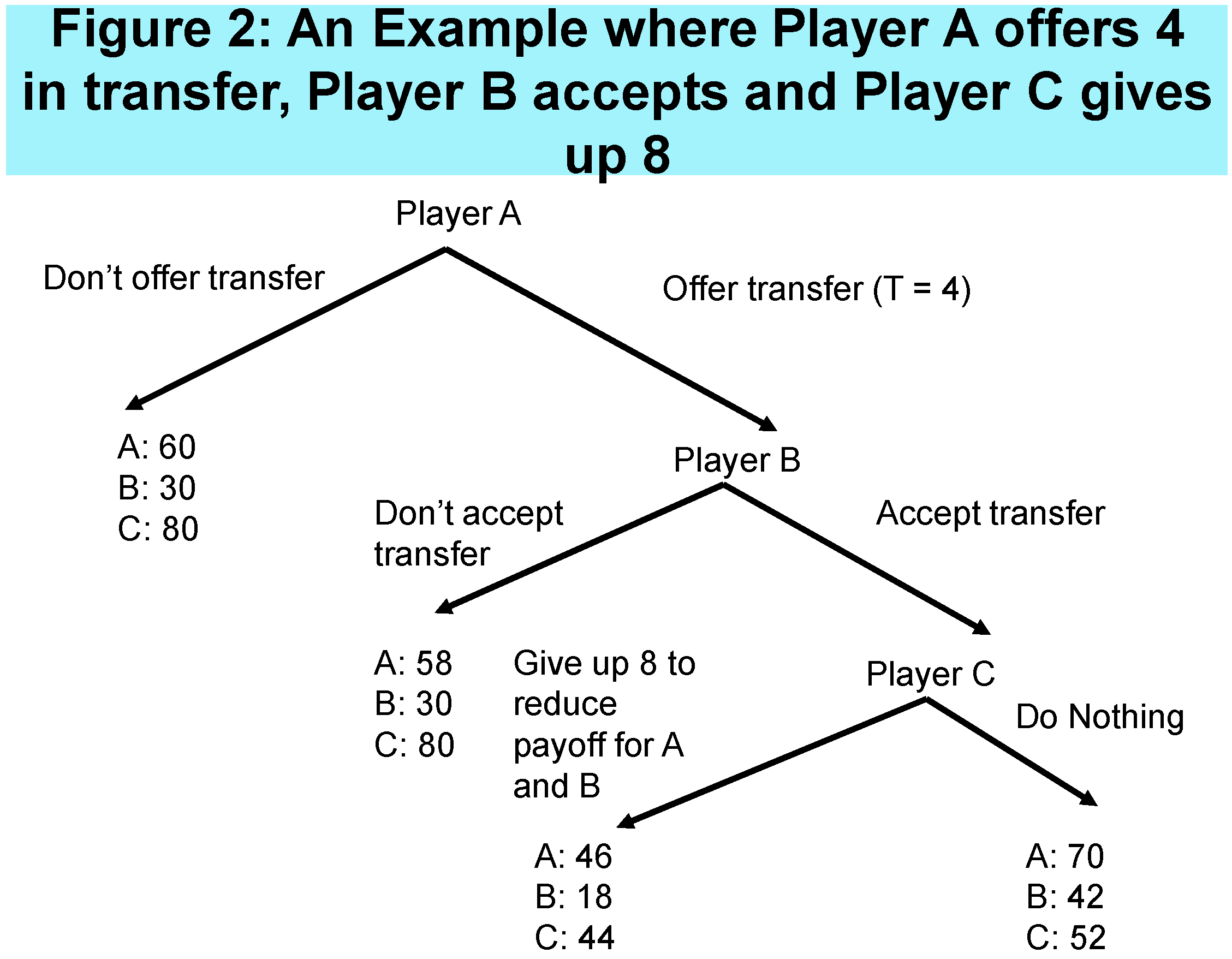
Figure A1 describes the general set-up of this game and the sequence of decisions. Figure A2 describes an example of what would happen and what the payoffs would be if the Firm chooses to offer 4 experimental dollars in bribe, the Official chooses to accept, and the Citizen decides to punish the Firm and Official by 8 experimental dollars. Notice that in this case the payoffs to the Firm and the Official get reduced by 24 experimental dollars while the payoff to the Citizen gets reduced by 8 experimental dollars.

Figure A1.
The structure of the experiment.
Figure A1.
The structure of the experiment.
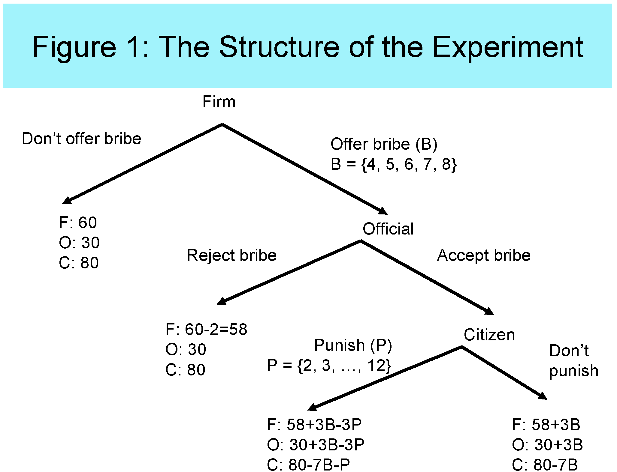
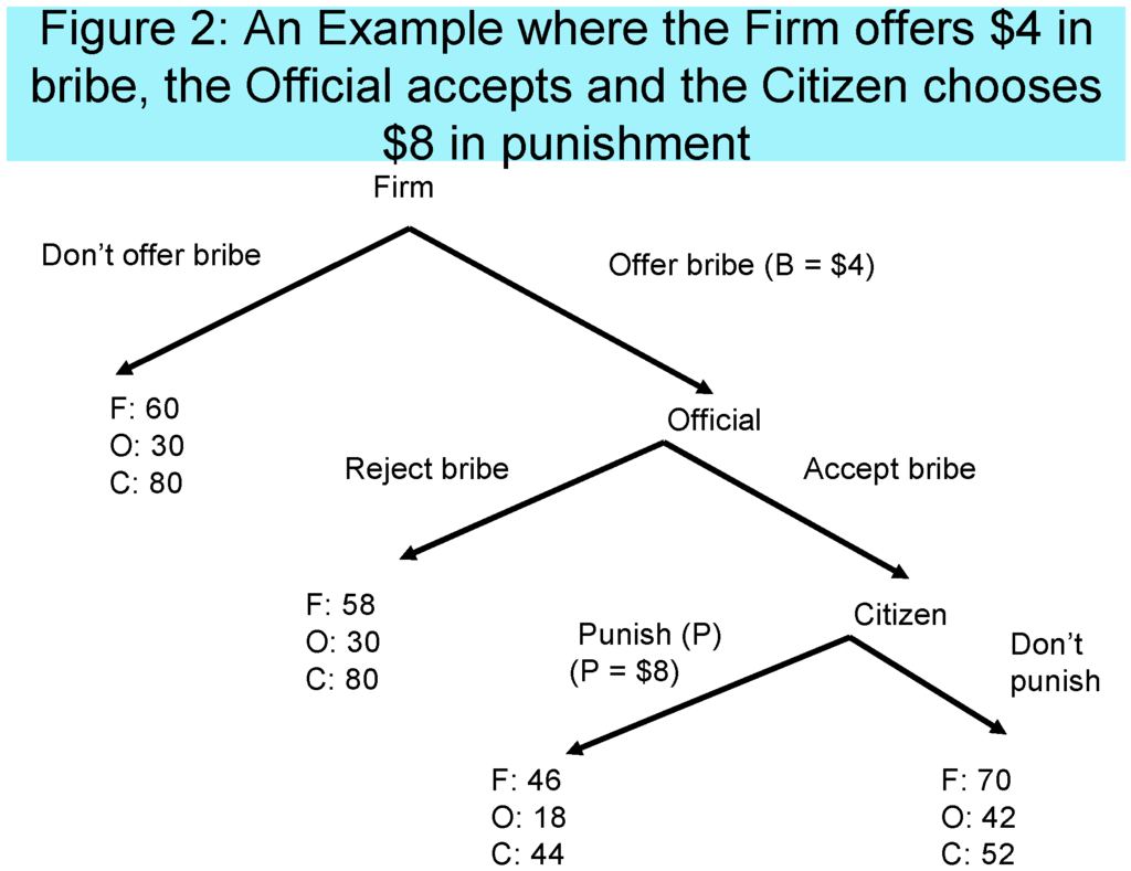
Figure A2.
An illustrative example.
Figure A2.
An illustrative example.
Appendix B: Instructions for the Neutral Inequitable Treatment
Instructions
General
This is an experiment in the economics of decision making. Funding for this research has been provided by The University of Auckland. The instructions are simple. If you follow them carefully, you will earn money that will be paid to you privately in cash at the end of today’s session. Please do not talk to each other during the experiment.
In today’s experiment each of you will be a part of a group of three players. These three players will be selected as player A, player B and player C respectively. Once you have logged on, you will be randomly assigned to your role in the experiment. You will play the game for 10 rounds. Your role will remain unchanged for the entire time. That is you will be player A, player B or player C for all 10 rounds. You will not know who the other players are in the group in any round. The composition of the group will change from one round to the next. That is, the same three players will not be part of a player A-player B-player C trio for more than one round.
The money that you make in this experiment will be called payoffs. Payoffs in this experiment are denoted in experimental dollars. At the end of this session, these experimental dollars will be converted into cash using the following exchange rate: For Player A the exchange rate is 60 experimental dollars = NZ $1, for Player B it is 40 experimental dollars = NZ $1 and for Player C it is 30 experimental dollars = NZ $1.
In this experiment, participants will make decisions in turn. Player A moves first and decides whether s/he wants to offer Player B a monetary transfer (an amount of money) or not. If Player A decides not to offer this amount, then the experiment ends. If Player A decides to offer this amount, then Player A has to choose what amount to offer. Once Player A has decided on the amount to offer to Player B, Player B gets to decide whether s/he accepts this amount or not. If Player B decides not to accept this transfer, then the experiment ends. If Player B accepts the transfer, then the total payoff to both Players A and B will increase but at the expense of the payoff to Player C. This means that if Player A offers the transfer and Player B accepts it, then Player C’s payoff decreases. Player C then has two choices: to do nothing and take the payoff that s/he gets in this case. On the other hand if s/he wishes, Player C can forego some more money in order to reduce the payoff to Players A and B.
Detailed Instructions for Player A
In today’s experiment, if you are Player A, then in each round, you have to decide whether to offer Player B a money transfer or not. If you decide not to offer a transfer, then the experiment ends and the participants get the following amounts: Player A gets 60 experimental dollars, Player B gets 30 experimental dollars, and Player C gets 80 experimental dollars. If you choose to offer a transfer, then you have to choose how much to offer. You incur a cost of 2 experimental dollars for offering this transfer regardless of whether Player B accepts it or not. You can choose to offer an amount (T) which can be a whole number in between 4 and 8, i.e., T = (4, 5, 6, 7, 8). If you, as Player A, decided to offer a transfer, then the experiment continues and Player B gets to make his/her decision. Your payoff will be determined at the end of the game according to the decisions made by all three players in your group.
Detailed Instructions for Player B
On your screen you will get to see the decision made by player A in your group. After observing this, you get to make your decision. If Player A in your group has offered you a transfer (T), you have to now decide whether to accept this transfer or not. If you decide not to accept the transfer, then the experiment ends with Player A getting 58 experimental dollars, Player B getting 30 experimental dollars, and Player C getting 80 experimental dollars. If you accept the transfer, then conditional on Player C’s actions the payoffs can be of two types. If Player C decides to do nothing, then the following payoffs occur: Player A gets 58 + 3T, Player B gets 30 + 3T, and Player C gets 80 − 7T, where T is the amount of transfer offered by Player A. If C decides to give up some of her money in order to reduce the payoff to Player A and Player B. For every experimental dollar that Player C gives up, the payoff to Player A and Player B will be reduced by 3 experimental dollars. So if Player C gives up G experimental dollars then Player A gets 58 + 3T − 3G, Player B gets 30 + 3T − 3G and Player C gets 80 − 7T − G, where G is the amount of money given up by Player C. The payoffs indicate that amount T offered by Player A gets multiplied by 3, if you decide to accept this amount, but this in turn will reduce player C’s payoff by 7 times the amount T offered.
Detailed Instructions for Player C
If you are Player C in today’s experiment, in each round on your computer screen you will get to see the decisions made by Player A and Player B in your group. If Player A and Player B in your group has offered and accepted the transfer respectively, your payoff automatically gets reduced by 7 times the amount of the transfer (T). In response, you can choose to do nothing or if you wish you can reduce the payoff to Players A and B by giving up some of your money. If you do wish to give up some of your money in order to reduce the payoff to Player A and Player B, then you can choose a whole number (G) in between 2 and 12, i.e., G = (2, 3, 4, 5, 6, 7, 8, 9, 10, 11, 12) as the amount. The amount that you give up will be multiplied by 3, and the payoffs of Player A and Player B will be reduced by this tripled amount. Your payoff will be reduced by G experimental dollars, the amount of money you have chosen to give up. The exact payoffs will be: Player A gets 58 + 3T − 3G, Player B gets 30 + 3T − 3G, and Player C gets 80 − 7T − G. If you decide not to give up any money, then the payoffs will be: Player A gets 58 + 3T, Player B gets 30 + 3T, and Player C gets 80 − 7T.
Figure B1 describes the general set-up of this game and the sequence of decisions. Figure B2 describes an example of what would happen and what the payoffs would be if Player A chooses to offer 4 experiment dollars in transfer, Player B chooses to accept, and Player C decides to give up 8 experimental dollars. Notice that in this case the payoffs to Player A and Player B get reduced by 24 experimental dollars while the payoff to Player C gets reduced by 8 experimental dollars.

Figure B1.
The structure of the experiment.
Figure B1.
The structure of the experiment.
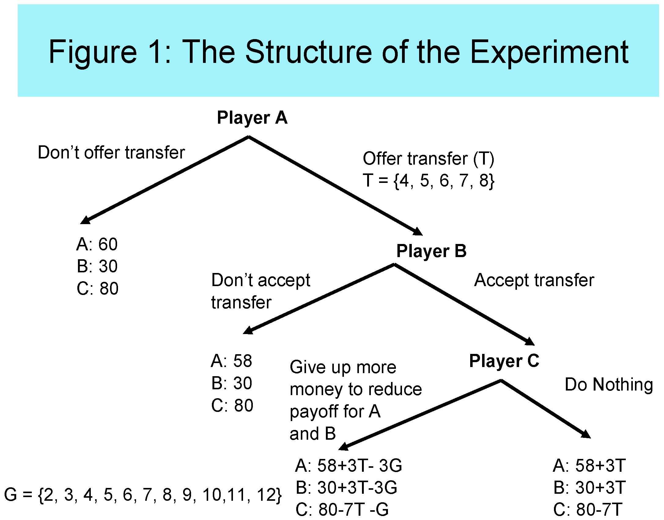

Figure B2.
An illustrative example.
Figure B2.
An illustrative example.
References
- Cameron, L.; Chaudhuri, A.; Erkal, N.; Gangadharan, L. Propensities to engage in and punish corrupt behavior: Experimental evidence from Australia, India, Indonesia and Singapore. J. Public Econ. 2009, 93, 843–851. [Google Scholar] [CrossRef]
- Alatas, V.; Cameron, L.; Chaudhuri, A.; Erkal, N.; Gangadharan, L. Gender and Corruption: Insights from an Experimental Analysis. South. Econ. J. 2009, 75, 663–680. [Google Scholar]
- Alatas, V.; Cameron, L.; Chaudhuri, A.; Erkal, N.; Gangadharan, L. Subject pool effects in a corruption experiment: A comparison of Indonesian public servants and Indonesian students. Exp. Econ. 2009, 12, 113–132. [Google Scholar] [CrossRef]
- Zizzo, J. Experimenter demand effects in economic experiments. Exp. Econ. 2010, 13, 75–98. [Google Scholar] [CrossRef]
- Abbink, K.; Irlenbusch, B.; Renner, E. An experimental bribery game. J. Law Econ. Organ. 2002, 18, 428–454. [Google Scholar] [CrossRef]
- Azfar, O.; Nelson, W. Transparency, Wages, and the Separation of Powers: An Experimental Analysis of Corruption. Public Choice 2007, 130, 471–493. [Google Scholar] [CrossRef]
- Barr, A.; Lindelow, M.; Serneels, P. Corruption in public service delivery: An experimental analysis. J. Econ. Behav. Organ. 2009, 72, 225–239. [Google Scholar] [CrossRef]
- Jacquemet, N. Corruption as Betrayal: Experimental Evidence; Mimeo, Université Paris 1 Panthéon-Sorbonne: Paris, France, 2012. [Google Scholar]
- Andreoni, J.; Croson, R. Partners versus strangers: Random rematching in public goods experiments. In Handbook of Experimental Economics Results; Plott, C., Smith, V., Eds.; Elsevier: Amsterdam, North Holland, The Netherlands, 2008; Chapter 82; pp. 772–776. [Google Scholar]
- Kreps, D.; Milgrom, P.; Roberts, J.; Wilson, R. Rational cooperation in the finitely repeated prisoners’ dilemma. J. Econ. Theory 1982, 27, 245–252. [Google Scholar] [CrossRef]
- Benoit, J-P.; Krishna, V. Finitely Repeated Games. Econometrica 1985, 53, 905–922. [Google Scholar]
- Abbink, K.; Hennig-Schmidt, H. Neutral versus Loaded Instructions in a Bribery Experiment. Exp. Econ. 2006, 9, 103–121. [Google Scholar] [CrossRef]
- Barr, A.; Serra, D. The effects of externalities and framing on bribery in a petty corruption experiment. Exp. Econ. 2009, 12, 488–503. [Google Scholar] [CrossRef]
- Cooper, D.; Kagel, J. The Impact of Meaningful Context on Strategic Play in Signalling Games. J. Econ. Behav. Organ. 2003, 50, 311–337. [Google Scholar] [CrossRef]
- Fehr, E.; Gächter, S. Cooperation and Punishment in Public Goods Experiments. Am. Econ. Rev. 2000, 90, 980–994. [Google Scholar] [CrossRef]
- Fehr, E.; Gächter, S. Altruistic Punishment in Humans. Nature 2002, 415, 137–140. [Google Scholar] [CrossRef] [PubMed]
- Di Tella, R.; Schargrodsky, E. The role of wages and auditing during a crackdown on corruption in the city of Buenos Aires. J. Law Econ. 2003, 46, 269–292. [Google Scholar] [CrossRef]
- Rauch, J.; Evans, P. Bureaucratic structure and bureaucratic performance in less developed countries. J. Public Econ. 2000, 75, 49–71. [Google Scholar] [CrossRef]
- Treisman, D. The causes of corruption: A cross-national study. J. Public Econ. 2000, 76, 399–457. [Google Scholar] [CrossRef]
- Van Rijckeghem, C.; Weder, B. Bureaucratic corruption and the rate of temptation: Do wages in the civil service affect corruption, and by how much? J. Dev. Econ. 2001, 65, 307–331. [Google Scholar] [CrossRef]
- Svensson, J. Eight questions about corruption. J. Econ. Perspect. 2005, 19, 19–42. [Google Scholar] [CrossRef]
- Van Veldhuizen, R. The influence of wages on public officials’ corruptibility: A laboratory investigation. J. Econ. Psychol. 2013, 39, 341–356. [Google Scholar] [CrossRef]
- Armantier, O.; Boly, A. Comparing corruption in the laboratory and in the field in Burkina Faso and Canada. Econ. J. 2013, 123, 1168–1187. [Google Scholar] [CrossRef]
- Jiang, T.; Lindemans, J.W.; Bicchieri, C. Can trust facilitate bribery? Experimental evidence from China, Italy, Japan and the Netherlands. Soc. Cognit. 2015, 33, 483–504. [Google Scholar] [CrossRef]
- Schotter, A.; Sopher, B. Social Learning and Coordination Conventions in Intergenerational Games: An Experimental Study. J. Political Econ. 2003, 111, 498–529. [Google Scholar] [CrossRef]
- Chaudhuri, A.; Schotter, A.; Sopher, B. Learning in Tournaments with Inter-generational Advice. Econ. Bull. 2006, 3, 1–16. [Google Scholar]
- Chaudhuri, A.; Schotter, A.; Sopher, B. Coordination in inter-generational minimum games with private, almost common and common knowledge of advice. Econ. J. 2009, 75, 91–122. [Google Scholar] [CrossRef]
- Chaudhuri, A.; Graziano, S.; Maitra, P. Social Learning and Norms in an Experimental Public Goods Game with Inter-Generational Advice. Rev. Econ. Stud. 2006, 73, 357–380. [Google Scholar] [CrossRef]
- Schotter, A.; Sopher, B. Advice, Trust and Trustworthiness in an Experimental Intergenerational Game. Exp. Econ. 2006, 9, 123–145. [Google Scholar] [CrossRef]
- Schotter, A.; Sopher, B. Advice and Behavior in Intergenerational Ultimatum Games: An Experimental Approach. Games Econ. Behav. 2007, 58, 365–393. [Google Scholar] [CrossRef]
- Schotter, A. Decision making with naïve advice. Am. Econ. Rev. Pap. Proc. 2003, 93, 196–201. [Google Scholar] [CrossRef]
- Banerjee, R. Corruption, Norm Violation and Decay in Social Capital. J. Public Econ. 2016, 137, 14–27. [Google Scholar] [CrossRef]
- Trivedi, V.; Shehata, M.; Lynn, B. Impact of Personal and Situational Factors on Taxpayer Compliance: An Experimental Analysis. J. Bus. Eth. 2003, 47, 175–197. [Google Scholar] [CrossRef]
- Cadsby, C.B.; Maynes, E.; Trivedi, V.U. Tax compliance and obedience to authority at home and in the lab: A new experimental approach. Exp. Econ. 2006, 9, 343–359. [Google Scholar] [CrossRef]
- Abbink, K. Laboratory experiments on corruption. In International Handbook on the Economics of Corruption; Rose-Ackerman, S., Ed.; Edward Elgar Publishers: Cheltenham, UK, 2006; Chapter 14; pp. 418–437. [Google Scholar]
- Serra, D.; Wantchekon, L. (Eds.) Research in Experimental Economics Volume 15: New Advances in Experimental Research on Corruption; Emerald Group Publishing: Bingley, UK, 2012.
- Banuri, S.; Eckel, C. Experiments in culture and corruption: A review. In Research in Experimental Economics Volume 15: New Advances in Experimental Research on Corruption; Serra, D., Wantchekon, L., Eds.; Emerald Group Publishing: Bingley, UK, 2012; Chapter 3; pp. 51–76. [Google Scholar]
- Chaudhuri, A. Gender and corruption: A survey of the experimental evidence. In Research in Experimental Economics Volume 15: New Advances in Experimental Research on Corruption; Serra, D., Wantchekon, L., Eds.; Emerald Group Publishing: Bingley, UK, 2012; Chapter 2; pp. 13–49. [Google Scholar]
- Cameron, C.; Miller, D. A Practitioner’s Guide to Cluster-Robust Inference. J. Hum. Resour. 2015, 50, 317–373. [Google Scholar] [CrossRef]
- Cragg, J.G. Some Statistical Models for Limited Dependent Variables with Application to the Demand for Durable Goods. Econometrica 1971, 39, 829–844. [Google Scholar] [CrossRef]
- Cameron, A.C.; Trivedi, P.K. Microeconometrics Methods and Applications; Cambridge University Press: Cambridge, UK, 2005. [Google Scholar]
- Wooldridge, J. Econometric Analysis of Cross Section and Panel Data; MIT Press: Cambridge, MA, USA, 2002. [Google Scholar]
- Chaudhuri, A.; Paichayontvijit, T.; Li, Y. Context, Common Knowledge, Trust and Reciprocity; Working Paper; Department of Economics, University of Auckland: Auckland, New Zealand, 2016. [Google Scholar]
- Samuelson, L. Economic Theory and Experimental Economics. J. Econ. Lit. 2005, 43, 65–107. [Google Scholar] [CrossRef]
- Levati, M.; Miettinen, T.; Rai, B. Context and interpretation in laboratory experiments: The case of reciprocity. J. Econ. Psychol. 2011, 32, 846–856. [Google Scholar] [CrossRef]
- 1Alatas et al. (2009a) [2] use the same game, undertaken across the four different locations, to look for gender differences in behavior. Alatas et al. (2009b) [3] look at differences in behavior in this game between Indonesian students and Indonesian civil servants. These two papers are not immediately relevant to our study and hence we refrain from elaborating on them.
- 2We chose the random re-matching protocol in our repeated game set-up in order to preserve the essence of one-shot interactions while allowing for learning and gathering experience. Andreoni and Croson (2008) [9], make this point, albeit in the context of public goods games, by stating: “A common way to deal with this has been to rematch subjects randomly into groups for each iteration of the game, hence forming a repeated single-shot design and avoiding the repeated-game effects.” Further, as Kreps, Milgrom, Roberts and Wilson (1982) [10] and Benoit and Krishna (1985) [11] note, the subgame perfect equilibrium in the one-shot stage game may not necessarily be an equilibrium under fixed matching even with finitely repeated play.
- 3This is the same conversation rate as in Cameron et al. (2009). At the time the experiments were run in 2007 NZ $1 was roughly equivalent to US $0.77.
- 4In the most recent CPI, published in 2015, New Zealand is 4th while Australia is 13th. New Zealand was ranked second in each of the previous three years. Australia has typically ranked somewhere around 10th in each of those years.
- 5The data are taken from Table 2 in Cameron et al. (2009, p. 847) [1]
- 6It is important to note the following. For firms, taking this average is easy since all we need to do is to look at whether a particular firm offered a bribe or not in each of the ten rounds. However, for each official, we average over acceptance decisions only in those cases when a bribe was offered and the official had a decision to make: whether to accept or reject; similarly, for citizens we look at only those cases, when the bribe was offered and accepted and the citizen actually had a decision to make. This implies that, while we have the same numbers of firms, officials and citizens in each treatment, for the officials and the citizens the actual number of observations over which we are averaging will differ from one subject to another.
- 7Compared to the Loaded inequitable treatment, there is greater inequity between the firm and the official in the Loaded equitable treatment. It is possible, along the lines of the results reported by Jiang et al. (2015) [24], that the changing inequity in the payoffs of the firms and the officials also played a role in the firm’s decision to offer a bribe or not. We thank an anonymous referee for pointing this out.
- 8We note that these observations are not independent and this is likely contributing to the high significance levels; but the general point is still valid. Given that the earnings from not bribing is constant, we use a t-test here.
- 9As a robustness check, we re-ran our regressions with standard errors clustered at the level of individual subjects. The results are similar. We report non-clustered standard errors because Cameron and Miller (2015) [39] argue that in order to obtain precise estimates with clustering one requires a large number of clusters and fixed size in each cluster. This is not really true in our case. We do not have many clusters and our cluster sizes vary. Cameron and Miller (2015) argue that performance can deteriorate significantly with a relatively small number of clusters and/or where the cluster size is not fixed.
- 10The results for , , and estimated coefficients are not reported in the tables.
- 11In terms of the interaction between treatments and round, we note that the variables are not demeaned. Given that the regression includes both main treatment effects and treatment*round interactions, the main treatment effects reflect the treatment difference in a hypothetical round 5.5.
- 12Taking logs generates more precise results. The results are similar if we take levels; the only difference without logs is that we have less significant estimated effects. The joint log likelihood for the two-part model with a random effects maximum likelihood regression on a log-normal model presented in Table 4 is −125.72, the joint log likelihood for the two-part model with a random effects maximum likelihood regression on the actual bribe amount is −1029.44, and the joint log likelihood for two-part model with a random effects Tobit model is −897.46. This shows that the model we presented in Table 4 provides the best fit for our data.
- 13If a firm does not offer a bribe in round t-1, the value for lag ln(bribe amount) is replaced with the log-normal of the bribe amount in the most recent round before that. An anonymous referee correctly pointed out that this is a strong assumption and suggested that this may affect our estimates; e.g., by increasing the distance between the lagged bribe amount and the bribe amount for firms that are less likely to bribe at all. We thank the referee for raising this point. But, we could not find or think of another way to deal with missing observations. We had to choose a particular way of addressing this and to us, it made sense, to insert the last value experienced by an individual as the lagged value.
- 14Likelihood ratio test shows this specification is better than one without additional interaction terms between treatment dummies and bribe amount ( (3) = 10.28, p = 0.0163).
- 15Likelihood ratio test shows this specification is better than one with additional interaction terms between treatment dummies and bribe amount ( (3) = 4.34, p = 0.2275).
- 16The joint log likelihood for the two-part model with a random effects maximum likelihood regression on a log-normal model presented in Table 4 is −338.20, the joint log likelihood for two-part model with a random effects maximum likelihood regression on the actual bribe amount is −730.72, and the joint log likelihood for two-part model with a random effects Tobit model is −637.12. This shows that the model we present in Table 4 provides the best fit for our data.
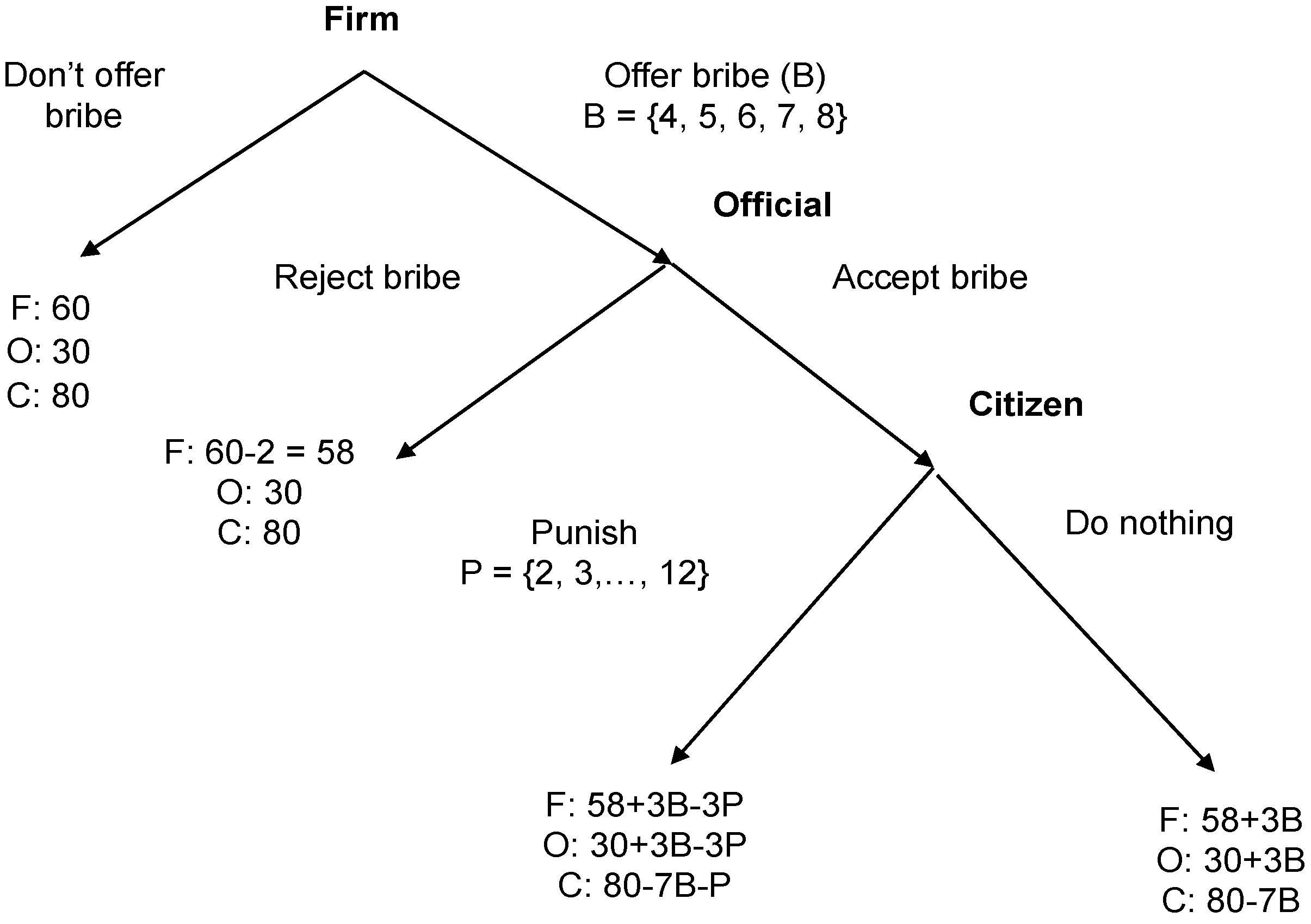
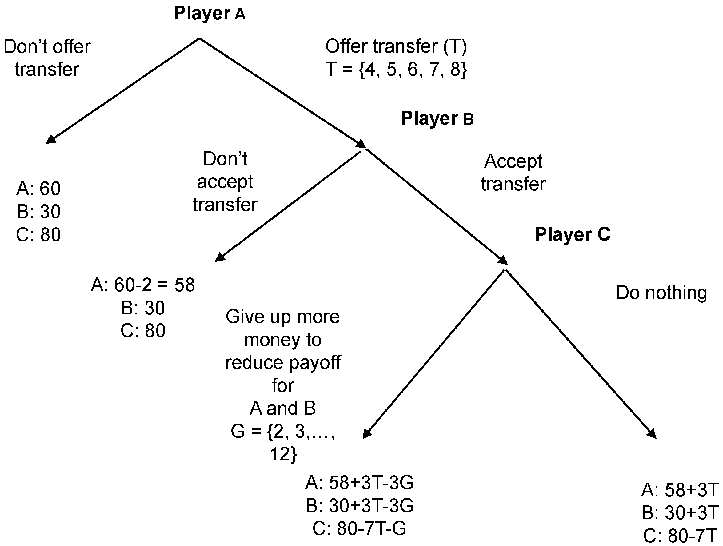
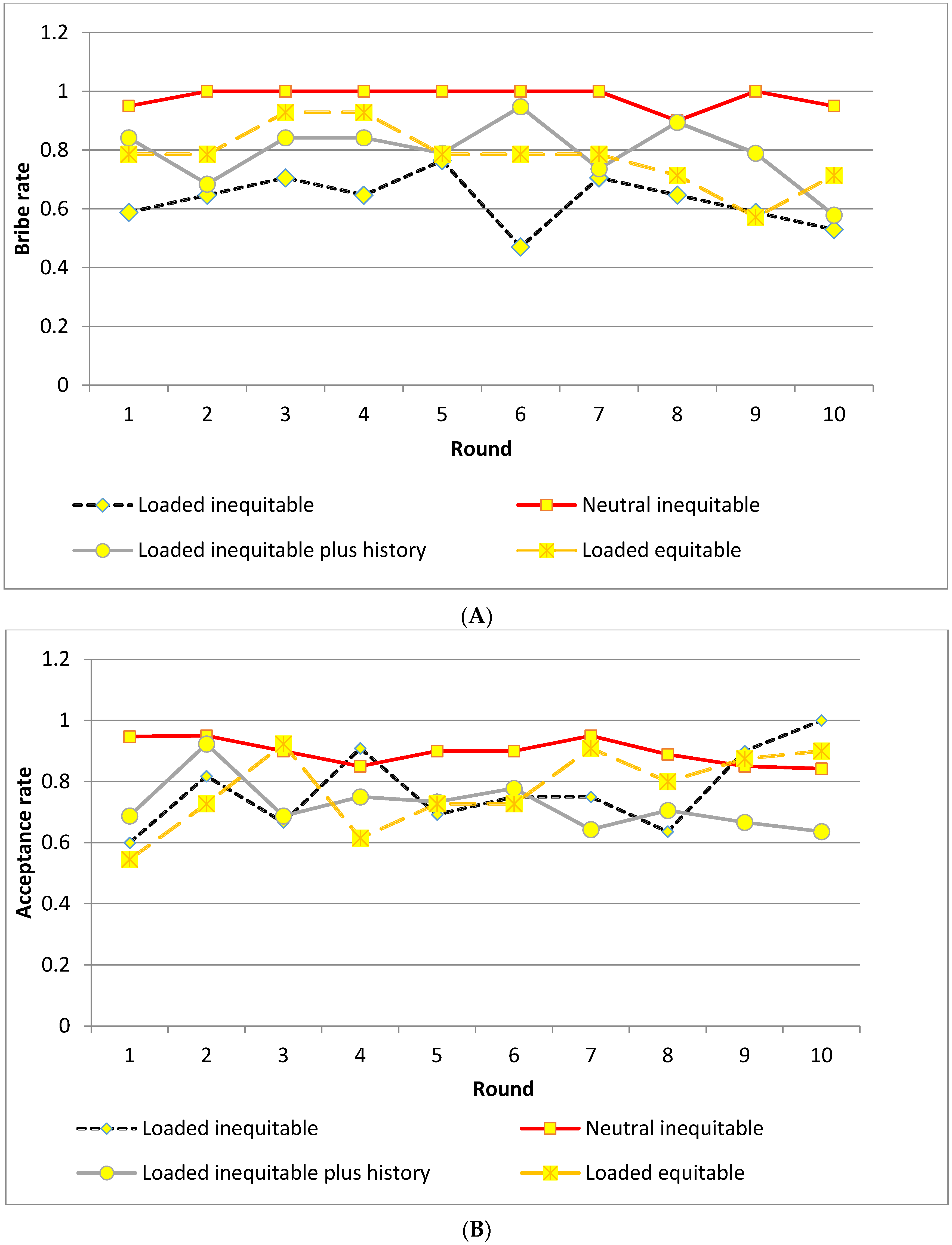
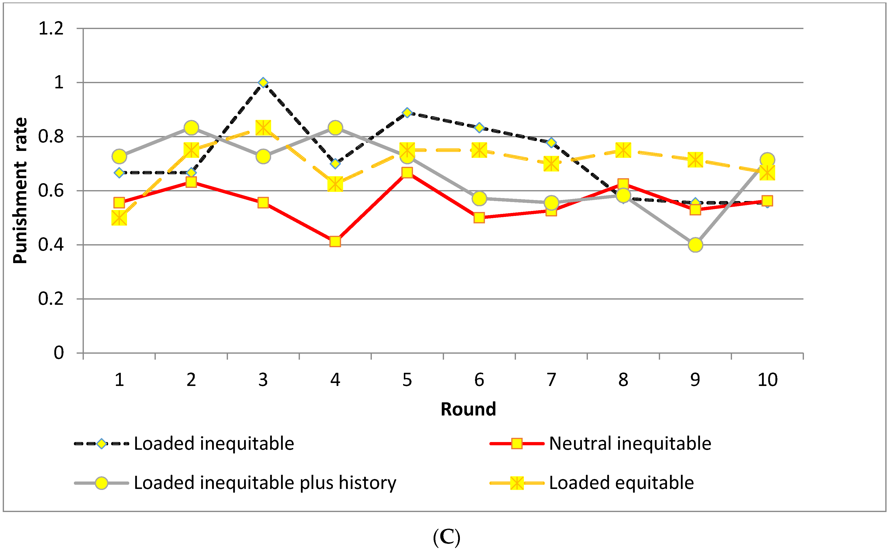
© 2016 by the authors; licensee MDPI, Basel, Switzerland. This article is an open access article distributed under the terms and conditions of the Creative Commons Attribution (CC-BY) license (http://creativecommons.org/licenses/by/4.0/).