2. The Model
Our description of the type of signaling game introduced by Lewis [
2] follows closely the equivalent and mathematically more convenient setup of Trapa and Nowak [
14]. A signaling game has two players, a sender and a receiver. A (pure) sender strategy can be represented as an
matrix
P. Each row of
P has one entry being equal to 1; all other entries are equal to 0. There are
n states of the world and
m signals. Each row of
P is associated with a state of the world and each column with a signal. If
, then the sender sends signal
j when state
i has occurred. Notice that
n may be unequal to
m, in which case the number of states is not the same as the number of signals.
Similarly, a (pure) receiver strategy will be represented by an matrix Q. A row of Q contains only zeros, except for one entry which is 1. Each row of Q is associated with a signal, while each column of Q corresponds to a state of the world (or, alternatively, one of n actions the receiver may perform). If , then the receiver associates state i with signal j (or chooses action i upon receiving signal j).
A mixed sender strategy (
, a convex combination of pure strategies) results in a stochastic
matrix
P;
,
for all
,
and
for all
. Analogously, a mixed receiver strategy results in a stochastic
matrix
Q. A stochastic matrix determines a behavior strategy [
9]. In the extensive form of a signaling game, each state of the world leads to a particular information set for the sender and each signal to one for the receiver. A stochastic matrix thus defines a behavioral strategy of a player,
, a probability distribution over choices at an information set. This representation of behavior strategies will become important when we consider evolutionary dynamics on behavior strategies (
cf.
Section 5).
The payoff function in a Lewis signaling game is given by
where
is the payoff to each player if their joint strategy is
. Hence, a Lewis signaling game is a partnership game, where both players get the same payoff for each outcome [
15]. This symmetry yields quite special best response properties. For convenience, we state a result from Pawlowitsch [
12] (
BR denotes the best-response correspondence).
Lemma 1. Let be a mixed sender strategy and be a mixed receiver strategy. If ,
then for all j moreover: analogous relations hold for sender strategies .
Lemma 1 implies that in order to find the maximum possible payoff given a certain strategy matrix, one just has to add its column maxima and normalize by .
A signaling game with
n states of the world and
n signals has
strict Nash equilibria, which have a very specific form; see e.g., [
14].
is a strict Nash equilibrium if and only if
P is a permutation matrix and
. Strict Nash equilibria represent states of perfect communication and are often called signaling systems [
2]. There are no strict Nash equilibria when the number of states is not equal to the number of signals [
14]. There exist non-strict Nash equilibria besides signaling systems, though. A partial characterization of Nash equilibria is given in Trapa and Nowak [
14]. If
B is an
matrix with no zero column, let us call
B uniform if there exist real numbers
, such that for each
j, the
j-th column of
B has 0 or
as entries.
Lemma 2. Let P be an sender matrix and Q be an receiver matrix and assume that neither P nor Q contains a zero-column. Then, is a Nash equilibrium iff P and Q are uniform and iff .
Hence,
(as subsets of
). Note that, at such a Nash equilibrium,
where the last equality follows from the fact that for each
i,
. Analogously,
and, thus,
.
Suppose that is a Nash equilibrium of the Trapa–Nowak class that is not strict. Then, it is clear that by continuous changes of the real numbers , , subject to the constraint that , the resulting profile will still be a Nash equilibrium. Hence, non-strict Nash equilibria of the Trapa–Nowak class are part of the components of Nash equilibria (and, therefore, never isolated).
As one of the
or
approaches 0,
P or
Q will have a zero-column. In this case, the assumptions of Lemma 2 are not met, and its conclusions do not hold. Pawlowitsch [
12] discusses these profiles at length. If signal
j is never sent by the sender, then the receiver can choose arbitrary probability weights
as long as the column maxima are preserved (this condition is necessary in order to preserve the best response correspondences of the players). Similarly, if the receiver never chooses state
i in response to any signal, then the probability weights
can take arbitrary values as long as column maxima are preserved.
As we already have noted above, signaling systems are the only strict Nash equilibria when . In order to single out plausible ones among the huge number of other Nash equilibria, we mitigate the concept of strict Nash equilibrium in two ways. It is clear that strict Nash equilibria in partnership games are strict local maximizers of the payoff function π. Let us call a strategy pair stable iff the common payoff function is locally maximal at , , for close to : . Such a strategy will be Lyapunov stable under many evolutionary dynamics, including the replicator dynamics.
It is well known that there is a one-to-one correspondence between strict Nash equilibria of asymmetric games and evolutionarily-stable strategies of their symmetrization (Selten’s theorem, see [
9]). Similarly, it follows that stable strategy pairs correspond to neutrally stable strategies of the symmetrization (see [
12] for definitions of neutral and evolutionary stability in signaling games). Therefore, we will refer to neutrally stable strategy pairs
also in the context of asymmetric games with the understanding that we really mean stable strategy pairs.
Pawlowitsch [
12] established the following important characterization of neutrally-stable strategies:
Lemma 3. Let P be an sender matrix and Q be an receiver matrix. Then, is neutrally stable iff P or Q has no zero columns, and neither P nor Q has a column with multiple maximal elements that are elements of the open interval .
Neutrally-stable strategies again give rise to components of Nash equilibria. Their significance derives from their role in the replicator dynamics of signaling games. For instance, neutrally-stable strategies are important for
when there are no strict equilibria. Then, the Pareto optimal component is asymptotically stable [
6]. However, as we will see below, they are also of crucial importance in the case
.
Another weakening of strict Nash equilibria that will turn out to be crucial for analyzing signaling games are quasi-strict Nash equilibria. In a two-player game, a Nash equilibrium is called quasi-strict if is contained in the simplex spanned by and is contained in the simplex spanned by . This means that there are no alternative best responses that are not contained in the faces spanned by x and y.
3. The Structure of Nash Components
In this section, we will try to get some more specific insights into the Nash equilibrium structure of signaling games. Knowledge of the geometry of Nash equilibria will prove to be particularly important once we start looking at the selection-mutation dynamics of signaling games.
We start with a useful general observation:
Lemma 4. In any partnership game, there are only finitely many Nash equilibrium payoffs.
Proof. Recall that if is a Nash equilibrium and p is a pure or mixed strategy for Player 1, whose support is contained in that of , then . Suppose now that and are Nash equilibria with the same support. Then, . The second equality follows since Player 2 has the same payoff function. Since there are only finitely many possible supports, there are only finitely many equilibrium payoffs. ☐
Therefore, even though the set of Nash equilibria may be infinite, the set of Nash equilibrium payoffs of a (finite strategy) partnership game is always finite. The reason is that along any continuum of Nash equilibria, the payoff function is constant.
Let us now determine the payoff levels of a signaling game with
at which Nash equilibria can be found. There are 6 strict Nash equilibria on the payoff level 1, given by a permutation matrix
P and
(these are the signaling systems). An example of this class is
The lowest payoff level at which Nash equilibria can be found is
. This payoff level includes Nash equilibria where the sender always uses the same signal or the receiver always chooses the same response. It also includes completely mixed equilibria, such as the barycenter. The
component is given by
where
and
. It follows from Lemma 2 that these are Nash equilibria. The
component is convex and invariant under permutations of strategies.
The Trapa–Nowak characterization of Nash equilibria assumes that strategy matrices contain no zero columns. However, there are Nash equilibria that do not satisfy this assumption. In the case of three signals, these additional equilibria can be found on the
and on the
payoff level. Strategy matrices on the former payoff level are of the form
with
, where
N can be a sender or a receiver matrix. These equilibria are all on the boundary of the component (3);
, they are limits of the strategy matrices (3).
At the payoff level
, there are Nash equilibria that are mixtures of signaling systems. An example is given by
Notice that Equation (
4) is isolated in the space of behavioral strategy profiles, but in the space of mixed strategies, it corresponds to a continuum of Nash equilibria. Each entry of
P or
Q can be realized by convex combinations of different pure strategies (in this case, eight pure strategies). Including permutations, the number of such mixed equilibria is 6.
The last, and most interesting, level is
. On the
level, there are equilibria, such as
with
. None of these Nash equilibria is neutrally stable (see Lemma 3). Note that the two-dimensional set of all these equilibria forms a Nash set [
16,
17]: every pair of such equilibria
is interchangeable,
,
and
are equilibria in this set, as well;
cf. [
18]. After renumbering events and signals, we obtain nine Nash sets like (
5). The interior equilibria
of these Nash sets (
, for
) are quasi-strict.
A typical neutrally stable strategy is given by
where
or
(
cf. Lemma 3 and Example 1 [
12]). All of these equilibria are also quasi-strict. When both
λ and
μ approach 0 or 1, these strategy pairs are still Nash equilibria, but no longer neutrally stable. The points on an edge (e.g.,
) are neutrally stable, but not quasi-strict. After permutations, we again obtain 9 two-dimensional Nash sets of this form.
Two more classes of Nash equilibria can be found on the
payoff level. One class is given by
with
. Strategies of type (
7) are not neutrally stable, because both
P and
Q have zero columns. Moreover, they are not quasi-strict (as shown in Proposition 8). There are 18 (two-dimensional) Nash sets of type (
7).
There is another class of neutrally-stable strategies that has, to our knowledge, not been noted in the literature before. A typical example is
where
and
. Notice that interior points in Nash sets such as (
8) are neutrally stable by Lemma 3. There are 18 (plus 18 more after interchanging the two players) three-dimensional Nash sets of type (
8).
Note that equilibria of the last two types are not limit points of Trapa–Nowak equilibria. Hence, not all Nash equilibria with zero columns are limit points of Nash equilibria whose strategy matrices contain no zero columns.
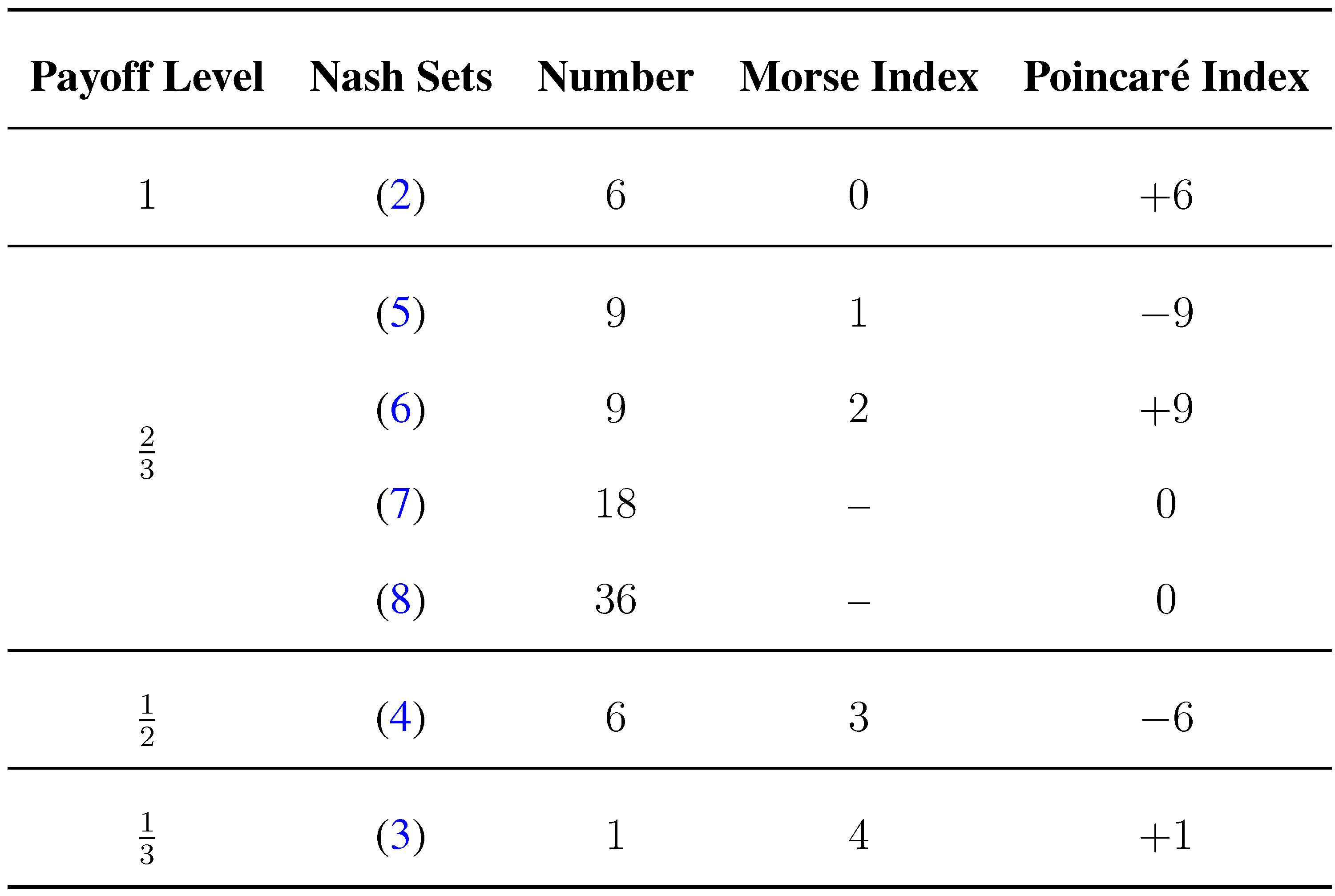
We provide an overview of the different types of Nash equilibria and their properties given in
Figure 1.
As we shall see in the next two sections, neutrally-stable strategies are of major importance from the point of view of evolutionary dynamics. Signaling systems are of course also neutrally stable by virtue of being strict Nash equilibria. As we have just seen, there are two other types of neutrally stable strategies besides signaling systems, namely strategy profiles (
6) and (
8).
Figure 1.
Summary for the Nash equilibria of a signaling game with
. The Morse index and the Poincaré index refer to the rest points of the selection-mutation dynamics in behavior strategies (14) for the case
. The Morse index is the number of positive eigenvalues of the Jacobian. At a maximizer of the potential function, the Morse index is 0. The Poincaré index is
if the number of positive eigenvalues is odd and
if it is even. The sum of the Poincaré indices is 1, which is equal to the Euler characteristic of the state space;
cf. [
15], Ch. 13.2.
There is an important difference between Nash sets, such as (
5), and Nash sets as given by (
6)–(
8). The two-dimensional Nash set (
5) is a subset of a larger polyhedron spanned by four sender strategies and four receiver strategies. The other Nash sets on the
payoff level are maximal in the sense that they contain no mixtures of pure strategies that are not included in the Nash set. Note that the
component is not convex (that it is connected will be shown in Proposition 7 below).
In the next proposition, we show that there are no Nash equilibria besides the ones listed above.
Proposition 5. In a signaling game with ,
is a Nash equilibrium iff belongs to one of the Nash sets of type (2)–(8). Proof. Let
belong to the Trapa–Nowak class of Nash equilibria. Suppose first that
for all
. Then, Lemma 2 implies that
belongs to class (
3).
Suppose now that one entry in a particular row is zero, e.g.,
(this can be achieved by renumbering the events and signals or interchanging the players) and that no entry of
P equals 1. Set
and
,
. If
, then
. Since
is the unique column maximum, this implies that
(Lemma 1), and from Lemma 2, it follows that
, a contradiction. Hence,
. If
, then
; and if
, then
. Assume the latter without loss of generality, and suppose
. Then,
by Lemma 2. Thus, either
or
, and, again, by Lemma 1,
or
, which implies that
. Thus,
, and we get
. Therefore, allowing one entry to be zero results in a Nash equilibrium belonging to class (
4).
A similar argument applies when we assume that one entry in one row is 1. If
, then
, and by Lemma 2,
. If
, then
, which contradicts the assumption that
P has a single entry 1. Therefore,
, and hence,
for
. Lemma 2 implies that
has the form (
5).
The argument in the last paragraph shows that assuming that one entry of
P equals 1 implies that the other two rows contain at least one zero. Nash equilibria of class (
6) result from the assumption that two entries in two rows equal 1. Indeed, if there are two entries in two rows that equal 1, then they must be elements of the same column by Lemma 2; e.g.,
(we are again assuming that
P is not a permutation matrix). If
, then
, a contradiction. Thus,
,
and
,
.
If we allow for three 1 entries (one in each row), then P is a permutation matrix, and by Lemma 2, . Hence, is a signaling system. This yields the last class of Trapa–Nowak Nash equilibria.
Other Nash equilibria have either two zero columns or one zero column. If there are two zero columns in, say,
P, then
is a Nash equilibrium if, and only if,
Q is as in (
3). The resulting Nash equilibria are part of the boundary of the set defined by (
3).
If, however,
P has only one zero column, then it looks like
The case
leads again to Nash equilibria belonging to the boundary of the component defined by (
3). Suppose
. Then, by Lemma 1, the maximum payoff against such a matrix is
. Hence, such a matrix is part of a Nash equilibrium only if
and
(
μ is arbitrary).
P is in Nash equilibrium with a strategy
Q, if and only if
belongs to the class of Nash equilibria given by (
7).
If
, then at a Nash equilibrium, we must have
and
. The best response to this strategy is constrained to look like the right-hand part of (
8). If
, then a similar argument leads again to Nash equilibria of type (
8).
This shows that if
is a Nash equilibrium, then it must belong to one of the classes (
2)–(
8). Applying Lemma 2 together with simple calculations shows that a joint strategy belonging to one of these classes is a Nash equilibrium. ☐
As an immediate consequence, we get information about the payoffs obtained in equilibrium. In a signaling game with three signals, all Nash equilibria are found on a specific payoff level. At a signaling system (
2), players earn a payoff of 1; at (
5)–(
8), players get
; at (
4), players get
; and at (
3), players get
.
The following proposition summarizes the number of each kind of Nash set, which can be calculated by using simple combinatorial arguments.
Proposition 6. In the signaling game with ,
there are 6 signaling systems and 6 Nash equilibrium components of type (4), 9 Nash sets of type (5), 9 Nash sets of type (6), 18 Nash sets of type (7), 36 Nash sets of type (8) and, finally, one component of type (3). Proof. It is clear that there are
signaling systems and one Nash set of type (
3). Nash sets of type (
4) are determined by the location of the three 0 entries, which cannot be in the same column or the same row. Thus, there are again
such Nash sets. Nash sets of type (
5) and (
6) are determined by the location of a 1 entry. In both cases, the 1 entry determines which entries must be equal to 0, respectively 1. There clearly are nine possible Nash sets of each of these types. Nash sets of type (
7) are given by the location of the zero column, of which there are 3 possibilities, and the location of the two 1 entries, which can vary in 6 possible ways. We thus have
sets of this type. For type (
8), we look again at the 1 entries. There are three 1 entries, two of which must be in the same column. For each choice of location for the third entry, there are two possible locations for the two in the same column. Hence, there are 18 different configurations. We have to double this number, because the same holds for the other player. ☐
As we have already remarked, the component is of particular importance, since it contains all neutrally stable strategies. We can, in fact, show that it is a component. Call two Nash equilibria x and y path connected if there is a continuous path ϕ of strategy profiles connecting x and y, such that every strategy profile on ϕ is itself a Nash equilibrium. The following proposition establishes that each pair of Nash equilibria which yields a payoff of is path connected (indeed, by a piecewise linear path).
Proposition 7. The Nash equilibria on the payoff level are path connected. Thus, the corresponding 72 Nash sets constitute a single component of Nash equilibria.
Proof. First, notice that each Nash set of type (
8) is path connected to a Nash set of type (
6), since the signaler part of the former is a pure strategy. Likewise, it is clear that Nash sets of type (
7) are connected to Nash sets of type (
5). Thus, it will suffice to show that: (i) Nash sets of type (
5) are connected; (ii) Nash sets of type (
6) are connected; and (iii) one type of (
5) and one of type (
6) are connected.
Nash sets of type (
5) can be identified by the column of the sender matrix
j, which has
for some
i and
for
. This follows from the special properties of Nash equilibria of the Trapa–Nowak class (see Lemma 2). For the same reasons, Nash sets of type (
6) can be identified by locating the column of the sender matrix
j, which has
for some
i and
for
. For Nash sets of type (
5), we will show that if
; then, the 1 entry can be moved horizontally to
,
and vertically to
and
, such that no changes lead to a strategy profile, which is not a Nash equilibrium. Horizontal moves are possible, because we can get from (
5) to certain neutral Nash sets (
6), which also shows that claim (iii) holds. Vertical moves are possible because of Nash sets of type (
7). By symmetry, connectedness is established for all other sender strategies and the corresponding receiver strategies, as well. Similar arguments will establish claim (ii).
We start with the strategy matrices
Suppose
and call the corresponding strategy pair
.
is in Nash equilibrium with all receiver matrices of the form
(
cf. (
7)). If
is the receiver strategy with
, then
and
are connected by a line of Nash equilibria. However,
is part of the neutrally-stable Nash set
where
. This establishes claim (iii). Moreover, from this neutrally-stable Nash set, we can move to a Nash set of type (
5), where
. To this end, set
and
, and apply arguments analogous to the ones above (using Nash sets of type (
7)) to move along a path of Nash equilibria to the Nash set
If we return to the Nash set given by (
9), we can apply the same kinds of arguments to move from the vertex where
to the neutrally stable Nash set given by
and from there to the Nash set
which has
. This shows that the 1 entry can be moved horizontally.
From the corner
, we can move on a path of Nash profiles to another Nash set of type (
5), which is given by
To do this, we just have to use the sender matrix (
10). This shows that we can get from a 1 entry in the first row to a 1 entry in the second row. Hence, it is clear that we can also get to
by using horizontal movements. Starting at the corner
one can show by using a similar kind of reasoning that moving to a Nash set of type (
5) with
is possible without ever passing through a strategy profile that is not a Nash equilibrium.
Concerning (ii), we have already shown in the first part of the proof that one can move the column with two 1 entries from the second to the third column by passing through Nash equilibria of types (
5) and (
7). Similarly from the corner of the profile (
11) with
, one can move to the profile
This shows that horizontal moves of the columns defining neutrally-stable sets are feasible. Vertical moves are feasible because of the profiles of type (
7). For instance, one can get from (
11) to
by moving through
All other claims are established in a similar manner. ☐
In the next two sections, we will make use of the concept of quasi-strictness. The following two results relate quasi-strictness to the Trapa–Nowak class of Nash equilibria. Concerning our use of the term ‘mixed strategy representative’, note that a mixed strategy is a convex combination of pure strategies. In signaling games, pure strategies are zero-one matrices. A stochastic matrix P generally corresponds to more than one mixed strategy (P determines a behavior strategy). Thus, if is a pair of sender and receiver strategies, then a mixed strategy representative of is a pair of mixed strategies corresponding to P and Q, respectively.
Proposition 8. If is a Nash equilibrium where both P and Q contain at least one zero-column, then no mixed strategy representative of is quasi-strict.
Proof. Suppose without loss of generality that and for . Suppose is like Q, except that . Then, by Lemma 1, is an alternative best response to P. However, since , there exists a pure strategy in that is not in . This implies that no mixed strategy representative of is quasi-strict. ☐
For
, this implies that Nash equilibria of class (
7) are not quasi-strict. Boundary equilibria of (
3) with a zero column for the sender and the receiver matrix are also not quasi-strict. However, consider
as in (
3), and set
. Then,
is not quasi-strict, since the sender strategy that sets
is an alternative best reply to
Q, which is not in the support of any mixed-strategy representative of
P. This shows that the converse of Proposition 8 does not hold in general.
Proposition 9. If is a Nash equilibrium of the Trapa–Nowak class, then any mixed strategy representative of is quasi-strict.
Proof. Since is a Trapa–Nowak Nash equilibrium, Lemma 2 implies that and . Thus, a pure strategy not in or cannot be an alternative best reply to Q or to P. ☐
For the case
, the only class of Nash equilibria where the two propositions above do not apply are given by (
8) whenever
Q has no zero column. To see when such Nash equilibria are quasi-strict, notice that
P is the unique best reply to
Q if
Q has no zero column and
. Moreover, by Lemma 1, a pure strategy best reply to
P has a 1 entry only at the possibly positive entries of
Q, given these constraints on
Q. Note also that the equilibria in the Nash set (
8) (except the pure ones) are neutrally stable according to Lemma 3. However, as noted above, if
, then
is neutrally stable, but not quasi-strict.
4. Dynamics for Mixed Strategies
Several of the results obtained in the previous section are useful when studying the evolutionary dynamics of signaling games. For infinite population models, signaling games were studied most thoroughly in the context of the replicator dynamics [
11,
12]. The main problem for understanding the robust features of the replicator dynamics arises from the fact that in signaling games there are linear manifolds of rest points. The replicator dynamics of signaling games is thus not structurally stable, and perturbations of the dynamics will typically result in qualitatively different dynamical behavior.
For this reason, Hofbauer and Huttegger [
13] investigated a natural perturbation of the replicator dynamics—the selection-mutation dynamics of Hofbauer [
19]—for signaling games with two signals. The selection-mutation dynamics for two populations is given by
where
and
describe the state of each population,
are the payoff matrices and
are small, uniform mutation parameters. If
, the selection-mutation dynamics coincides with the two-population replicator dynamics. We assume that
ϵ and
δ are of the same order as they go to zero;
, there exists a fixed
, such that
as
.
In the case of signaling games, it is shown in Hofbauer and Huttegger [
13] that the selection-mutation dynamics is a gradient system with respect to the Shahshahani metric. The corresponding potential function is given by
The first term on the right-hand side is the average payoff in the sender population, which equals the average payoff in the receiver population since . The logarithmic terms imply that rest points must be in the interior of the state space if . Because of the potential function, there can be no limit cycle in the selection-mutation dynamics of signaling games.
There are some important relations between the selection-mutation dynamics and the replicator dynamics. The first one implies that the Nash equilibria of the underlying game (which are also rest points of the replicator dynamics) give some information about the location of rest points of the selection-mutation dynamics (for a proof, see 13).
Proposition 10. If is a rest point of the two-population replicator dynamics, which is not a Nash equilibrium, then there exists no rest point for the selection-mutation dynamics (12) close to for sufficiently small .
Another result asserts the existence of rest points close to the strict equilibria of signaling games. A Nash equilibrium is regular if the Jacobian matrix J of (12) with has no zero eigenvalues, and it is hyperbolic if J has no eigenvalues with zero real part. Note that for partnership games, where , the replicator dynamics is a gradient, and hence, every regular equilibrium is hyperbolic. For such equilibria, a converse result to Proposition 10 holds.
Proposition 11. Let be a regular Nash equilibrium. Then, there exist unique rest point of the selection-mutation dynamics (12) close to for sufficiently small . Moreover, if is hyperbolic, then the perturbed rest point has the same stability properties under the selection-mutation dynamics as has for the replicator dynamics.
For proofs of Proposition 11, see Bürger and Hofbauer [
20], Ritzberger [
21], and, in the more specific context of signaling games, Hofbauer and Huttegger [
13]. For signaling games, Proposition 11 implies that there exists a unique family of asymptotically-stable rest points of the selection-mutation dynamics close to each signaling system whenever
are sufficiently small.
Regular Nash equilibria are isolated. As we have seen in the
case, there are no isolated Nash equilibria other than signaling systems. This means that Proposition 11 only applies to signaling systems. In particular, Propositions 10 and 11 do not determine the dynamical properties of the selection-mutation dynamics (12) close to neutrally-stable Nash sets, such as (
6). Neutrally-stable Nash sets are important in the replicator dynamics. As was shown in Pawlowitsch [
12], neutrally-stable Nash sets attract an open set of initial conditions under the replicator dynamics without being asymptotically stable sets (neutrally-stable Nash sets cannot be asymptotically stable since the vertices of the set are unstable). No general results apply in this case. It is therefore unclear what will happen close to these sets under the selection-mutation dynamics.
The rest of the present paper is devoted to the analysis of the selection-mutation dynamics for signaling games. Our analysis will rely heavily on the results obtained in the previous section. Some of the questions we are interested in will be investigated in the context of the selection-mutation dynamics as given by (12), , in the context of mixed strategy spaces. This framework does not seem to be suitable for other problems, since the dimension of the state space is too large. For signals, the state space of the selection-mutation dynamics (12) is a 52-dimensional polyhedron (there are 27 strategies for each player). It is thus very difficult to investigate the behavior of the selection-mutation dynamics close to Nash equilibria other than signaling systems. Therefore, in the next section, we will consider behavioral strategies. In particular, we will study the dynamic features in the neighborhood of neutrally-stable Nash sets in the context of selection-mutation dynamics for behavioral strategies.
Consider, for example, the Nash set given in (
5). For
, these equilibria belong to the Trapa–Nowak class of Nash equilibria. Therefore, by Proposition 9, Nash equilibria given by (
5) are quasi-strict as long as
. If we view these equilibria in terms of mixed strategies, they are located on the boundary region
M spanned by the product of the four sender strategies
with the four receiver strategies represented by the same matrices. Consider an equilibrium
in the relative interior of
M. Since
is quasi-strict, all transversal eigenvalues in (12) with
are negative [
9]. This implies that there exist orbits in the interior of
that approach
under the replicator dynamics. Hence, we may restrict our analysis of the stability properties of
to the replicator dynamics on
M. The set of Nash equilibria in
M consists of two signaling systems and a linear manifold of Nash equilibria
N corresponding to the mixed-strategy representatives of (
5). It is straightforward to show that the linearization of the replicator dynamics at
always has one eigenvalue with a positive real part. Hence, each
is linearly unstable.
Let us now consider the selection-mutation dynamics (12) close to N. Suppose there exist rest points of (12) close to points in the relative interior of N. Since the entries of the Jacobian matrix of (12) are continuous in , each rest point close to a point in the relative interior of N will have an eigenvalue with positive real part for sufficiently small . Such a perturbed rest point will thus be linearly unstable.
The same kind of reasoning applies to Nash sets of type (6). In this case, there are eight pure sender strategies and eight pure receiver strategies in the support of . If is an interior equilibrium of in the boundary region spanned by these strategies, then is linearly unstable. Thus, any rest point of (12) close to will also be linearly unstable for sufficiently small values of the mutation parameters.
This kind of reasoning can be generalized to signaling games with signals. The key fact is that there are always at least two signaling systems in the support of the mixed strategy representatives of the corresponding Nash sets.
Proposition 12. Let be a Nash equilibrium of the Trapa–Nowak class and a mixed strategy representative of , which has a signaling system in its support. Then, is linearly unstable if it is not a signaling system. Consequently, a rest point of (12) close to is linearly unstable for sufficiently small .
Proof. Let
J be the Jacobian matrix of the replicator dynamics evaluated at the point
. Since signaling games are partnership games,
J is a self-adjoint linear operator relative to the Shahshahani inner product,
,
for all
in the tangent space of the population state space;
cf. [
15], p. 259. Hence,
J has at least one positive eigenvalue if
J is not negative semi-definite. If we set
and
where
where
is a signaling system in
, then
(where
A is the payoff matrix corresponding to the signaling game); the inequality follows from the fact that
. This shows that
J is not negative semi-definite. ☐
Proposition 12 also applies to the Nash set of type (
3). For this component, we can actually show more. As was already observed in
Section 3, Equation (
3) is compact and convex. This also holds for its counterparts in signaling games with
[
11]. The average payoff is constant along this component. The potential function
V of (
13) will thus take on a unique maximum on this component.
An analysis of the Nash sets (
6)–(
8) is more involved, however. One reason for this is the fact that (unlike Nash sets of type (
3)–(
5)) these Nash sets do not contain mixtures of pure strategies that are not included in the Nash set; in particular, no signaling system is in their support.
Most equilibria in Nash sets of type (
6) are quasi-strict by Proposition 9. Thus, for the replicator dynamics, all transversal eigenvalues have a negative real part. The two remaining eigenvalues are zero. It is therefore
a priori unclear what will happen under the selection-mutation dynamics (12). Numerical calculations for specific mutation parameters
suggest that, in this case, there always exists a unique perturbed rest point close to each Nash set of type (
6), which is linearly unstable, having two positive eigenvalues. Hence, its Morse index is two (see
Figure 1 for a definition of the Morse index and the Poincaré index below). The same numerical procedures lead to the result that there are no perturbed rest points close to Nash sets of type (
7) and (
8); there are, however, unique perturbed rest points near each Nash set of type (
3)–(
5). The perturbed rest point close to the Nash set (
3) has four positive eigenvalues (Morse index four); perturbed rest points close to (
4) have three positive eigenvalues (Morse index three); and perturbed rest points close to (
5) have one positive eigenvalue (Morse index one). These calculations were conducted with several specific values for
ε close to zero.
These findings agree with index theory (Brouwer degree theory): the sum of the Poincaré indices of all (perturbed) rest points equals one, which is the Euler characteristic of
. (The Poincaré index is equal to
.) For the perturbed dynamics (12), the sum of the Poincaré indices of the six signaling systems and the six rest points close to the Nash set (
4) is zero; likewise, the sum of the Poincaré indices of the nine rest points close to Nash sets of type (
5) and the nine rest points close to the Nash set (
6) is zero, as well. The Poincaré index of the only remaining rest point is one. This information is summarized in
Figure 1.
In addition to these numerical results, a more thorough analytical treatment of the selection-mutation dynamics would be desirable in order to find out more about the stability properties of neutrally-stable Nash sets. Because of the many dimensions of the mixed strategy space for the
signaling game, such an analysis does not appear to be feasible for Nash sets of type (
6)–(
8). An analysis in terms of behavioral strategies is more promising.
5. Dynamics for Behavioral Strategies
The relationship between mixed strategies and behavioral strategies in extensive games of perfect recall is well understood [
22]. In particular, if one is interested in the equilibrium structure of extensive form games, then no essential information is lost by focusing on behavioral strategies. We propose a similar move for the evolutionary dynamics of signaling games.
The selection-mutation dynamics on the space
of behavioral strategies for signaling games is given by
where
The selection-mutation dynamics in behavioral strategies can be thought of as a dynamics in the entries of the sender and receiver matrices, since these matrices are nothing but a representation of the game’s behavioral strategies. Using (14) instead of (12) significantly reduces the dimensions of the state space. For , the mixed strategy space has effectively 52 dimensions, while the behavioral strategy space has only 12. For general the mixed strategy space has dimensions, whereas the space of behavioral strategies has . Moreover, it is easy to see that the Propositions 10 and 11 also hold for (14).
5.1. Replicator Dynamics
We begin by quickly reviewing some results for the replicator dynamics of signaling games, where the replicator dynamics is taken to be on behavior strategies;
, we are looking at (14) with
. The results we state follow immediately from the corresponding results for mixed strategies [
11,
12].
First of all, it is clear that signaling systems are asymptotically stable. Next, the Nash sets (
6) and (
8) are not asymptotically stable, but they attract an open set of initial conditions (they are attractive). This follows from the fact that all Nash equilibria in such a Nash set, except the vertices are neutrally stable and, hence, Lyapunov stable under the replicator dynamics [
12]. Straightforward calculations show that the transversal eigenvalues are negative, while the remaining eigenvalues are equal to zero. The center-manifold theorem then implies that the two types of Nash sets are attractive.
The other Nash sets are not attractive. They will be discussed in more detail in the following subsections. We start with the simple or less interesting cases, which include signaling systems and the Nash sets that are not even quasi-strict. We investigate the most interesting cases of neutrally stable Nash sets at the end of this section.
5.2. Signaling Systems
For , the location of perturbed signaling systems can be easily computed. The state with and for is the limit of a family of perturbed rest points of (14) as go to zero. We have , and hence, we obtain from (14) for , and to first order; so, and . The formulas for the other perturbed signaling systems are similar.
Since signaling systems are strict Nash equilibria, it is clear that perturbed signaling systems must be asymptotically stable for sufficiently small ; this follows from the continuity of the eigenvalues in ε and δ.
5.3. The 1/3 Component
As was noted above, the
component is convex. As in the case of mixed strategy evolutionary dynamics, it follows that there is a unique maximum of the potential function (
13) on this set. This determines a unique rest point of (14) in this set, which is given by
By continuity, this rest point must be linearly unstable. Calculating the eigenvalues of the Jacobian matrix of (14) at for shows that there are four zero eigenvalues, four positive eigenvalues and four negative eigenvalues. It follows that for small positive , the four zero eigenvalues become negative. Hence, the Morse index of the perturbed rest point is four.
5.4. Type (4) Rest Points
In terms of behavior strategies, this type of rest point is regular. It follows from the implicit function theorem that there exists a unique family of perturbed rest points of (14) close to (4) for sufficiently small
ε and
δ. By continuity, the perturbed rest point must be linearly unstable. In the dynamics (14) with
, the rest points of type (
4) have three positive rest points. Hence, the Morse index of the perturbed rest point is three.
5.5. Type (7) Nash Sets
Analyzing the dynamic behavior of (14) close to the other Nash sets requires more work. We start by considering Nash sets of type (
7). We are going to show that Nash sets of type (
7) do not persist under the selection-mutation dynamics (14). The intuitive reason for this is that these Nash sets are not quasi-strict; there always is a signaling system that is not used in the sender population. Introducing senders who utilize the unused signals and receivers who respond to it appropriately will destabilize any equilibrium in this set. Since such mutations will be introduced in the dynamics (14), no rest point of type (
7) can persist under selection-mutation dynamics.
Proposition 13. The behavior strategy given by with ,
is not the limit of a sequence of perturbed rest points. Analogous statements are true for the other Nash sets of type (7). Proof. Assuming the existence of perturbed rest point close to (
15), we can calculate the first-order expressions of the following variables,
and
Set
and
. Note that
, as
. Assuming the existence of a perturbed rest point, we must have
where
and
and
Hence
This system of equations has no solutions for sufficiently small
. To see this, notice that (16b) implies
and, hence, from (16a)
Therefore
which fails to hold as
. ☐
5.6. Type (5) Nash Sets
We now investigate the dynamics of (14) close to (
5). By a symmetric perturbed rest point, we shall mean a rest point that exhibits certain symmetry properties (the meaning of which will become clear below). It should be emphasized that there might be other rest points of (14) close to the corresponding Nash sets that are not symmetric.
Theorem 14. There exists a unique family of (symmetric) perturbed rest points that converges to the equilibrium from the Nash set (5), as .
To a first approximation, these perturbed rest points are given by Analogous statements are true for the other Nash sets of type (5). Proof. If it exists, a symmetric perturbed rest point has the form
For this to exist, the following system must have a solution for
:
The left-hand sides of these equations can be understood as a function
, where the components of
are given by the left-hand side expressions of (
18). We see that
. Let
M be the four-by-four matrix of partial derivatives of
F with respect to
evaluated at the point
. Then,
M is given by
Thus,
M is regular, and it follows from the implicit function theorem that there exist unique solutions for (
18) in terms of
ε and
δ provided that
are sufficiently close to zero. Indeed, linearizing the system (
18) at the point
gives
Hence, and , where stands for terms of order or higher. ☐
Points in the relative interior of Nash sets like (
5) have one positive eigenvalue under the replicator dynamics. Hence, the Morse index is one. It follows that each rest point in the family of rest points given in Theorem 14 is linearly unstable for small
. By considering the characteristic polynomial of the Jacobian of (14) evaluated at one of these perturbed rest points, we can obtain sharper results.
Theorem 15. Let be the perturbed rest point given by Theorem 14. Then, the following two statements are true for sufficiently small mutation rates: If , then the Jacobian matrix of the selection-mutation dynamics (14) is hyperbolic and has one positive eigenvalue.
If or , the Jacobian matrix of the selection-mutation dynamics (14) is hyperbolic and has two positive eigenvalues.
Proof. Calculating and factorizing the characteristic polynomial
of the Jacobian matrix evaluated at the rest point
of Theorem 14 yields four factors; up to higher order terms in
, a Taylor expansion around
yields the following approximations of the factors (up to multiplication by a positive constant):
Setting the first factor to zero yields two solutions for
x, which are given by (again up to higher order terms)
For all sufficiently small , one will be positive and the other one negative.
The eigenvalues given by the second and the third factor depend on
ε and
δ. By examining the discriminant of (21), it can be shown that the corresponding cubic equation has three solutions, which we will denote by
. Then
Now, setting to zero in the second factor of (21), and solving the cubic equation leads to three solutions for x, two of which are negative and one of which is zero (this last one is one of the zero eigenvalues of the replicator dynamics at this rest point). If are small, it follows that two solutions of must also be negative. Returning to (24), this implies that if , then . Conversely, if , then exactly one solution must be positive.
A similar argument leads to the same conclusions for the third factor of (22). In this case, if , then all eigenvalues coming from this factor are negative. If, on the other hand, , then one of the eigenvalues given by the third factor will be positive. Thus, from the second and the third factor, we get only negative eigenvalues if ; and we get exactly one positive eigenvalue if or .
The fourth factor can only yield negative eigenvalues. This can be seen by first setting and then solving the corresponding quartic equation for x. This yields four negative solutions, which will remain negative for (23) as long as are small. ☐
Example 16. The case
is especially important and was considered in the previous section within the context of the selection-mutation dynamics in mixed strategies. There, we observed that numerical calculations of eigenvalues of perturbed rest points close to (
5) yielded one positive eigenvalue. Theorem 15 is an analytical confirmation of this result, since if
, the clause of its first statement is fulfilled.
5.7. Neutrally-Stable Nash Sets of Type (6)
By far the most important alternatives to signaling systems are neutrally-stable strategies. In this section, as in the previous one, we first prove the existence of certain perturbed rest points close to Nash sets of type (
6) and then show that they will be linearly unstable under the selection-mutation dynamics.
Let us first note a simple observation concerning (
6). The next lemma asserts that if a point in the relative interior of a neutrally-stable Nash set is a limit of perturbed rest points, it must be the barycenter of the Nash set. Notice, however, that this result does not imply that there is at most one perturbed rest point close to a neutrally-stable Nash set. Several branches of curves of rest points might meet at the barycenter of the Nash set.
Lemma 17. Suppose that is a limit of perturbed rest points of the selection-mutation dynamics. Then, and .
Proof. If (25) is a limit of perturbed rest points, then approximate solutions up to higher order terms in
are given by
where
and
Since
,
and thus
The first term of the Taylor expansion in
of the left-hand side yields
Thus, if
, then
. A similar argument for
shows that if
, then
. Suppose
. Since
, we get:
The first term of the corresponding Taylor expansion is given by:
Thus, . By a similar argument, implies . Along the same lines, it can be shown that if . One just has to find the first terms of the corresponding Taylor expansions for and . ☐
We continue by proving the existence of certain symmetric perturbed rest points close to the two-dimensional Nash set (
6). Recall that we had some results concerning Nash sets of type (
5) for the selection-mutation dynamics in mixed strategies (12), whereas similar results for Nash sets of type (
6) were out of reach for the system (12).
Theorem 18. There exists a unique family of (symmetric) perturbed rest points that converges to the equilibrium from the Nash set (6), as .
To a first approximation, these perturbed rest points are given by Analogous statements are true for the other Nash sets of type (6). Proof. A symmetric perturbed rest point has the form
provided that it exists. It exists if the following system has a solution for
:
As in the case of the proof of Theorem 14, the left-hand sides of these equations can be understood as a function
, where the components of
are given by the left-hand side expressions of (27). We see that
. Let
N be the four-by-four matrix of partial derivatives of
G with respect to
evaluated at the point
.
N is given by
Thus,
N is regular and the implicit function theorem implies that there exist unique solutions for (27) in terms of
ε and
δ provided that
are sufficiently close to zero. Indeed, linearizing the system (27) at the point
yields
Hence, , , and , where denotes terms of order or higher. ☐
Next, we determine the stability properties and the Morse index of the rest point whose existence was proven immediately above.
Theorem 19. Let be the perturbed rest point given by Theorem 18. Then, the following two statements are true for sufficiently small mutation rates: If , then the Jacobian matrix of the selection-mutation dynamics (14) is hyperbolic and has two positive eigenvalues.
If or , the Jacobian matrix of the selection-mutation dynamics (14) is hyperbolic and has one positive eigenvalue.
Proof. By calculating and factorizing the characteristic polynomial
of the Jacobian matrix evaluated at the rest point of Theorem 18, we get four factors (we omit higher terms in
):
The first and the last factors only yield negative eigenvalues. This can be seen by first setting and then solving the resulting quadratic and the cubic equations. The solutions are negative and, thus, continue to be negative for small positive .
The eigenvalues given by the second and the third factor depend on
ε and
δ. Since the discriminant of (30) is positive, the corresponding cubic equation has three solutions, which we will denote by
. Then, in this case, we have
and thus
Now, setting to zero in the second factor of (30), and solving the resulting cubic equation leads to two negative solutions for x and another one where . If are small, it follows that two values among must also be negative. By (33), this implies that if , then ; and if , then exactly one solution must be positive. For the third factor of (31), it can be shown that if , then ; and if , then exactly one solution must be positive. In sum, the rest point has two positive eigenvalues, as long as , and one if one positive eigenvalue if or . ☐
Example 20. Consider again the example
. For the selection-mutation dynamics in mixed strategies, we noted in the last section that numerical calculations suggest that there exist unique rest points close to the barycenter of the Nash set (
6) that have two positive eigenvalues. Theorem 19 is an analytical confirmation of the latter point in the framework of behavioral strategies. If
, then the proviso of the first statement of the theorem clearly holds, and thus, the symmetric perturbed rest point has two positive eigenvalues.
Theorems 14 and 18 show that a family of (symmetric) perturbed rest points always exists close to Nash sets, such as (
5) and (
6). The existence of perturbed rest points does not depend on the ratio
. Their stability properties on the other hand do: while the symmetric perturbed rest points are linearly unstable for sufficiently small
regardless of the ratio
, the number of positive eigenvalues depends on it.
5.8. Neutrally-Stable Nash Sets of Type (8)
The ratio
is also relevant for the existence of perturbed rest points close to Nash sets of type (
8), to which we now turn our attention.
Theorem 21. Let with and .
Denote by those Nash equilibria in (34) with and .
If , then there are no perturbed rest points converging to as .
If , then there exists a family of perturbed rest points converging to some as .
If , then there exists a family of perturbed rest points converging to some as .
Proof. The Nash equilibrium (34) is quasi-strict, with
. Hence, to first order, a perturbed equilibrium nearby satisfies
and
For the remaining variables, we make an ansatz
with
small if
are small. Hence,
.
Inserting all this into the three equations
and letting
with
and
gives three equations for the ratio
and, hence, two equations between
.
Under the symmetry assumptions
,
, these two equations hold, and (36) reduces to
and thus
Hence, we obtain two disjoints intervals of solutions: for , we have , and for , we have . ☐
There are 18 Nash sets of the same structure as
(
P being a zero-one matrix). If we interchange
P and
Q, we obtain eighteen further Nash sets. In these cases,
ε and
δ switch roles in the proof of Proposition 21. Therefore, we have 36 perturbed rest points near Nash sets of type (
8) in cases 2 and 3 of the theorem. One can show that the perturbed rest points from case 2 have Morse index two, whereas those in case 3 have Morse index one. Hence, the total Poincare index of all 36 perturbed rest points is zero.


