An Equilibrium Analysis of Knaster’s Fair Division Procedure

Abstract

In an incomplete information setting, we analyze the sealed bid auction proposed by Knaster (cf. Steinhaus (1948)). This procedure was designed to efficiently and fairly allocate multiple indivisible items when participants report their valuations truthfully. In equilibrium, players do not follow truthful bidding strategies. We find that, ex-post, the equilibrium allocation is still efficient but may not be fair. However, on average, participants receive the same outcome they would have received if everyone had reported truthfully—i.e., the mechanism is ex-ante fair.

1. Introduction

This paper conducts an equilibrium analysis of a sealed-bid auction proposed by famed mathematician Bronislaw Knaster. This auction was designed to efficiently and fairly allocate multiple indivisible items and has played an important role in the early development of the fair division literature.1 As in standard auctions, players in Knaster’s auction simultaneously submit a bid for each of the items, where each item is allocated to the bidder who submitted the highest bid for that item. Unlike standard auctions, however, the winning bidder of each item compensates the losing bidders in the form of side payments.2 When players are truthful, Knaster’s process generates an efficient assignment of the indivisible items and side payments so that each person receives, in their view, a proportional outcome.3 This is a basic notion of fairness. The workings of auction are best introduced via a simple “inheritance” example.4

Suppose Ann, Bob, and Carol are heirs to an estate containing four indivisible objects , , , and . The heirs have an equal clam to the objects and are looking to “ fairly” divide these items using Knaster’s procedure. In particular, each heir submits a bid for each item. In the table below, we display bid vectors for the three heirs, the sum of these bids (or total reported value), and each bidder’s initial fair share—i.e., of their total reported value.

Knaster’s procedure allocates each item to the highest bidder and uses these bid vectors to determine side payments for each player. In particular, side payments are constructed so that each heir receives an equal “surplus” over their initial fair share.

Since items go to the high bidder, heir receives , heir receives , and heir receives items and . These items received create value for the recipient. The amount of value created above the initial fair share for the recipient is the bidder’s initial excess valuation. If we add up the initial excess values for the three heirs we get surplus. In this example, the surplus is 6000.

Next, we divide the surplus equally among the participants and add this amount to each participant’s initial fair share to compute an adjusted fair share. An individual’s side payment is their value received minus their total adjusted fair share.

In summary, Knaster’s procedure awards each of the items to the high bidder and the bidders “ pay” their final excess valuation (players with negative excess valuation receive a payment). Heirs leave the auction with value equal to their adjusted fair share. In the example, ends up with item 1 and pays $3700 to compensate the other two heirs, gets item 4 and receives $2700, receives items and and receives $1000. By construction, the side payment made by balances with the amounts paid to and .

Knaster’s procedure generates efficient proportional outcomes when the heirs report truthfully.5 Despite this nice property, Knaster’s auction is vulnerable to manipulation if the players have knowledge of one another’s preferences. Suppose, for instance, Heir B increases his bid for item 1 from $4000 to $9400. Each bidder still wins the same items, however ’s side payment (compensation) increases from to $2700 to $3900, which is a clear improvement for . Kuhn (1967) provides a similar example in his analysis of Knaster’s procedure and concludes by saying,

“ The numbers in this example have been chosen only to exhibit the advantages that can accrue to a player who falsely portrays his own valuations with a knowledge of the other player’s true valuations. It points up a clear need for an analysis of the strategic opportunities of this situation.”

It is unclear, however, if such manipulation could or would take place when bidder information is incomplete. We therefore seek to answer Kuhn’s call for strategic analysis of Knaster’s auction, but provide the analysis in an incomplete information setting. In Section 2, we model Knaster’s procedure as a sealed bid auction. In Section 3, we find equilibrium bidding strategies for the Bayesian game induced by Knaster’s auction. Welfare consequences of strategic behavior are explored in Section 4.

2. Knaster’s Fair Division Procedure

In this section, we formalize Knaster’s procedure as an auction.6 Let be a set of unrelated items to be allocated among heirs, whom we shall henceforth refer to as players. Each player assigns the value to item , for . The private values for each item are independently distributed according to cumulative distribution function with support , where the probability density function of by Individual values are private, but the distribution function for each item is known to all players. Last, since objects are unrelated, the value to a player of receiving multiple items is simply the sum of each item’s value.

Knaster’s procedure solicits bids from each player and uses this information to make an allocation decision. Specifically, each player submits a bid vector to a mediator who awards each item to the high bidder. Thus, player is awarded item if .7 Next, side payments are computed for each item as follows:

• First, each player ’s initial fair share of item (defined as -th of their reported value) is computed—i.e.,
• Second, surplus value for unit (defined as the difference between the high bid and the average bid) is computed—i.e.,
• Third, a player ’s adjusted fair share is computed from the bids. This is the player’s initial fair share of item plus an even share of the surplus—i.e.,
• Last, player ’s side payment for item is their reported value received (if they win the item) minus their adjusted fair share—i.e.,
  It is easy to verify that .8

This concludes the description of the mechanism. Note that our definition of initial fair share and surplus is for each item. If we sum up a player’s initial fair share (surplus) for each item, we arrive at that player’s total initial fair share (total surplus) as in the example found in the introduction. Player ’s payoff for the -th item as a function of submitted bids is therefore

Since Knaster’s auction can be analyzed item by item, a player’s total payoff is just the sum of the player’s payoffs from each individual item—i.e., .

3. Equilibrium

Knaster’s procedure is a mechanism that induces a Bayesian game between players. In this section, we find the Bayes–Nash equilibrium for this induced game in symmetric and increasing bidding strategies.

3.1. Knaster’s Procedure with a Single Object

We begin with a heuristic derivation of a Bayes–Nash equilibrium when only one object is being auctioned.

Suppose players follow the symmetric and increasing strategy . We consider player 1’s best response problem. Player 1 wins the object if he has the high bid—i.e., . He receives compensation if one of the other players is the high bidder. For instance, Player 2 wins if , , , ...., and . It is convenient to define the following functions:

The best response problem for player 1 is to choose a bid to maximize his expected payoff—i.e., to solve:

The first order condition for the problem is found using Leibniz’s Rule:

Since the function is symmetric in its last arguments and the partial derivative of is

the first order condition simplifies to:

(1)

In a symmetric Bayes–Nash equilibrium , which, after inputting into (1), combining terms and simplifying, yields:

Thus, we are left with the differential equation

(2)

In standard auctions, the boundary condition is used to solve the differential equation. However, in Knaster’s auction, this condition is not optimal. Fortunately, there is a unique value such that . At this value, the differential equation reduces to the expression . This is our boundary condition. The solution to Equation (2) is found to be

(3)

where is defined such that .9 It remains to show that strategy profile where every player follows (3) forms a Bayes–Nash equilibrium.

Proposition 1 Symmetric equilibrium strategies in the Bayesian game induced Knaster’s Fair Division Procedure with players and one object are given by (3).

Proof. We need to check that following is an equilibrium. First, it is easily checked that the bidding strategy is increasing and continuous. Second, a bidder will never want to bid above or below . Bidder 1, for instance, should not submit a bid . A bid equal to wins the item with probability one, thus increasing one’s bid only decreases bidder 1’s expected payoff. Similarly, Bidder 1 should not submit a bid . A bid equal to is guaranteed to lose the item with probability one (but win the compensation), so decreasing one’s bid only decreases 1’s expected payoff since it lowers the compensation. Finally, the expected payoff of bidder 1 whose type is but bids as if his type were is

Differentiating with respect to and simplifying the resulting expression yields:

Now setting we have

If , then . If , then . Hence, is maximized at . Therefore bidding truthfully according to is a best response.

Example 1 Suppose and each player ’s private value is distributed according to the uniform distribution—i.e., for and , then the equilibrium bidding strategy for each player is given by .10

The equilibrium bidding strategy prescribes over reporting when the player is less likely to win the item and more likely to earn compensation (i.e., when ), truth telling at , and for a player to shade his bid when more likely to win the item and less likely to earn compensation (i.e., ).

Figure 1. Equilibrium Bidding Strategy for u(0,1) and N = 2.

Figure 1. Equilibrium Bidding Strategy for u(0,1) and N = 2.

In general, the equilibrium bidding strategy prescribed in (3) recommends players shade their bids when their type is higher than the threshold type and to pad their bid when their type is lower than the threshold. This is intuitive. When a player is not likely to win the auction, he can gain compensation by increasing his bid. Similarly, a high type player who is more likely to win the item can gain by lowering his bid to reduce the compensation he must pay others. As in other auctions with shading/padding, there is a marginal benefit/cost to such actions—i.e., increasing one’s bid increases the probability a player will win the auction and decreasing one’s bid increases the probability a player will lose the auction. In the optimal bid, a player continues shading/padding until the marginal benefit falls short of the marginal cost.

3.2. Multiple Objects

Since the items are unrelated, we can treat each item independently when searching for the optimal bid. The next theorem follows immediately.

Proposition 2 Symmetric equilibrium strategies in the Bayesian game induced Knaster’s Fair Division Procedure with players and multiple objects are given by the vector valued bid function , where for , is defined as

whereeach is defined as the such that .

4. Welfare and Comparative Statics

Knaster’s auction was designed to achieve an efficient and proportional outcome when all players report their true valuations—i.e., allocations where the items ended up with the people who valued them the most and each player receives, in their estimation, at least -th of the item’s value. However, in equilibrium, bidders typically do not report truthfully. We now check to see if this behavior has welfare consequences.11

We are interested in the impact that strategic behavior has on the fairness and the efficiency of the equilibrium allocation. However, in an incomplete information environment, the notion of fairness is slightly ambiguous. Specifically, we need to clarify what information players have at the time they are evaluating the outcome or expected outcome. In particular, we need to know if the players are evaluating the outcome before they know their type (i.e., ex-ante) or evaluating the outcome after the auction is done (i.e., ex-post).12 While Knaster was clearly interested in the ex-post case, we mention some results from the ex-ante case, which is of interest. It is useful to define these notions in terms of general allocation rules.

Let be an allocation rule—i.e., a function that assigns to each realization of types a specific allocation, then the following properties are of interest:

Definition 1 The item assignment of an allocation rule is ex-post efficient if, for each realization of types, the object in the allocation prescribed is assigned to the player with the highest realized type for that object.

Definition 2 An allocation rule is ex-post proportional if, for each realization of types, after the allocation rule has been applied, each player with realized type gets a utility of at least .

Definition 3 An allocation rule is ex-ante proportional if, prior to observing types, each player ’s expected utility from his part of the allocation rule is greater than .

Knaster’s auction, when players follow truth telling strategies, is an allocation rule that satisfies all three of the above properties. However, we are interested in whether Knaster’s auction, when players follow equilibrium strategies.

Several welfare results are immediate. First, the ex-post assignment of the items in equilibrium is the same as when players report truthfully—i.e., the item assignment is ex-post efficient. This follows since equilibrium bidding strategies are increasing. Second, aggregate welfare is the same in equilibrium as it is under truth telling. This follows from the fact that the ex-post assignment of items is the same and that side payments always sum to zero. Third, although aggregate welfare is the same, there are bidders whose expected utility in equilibrium is smaller than their expected utility when everyone tells the truth. This is easily demonstrated when , where the type always prefers the truth telling outcome. The reason is intuitive. This player’s bid in equilibrium is his true value—i.e., . At the Bayes–Nash equilibrium, relative to the truth telling outcome, the player wins the object with the same probability, has to pay more in compensation if he wins (since types lower than bid above their value), and receives less in compensation if he loses (since types above bid below their value).13 In contrast, low and high types, relative to the truth telling outcome, are better off at the equilibrium outcome.

Our next result concerns ex-ante fairness— i.e., a player’s belief about the outcome he will receive in the auction before he knows his value. Denote the expected utility of a player with type in the truth telling and equilibrium outcomes by and respectively. Specifically, we show that, on average, there is no difference in the truth telling outcome and the equilibrium outcome. Since the truth telling outcome is known to be proportional, the expectation is that the equilibrium allocation must also be proportional.

Proposition 3 The equilibrium outcome of Knaster’s auction is ex-ante proportional. In particular, the expected difference in the truth telling outcome and the equilibrium outcome is zero—i.e.,

Proof. We illustrate the proof for , the general case is similar and is left to the reader. Since the probability of winning the item is the same in equilibrium as in truth telling, the expected difference in is just the expected difference in the side payments. By design, the transfers always sum to zero regardless of whether we are at the Bayes–Nash equilibrium or the truth telling outcome—i.e., and . Thus,

The expected difference is

The transfer function is symmetric—i.e., . So, the above equality can be re-written as:

This implies

Since we know the truth telling outcome is proportional, the result follows.

Example 2 Consider when types are uniformly distributed over the interval and there are only two bidders. Using the bidding strategies computed in Example 1, this difference simplifies to . From this expression we can see that high types and low types both prefer the outcome under strategic behavior whereas middle types prefer the outcome under truth telling. The expression is maximized at . In addition, the expected difference is

While this result is nice, Knaster was interested in ex-post fairness—i.e., the values people had after the auction was finished. Unfortunately, Knaster’s auction does not yield an ex-post proportional outcome in equilibrium as our next result demonstrates.

Proposition 4 The equilibrium outcome of Knaster’s auction is not ex-post proportional.

Proof. Suppose types are uniformly distributed over the interval and there are only two bidders. Specifically, let Player 1 have the type and Player 2 have the type . The symmetric equilibrium bid function, as given in Example 1, for each player is . So, Player 1’s bid is and Player 2’s bid is . Therefore, Player 1 wins the object and pays Player 2 a compensation of . The outcome results in a profit of , which is worse than the ex-post proportional outcome for Player 1 of

Proposition 4 is discouraging, but expected given the form of the equilibrium bid function.14 Our last result explores if competition might eliminate this negative feature of Knaster’s auction. In particular, we want to know whether the equilibrium bid functions converge to truth telling as the number of players increases. Why? If this were true, as it is in the first price sealed bid auction, we would know that in the limit Knaster’s auction is ex-post proportional. Alas, this is not the case. 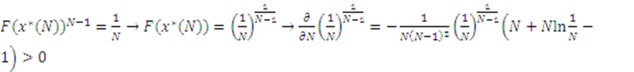The bid function in Knaster’s auction diverges from the 45 line as increases. To establish this claim, we demonstrate that the bid of the lowest type player is diverging from the truth as the number of players increases. First, however, we need the following lemma concerning the threshold type.

Lemma 1 Threshold type is strictly increasing in for .

Proof. if and only if . At , . Taking the derivative of the left hand side and right hand side yields and respectively. Now for , which implies . Thus, the right hand side is decreasing at a slower rate than the left hand side for all . So, for . Hence, is increasing in . Now is a cdf that , by assumption, is differentiable and strictly increasing. Thus, has an inverse that is strictly increasing. Thus, is also increasing in .

Now, we show that the bid function does not converge to the 45 line by demonstrating that the bid of the lowest type bidder is moving in the wrong direction.

Proposition 5 Equilibrium bid functions do not converge to the truth telling function as the number of bidders increases. In particular, the bid of the player with a type of zero, , is strictly increasing in for .

Proof. , where , , and .

The last equality follows from Leibniz’s rule and the fact that by definition of . Now from the chain rule:

Since we have . Thus, a sufficient condition for to be positive is for

Now since is less than or equal to we can form a bound on . In particular, the largest can get is

We now show .

The last inequality was established in Lemma 1. Therefore for all . It follows

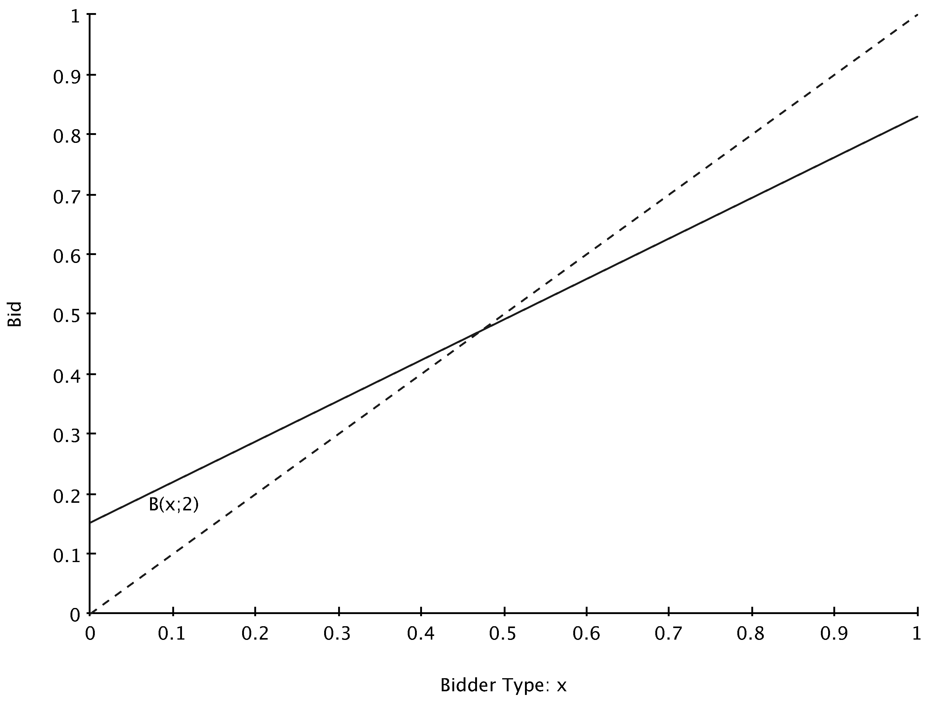
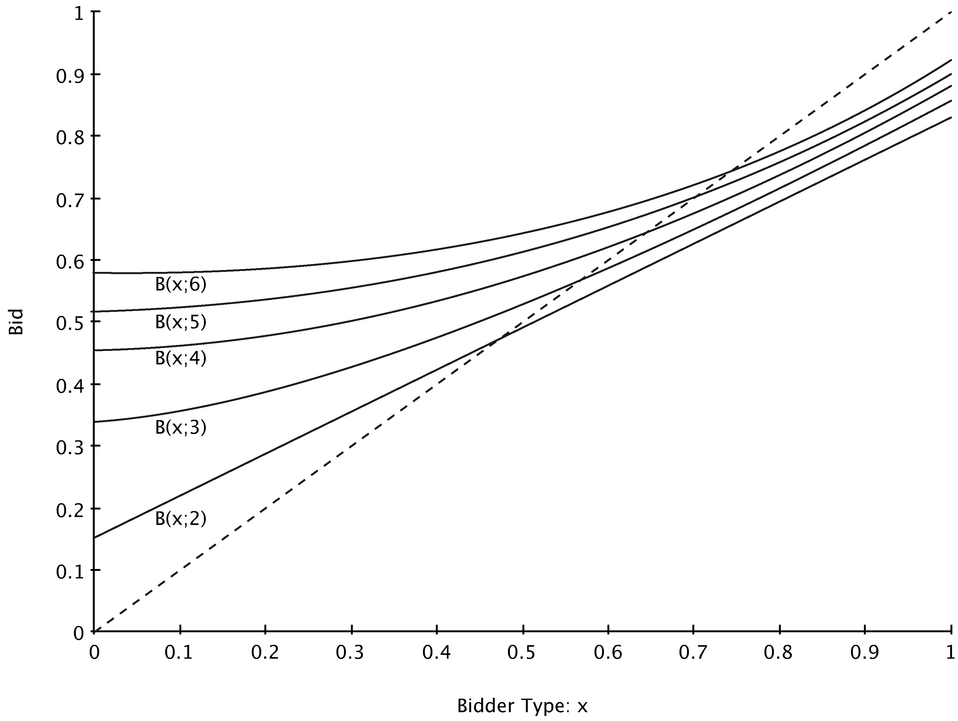
Example 3 The following diagram plots the graph of the bid function for the uniform distribution case when , , , , and . The bid functions displayed are each increasing in .

Figure 2. Bidding Strategies for u(0,1) N = 2,...,6.

Figure 2. Bidding Strategies for u(0,1) N = 2,...,6.

5. Discussion

The results in this paper contribute to several literatures: auctions, dissolving a partnership, bargaining, and fair division. In particular, we have used techniques frequently used in the auctions literature to analyze a well-known fair division procedure. Specifically, we have modeled Knaster’s fair division procedure as a sealed bid auction, computed the symmetric Bayes–Nash equilibrium in increasing bidding strategies, analyzed the welfare consequences of strategic behavior, and then performed some simple comparative statics of the equilibrium bidding functions.

Knaster’s auction remains efficient at the Bayes–Nash equilibrium outcome. However, the expected side payments made by bidders are typically different than under truth telling. As a consequence, the auction is no longer ex-post proportional.15 Additionally, since bidding strategies do not approach truth telling with competition, the distortions from truth telling created by strategic behavior do diminish with the number of players. However, despite these distortions, the auction does maintain some semblance of fairness. Specifically, the expected difference between the truth telling outcome and the Bayes–Nash equilibrium outcome is zero.

Fair division mechanisms, such as Knaster’s auction, are appealing when all individuals involved have a claim to an object or objects. Divorce, inheritance, and dissolving a partnership are natural contexts to apply such mechanisms. The later topic has been well studied in economics under the guise of efficiency when agents are strategic. Crampton, Gibbons, and Klemperer (1987), McAfee (1992), Morgan (2004), Moldovanu (2002) all study mechanisms for dissolving a partnership in an incomplete information environment.16 Specifically, Crampton, Gibbons, and Klemperer, working an independent private values framework, find a simple and efficient way to dissolve a partnership that is interim individually rational. This is in contrast to the well known impossibility theorem of Myerson and Satterthwaite.17 McAfee and Morgan’s papers are of interest to us because both papers consider fair division mechanisms. In particular, McAfee looks at an independent private values model and examines several simple auction mechanisms (including a simple cake cutting algorithm). In contrast, Morgan looks at several simple mechanisms in a two player common values setting and compares the outcomes of these mechanisms based on a fairness criterion. Clearly, Knaster’s auction could also be applied to any of these applied settings.

Brams and Taylor (1999) analyze the fairness properties of several simple fair division mechanisms and discuss how these procedures could be applied to bargaining scenarios.18 One of these mechanisms, the Adjusted Winner Procedure, for two players generates allocations that have several nice properties. Brams and Taylor (1996) compare Adjusted Winner with Knaster’s auction in several examples. Finally, we note that it is still an open question whether any of these mechanisms (or to what extent) are effective resource allocation mechanisms in practice. This question is well posed for future research.

6. Appendix

In this appendix, we provide the details for solving the differential equation (2). First, putting (2) in the standard form we have:

(4)

This can be solved using the integrated factor .19 Multiplying both sides of equation (4) by the integrating factor, we have:

Therefore, from the Fundamental Theorem of Calculus,

To dispense with the absolute value signs, we look at the function in two cases: and .

First, suppose , then by definition of absolute value . So, if , then

Now solving for the bid function yields:

Applying integration be parts, the last equation can be alternatively stated as

(5)

Second, suppose , then

Next, applying integration by parts on the two integrals on the right hand side of the equation gives us:

Solving for the bid function yields:

(6)

Finally, the two cases give us bidding functions (5) and (6). Applying the “initial” condition defines the constant of integration to be for both functions. The equilibrium bid function (3) is found by combining (5) and (9) and inserting the value of .

References

- Alkan, A.; Demange, G.; Gale, D. Fair allocation of indivisible goods and criteria of justice. Econometrica 1991, 59, 1023–1039. [Google Scholar] [CrossRef]
- Brams, S.; Taylor, A. Fair Division. From Cake Cutting to Dispute Resolution; Cambridge University Press: Cambridge, UK, 1996. [Google Scholar]
- Brams, S.; Taylor, A. The Win-Win Solution: Guaranteeing Fair Shares to Everybody; W.W. Norton and Company: New York, NY, USA, 1999. [Google Scholar]
- Crampton, P.; Gibbons, R.; Klemperer, P. Dissolving a partnership efficiently. Econometrica 1987, 55, 615–632. [Google Scholar] [CrossRef]
- Crawford, V. A game of fair division. Rev. Econ. Stud. 1977, 44, 235–247. [Google Scholar] [CrossRef]
- Crawford, V.; Heller, P. Fair division with indivisible commodities. J. Econ. Theory 1979, 21, 10–27. [Google Scholar] [CrossRef]
- Crawford, V. A self-administered solution of the bargaining problem. Rev. Econ. Stud. 1980, 47, 385–392. [Google Scholar] [CrossRef]
- Demange, G. Implementing efficient egalitarian equivalent allocations. Econometrica 1984, 52, 1167–1178. [Google Scholar] [CrossRef]
- Dubins, E.; Spaniers, E. How to cut a cake fairly. Am. Math. Mon. 1961, 68, 1–17. [Google Scholar] [CrossRef]
- Guth, W.; van Damme, E. A comparison of pricing rules for auctions and fair division games. Soc. Choice Welfare 1986, 3, 177–198. [Google Scholar] [CrossRef]
- Krishna, V. Auction Theory, 2nd ed; Academic Press: Waltham, MA, USA, 2010. [Google Scholar]
- Kuhn, H. On games of fair division. In Essays in Mathematical Economics in Honor of Oskar Morgenstern; Shubik, M., Ed.; Princeton University Press: Princeton, NJ, USA, 1967; pp. 29–37. [Google Scholar]
- Luce, D.; Raiffa, H. Games and Decisions: Introduction and Critical Survey; Wiley: New York, NY, USA, 1957. [Google Scholar]
- McAfee, R.P. Amicable divorce: Dissolving a Partnership with Simple Mechanisms. J. Econ. Theory 1992, 56, 266–293. [Google Scholar] [CrossRef]
- Moldovanu, B. How to Dissolve a Partnership. J. Inst. Theor. Econ. 2002, 158, 66–80. [Google Scholar] [CrossRef]
- Morgan, J. Dissolving a partnership (un)fairly. Econ.Theory bf 2004, 24, 909–923. [Google Scholar] [CrossRef]
- Moulin, H. Axioms of Cooperative Decision Making; Cambridge University Press: New York, NY, USA, 1988. [Google Scholar]
- Moulin, H. Fair Division under joint ownership: Recent results and open problems. Soc. Choice Welfare 1990a, 7, 149–170. [Google Scholar] [CrossRef]
- Moulin, H. Uniform externalities: Two axioms for fair allocation. J. Public Econ. 1990b, 43, 305–326. [Google Scholar] [CrossRef]
- Moulin, H. Fair Division and Collective Welfare; The MIT Press: Cambridge, MA, USA, 2003. [Google Scholar]
- Raiffa, H. The Art and Science of Negotiation; Harvard University Press: Cambridge, MA, USA, 1982. [Google Scholar]
- Robertson, J.; Webb, W. Cake-Cutting Algorithms: Be Fair if You Can; AK Peters: Natick, MA, USA, 1998. [Google Scholar]
- Segal, I.; Whinston, M.D. A simple status quo that assures participation (with application to efficient bargaining). Theor. Econ. 2011, 6, 109–125. [Google Scholar] [CrossRef]
- Su, F. Rental harmony: Sperner’s lemma in fair division. Am. Math. Mon. 1999, 106, 930–942. [Google Scholar] [CrossRef]
- Steinhaus, H. The problem of fair division. Econometrica 1948, 16, 101–104. [Google Scholar]
- Takenuma, K.; Thomson, W. The fair allocation of an indivisible good when monetary compensations are possible. Math.Soc. Sci. 1993, 25, 117–132. [Google Scholar] [CrossRef]
- Varian, H. Equity, envy, and efficiency. J. Econ. Theor. 1974, 9, 63–91. [Google Scholar] [CrossRef]
- Young, H.P. Equity: In Theory and in Practice; Princeton University Press: Princeton, NJ, USA, 1994. [Google Scholar]
© 2013 by the authors; licensee MDPI, Basel, Switzerland. This article is an open-access article distributed under the terms and conditions of the Creative Commons Attribution license (http://creativecommons.org/licenses/by/3.0/).
Share and Cite
Van Essen, M. An Equilibrium Analysis of Knaster’s Fair Division Procedure. Games 2013, 4, 21-37. https://doi.org/10.3390/g4010021
Van Essen M. An Equilibrium Analysis of Knaster’s Fair Division Procedure. Games. 2013; 4(1):21-37. https://doi.org/10.3390/g4010021
Chicago/Turabian StyleVan Essen, Matt. 2013. "An Equilibrium Analysis of Knaster’s Fair Division Procedure" Games 4, no. 1: 21-37. https://doi.org/10.3390/g4010021
APA StyleVan Essen, M. (2013). An Equilibrium Analysis of Knaster’s Fair Division Procedure. Games, 4(1), 21-37. https://doi.org/10.3390/g4010021