Carbon Border Adjustment and Strategic Environmental Quality: Quality Backfire and Market Contraction

Abstract

We develop a two-stage game with vertically differentiated products and endogenous environmental quality to study unilateral carbon pricing and the Carbon Border Adjustment Mechanism (CBAM). A home EU firm and a foreign exporter choose environmental quality, then compete in prices. Under unilateral pricing, only the home firm is taxed, so the foreign exporter’s quality choice responds only indirectly through competition, not a direct tax-saving motive. CBAM corrects this by taxing imports, too. We show that this correction can defeat itself: the same charge that incentivizes upgrading also contracts the foreign firm’s margin and market share, and once the carbon price exceeds a parameter-dependent threshold, this contraction can dominate, leaving the firm choosing lower quality under CBAM than under unilateral pricing. We analytically show that, sufficiently close to free trade, the foreign firm’s equilibrium quality is higher under CBAM than under unilateral pricing, so quality backfire is a finite-carbon-price equilibrium reversal rather than a local artifact, and numerically show that the reversal occurs over a substantial part of the admissible parameter region and survives several robustness checks. A second channel, where CBAM narrows the quality gap, could increase aggregate emissions, but the backfire is not realized in our calibration. The results provide a game-theoretic explanation of how border carbon policies shape strategic quality competition in carbon-intensive trade.

1. Introduction

Carbon pricing has become the central instrument of contemporary climate policy, and the European Union has pushed it furthest. On 1 January 2026, the Carbon Border Adjustment Mechanism (CBAM) entered its definitive phase, becoming the first large-scale operational border carbon adjustment to charge importers for embodied emissions in carbon-intensive goods such as cement, steel, aluminum, and fertilizers (European Commission, 2023). The stated rationale is twofold: to halt carbon leakage as free ETS allowances are phased out, and to level the competitive playing field between regulated domestic firms and unregulated foreign rivals (Bellora & Fontagné, 2023; European Commission, 2023). The policy’s logic is intuitive: if only domestic producers face a carbon charge, unregulated foreign rivals receive no direct carbon-pricing incentive to clean up their production, and may even have a strategic incentive to compete more aggressively on price using dirtier technology. CBAM closes this gap by extending the domestic carbon price to imports.

This paper asks a question that the policy design itself does not answer: does giving the foreign firm the same carbon incentive as the domestic firm actually translate into the foreign firm choosing cleaner technology? We show that the answer can be no, and for a reason that is specific to imperfectly competitive markets rather than to any flaw in the carbon-pricing logic itself. The same charge that gives the foreign exporter a direct incentive to invest in environmental quality also raises its marginal cost, which contracts its equilibrium price-cost margin and market share. Because the return to quality investment is earned over that margin and that market share, a sufficiently strong contraction can outweigh the direct tax-saving incentive CBAM was designed to create. The result is a foreign firm that ends up less clean under CBAM than it would have been under unilateral EU carbon pricing—not because CBAM fails to tax the foreign firm’s emissions, but because taxing those emissions changes the competitive environment in which the firm decides how clean to be. We call this the quality-backfire result. In the numerical analysis, it emerges beyond a parameter-dependent threshold and becomes more pronounced as the foreign firm’s quality-cost disadvantage or baseline emissions intensity increases.

A second and conceptually distinct concern arises once environmental quality is allowed to affect product differentiation itself. By inducing the foreign firm to upgrade, CBAM can narrow the quality gap between the two firms, intensifying price competition, expanding the overall size of the market, and potentially raising aggregate emissions even as each unit produced becomes cleaner. We characterize this aggregate-emissions channel analytically and derive the exact condition under which it would dominate the direct improvement in emissions intensity. This channel is conceptually important and threshold conditions are not generically empty, but in our calibrated analysis it is not the operative force: the market-expansion condition needed to generate aggregate backfire is demanding, and the dominant effect of CBAM in the numerical exercise is to contract the size of the market it regulates. The paper’s main quantitative result is, therefore, the quality-backfire result, not the aggregate-emissions channel, and we are explicit throughout about which of our results are demonstrated numerically and which remain theoretical threshold conditions describing when a mechanism could operate.

Whether CBAM achieves its objectives depends on how foreign firms actually respond, and the standard policy debate has been surprisingly narrow on this point. Much of the applied literature treats firms as passive: leakage is modeled as a relocation or output-reallocation effect within computable general-equilibrium frameworks (Böhringer et al., 2016, 2018), while the firm’s technology is held fixed. Yet the goods covered by CBAM are precisely those for which producers can, and increasingly do, choose how clean to be. Environmental quality is, therefore, a strategic decision variable, not a parameter, and it is chosen in anticipation of how rivals price and how regulators tax. This is the margin our paper places at the center of the analysis.

We formalize this mechanism in a multi-stage game of international competition with vertically differentiated products and endogenous environmental quality, building on the canonical quality-competition framework of Mussa and Rosen (1978) and Shaked and Sutton (1982). Two firms compete in the EU market. In the baseline model, a cleaner home firm and a dirtier foreign exporter differ only in the cost of producing environmental quality, with the foreign firm facing the higher quality-cost curvature.1 Taking the EU carbon-pricing regime as exogenously given, firms first choose environmental qualities and then compete in prices. We solve the pricing subgame in closed form, characterize quality choices through exact first-order conditions, and derive local sign characterizations of firms’ quality responses to a higher carbon price, supplemented by sharper analytical results in a tractable symmetric-emissions benchmark. We then use numerical analysis to evaluate the foreign firm’s quality response under unilateral pricing versus CBAM, and separately, the four margins that determine whether the aggregate-emissions channel is active: quality-gap narrowing, emissions-intensity reduction, market-coverage expansion, and total emissions change.

Our contribution is the following. First, we develop a vertically differentiated quality-price game in which environmental quality is chosen strategically before price competition, so carbon policy is studied not only as a cost shock, but also as a factor that reshapes firms’ product positioning. Second, we show that CBAM’s own corrective mechanism can undermine itself: the import carbon charge that gives the foreign firm a direct incentive to upgrade also weakens the margin and market share through which that incentive is realized. Furthermore, once the carbon price exceeds a parameter-dependent threshold, this can leave the foreign firm choosing lower environmental quality than under unilateral pricing alone. We establish analytically that, sufficiently close to free trade, the foreign firm’s equilibrium quality is higher under CBAM than under unilateral pricing, so quality backfire necessarily represents a finite-carbon-price reversal of the initial equilibrium response, and show numerically that this finite-carbon-price reversal occurs over a substantial part of the admissible parameter region and persists under the reported production-cost and several incomplete-CBAM robustness checks. Third, we identify an independent CBAM-specific channel through which narrowing the quality gap could expand market coverage and raise aggregate emissions even as average emissions intensity falls; we derive the exact threshold condition for this channel to dominate, but show it is not realized in our calibration, where CBAM instead reduces emissions mainly through market contraction. The two channels are analytically distinct, and only the first is numerically demonstrated. Finally, we complement the firm-level and emissions results with an EU and global welfare comparison, which separates the environmental consequences of CBAM from its distributional effects across consumers, domestic producers, the foreign exporter, and carbon revenues.

Three implications for policy follow. First, the diagnostics currently used to judge border carbon adjustment are not sufficient. Aggregate emissions in the regulating market and the size of the cross-border carbon-price gap can both move in the intended direction while the regulated foreign producer’s technology moves against it; a monitoring framework built on the first two indicators will not detect the third. Second, the design margins that matter are those that determine how much of the exporter’s margin the charge absorbs, like coverage ratios, crediting of foreign carbon payments, and the treatment of high-baseline-intensity exporters, rather than the headline equalization of the carbon price itself. Our robustness analysis shows that partial coverage can preserve foreign upgrading even when full coverage produces backfire, which is an uncomfortable finding for a policy whose stated goal is complete equalization. Third, the welfare and environmental evaluations need not coincide. In our calibration, CBAM raises EU welfare even at a zero social cost of carbon, since it leads to higher domestic profit and EU carbon revenue, which more than offset the loss in consumer surplus. Trade regulators evaluating border carbon adjustments proposed by other jurisdictions should, therefore, keep in mind that a domestic welfare gain should not by itself be interpreted as evidence of environmental effectiveness.

The remainder of the paper is organized as follows. Section 2 reviews the related literature. Section 3 sets up the model, derives the Bertrand pricing equilibrium and the quality-stage conditions, and presents the analytical comparative statics for unilateral pricing and CBAM. Section 3 also develops the emissions-decomposition result that identifies the differentiation-collapse channel through which CBAM may backfire at the aggregate level. Section 4 presents the numerical analysis and robustness exercises. Section 5 examines the welfare implications of CBAM relative to unilateral pricing. Section 6 discusses the results in relation to the existing literature and their policy implications, and concludes.

2. Literature Review

Our paper connects two strands of research: the economics of carbon leakage and border adjustment and vertical product differentiation with environmental quality. Each of these studies is extensive; for brevity, we discuss only the contributions most directly related to our mechanism, namely the interaction between carbon-pricing asymmetry, strategic firm behavior, environmental quality choice, and market coverage. We treat strategic trade-policy models under oligopoly briefly, as a motivating but methodologically distinct literature.

Carbon leakage and border carbon adjustment. The intellectual case for border adjustment builds on the trade-and-environment literature, including Markusen (1975) and Copeland and Taylor (1994, 1995), which showed how differences in environmental regulation can reallocate pollution-intensive activity across jurisdictions, the mechanism underlying modern leakage concerns. A large applied literature has since quantified leakage and evaluated border-adjustment designs, typically in multi-region computable general-equilibrium frameworks comparing border charges, export rebates, and output-based rebating (Bellora & Fontagné, 2023; Böhringer et al., 2016, 2018; Clausing & Wolfram, 2023; Fischer & Fox, 2012; Monjon & Quirion, 2011). This literature evaluates how border adjustment affects trade flows, emissions, and competitiveness at the sector or country level, but treats firm technology as fixed; Böhringer et al. (2022) confirm that this fixed-technology assumption substantially constrains the estimated environmental effectiveness of border carbon adjustments. We share Böhringer et al. (2016)’s emphasis on strategic responses to border policy, but relocate it from the nation-state to the firm and from quantity reallocation to endogenous quality choice, which lets CBAM affect aggregate emissions through the equilibrium quality gap and market coverage as well as through emissions intensity. Fontagné and Schubert (2023) provide a comprehensive survey of border carbon adjustment design, rationale, and distributional impacts. Ambec et al. (2024) study three carbon leakage mitigation instruments, namely free allowances, CBAM, and output-based rebating, in a trade model with endogenous emissions abatement. However, unlike the present paper, their framework does not treat abatement as a strategic quality variable chosen in anticipation of price competition. A closely related recent contribution is Fikru et al. (2025), who study optimal decarbonization policy when firms choose carbon capture and storage endogenously in a sequential game. Like us, they treat environmental outcomes as equilibrium responses to policy rather than as fixed parameters. The key difference is that Fikru et al. (2025) endogenize the policy instrument and model abatement as investment in capture technology, whereas we take the carbon-pricing regime as given and model environmental quality as a vertically differentiating product attribute chosen before Bertrand price competition. This linkage between environmental quality and product-positioning generates our quality-backfire mechanism.

A related strand studies environmental policy as strategic trade policy under oligopoly, drawing on the rent-shifting logic of Brander and Spencer (1985): governments may weaken environmental standards or taxes to confer a cost advantage on domestic Cournot producers (Barrett, 1994; Conrad, 1993; Kennedy, 1994; Rauscher, 1994; Ulph, 1996). We retain this literature’s strategic-interaction insight but relocate it from government standard-setting under Cournot competition to firm-level quality choice under Bertrand price competition over vertically differentiated goods, which generates the downgrading channel absent from quantity-based treatments.

Vertical differentiation and environmental quality. Methodologically, the paper builds on the theory of vertical product differentiation, pioneered by Mussa and Rosen (1978), Gabszewicz and Thisse (1979), and Shaked and Sutton (1982), and extended by Ronnen (1991) and Motta (1993). These models characterize markets in which consumers agree on the quality ranking but differ in willingness to pay, yielding the natural-oligopoly and price-competition results we exploit. A subsequent literature reinterprets “quality” as environmental quality and asks how taxation interacts with it: Cremer and Thisse (1999) and Lombardini-Riipinen (2005) study optimal taxation of a polluting quality attribute. Arora and Gangopadhyay (1995), Bansal and Gangopadhyay (2003), and Moraga-González and Padrón-Fumero (2002) extend this literature by exploring voluntary overcompliance and policy design with environmentally conscious consumers. Our innovation relative to this literature is to introduce an asymmetric, jurisdiction-specific carbon price, which is the defining feature of unilateral pricing versus CBAM, and trace its effect on the equilibrium configuration of qualities chosen by a domestic and a foreign firm. We show that equalizing the carbon charge can still lower the foreign firm’s environmental quality by contracting the market return to quality investment.

3. Model

3.1. Environment, Variables, and Parameters

We consider a vertically differentiated duopoly in which two firms compete in the European market. Firm H (home, EU) supplies the higher-quality, cleaner variety, while firm L (foreign) supplies the lower-quality, more polluting variety.

Consumers are indexed by $\theta \sim U[0,1]$, representing willingness to pay for environmental quality. Utility from purchasing product $i\in \{H,L\}$ is

$$U_i\left(\theta \right)=\theta A_i-p_i,$$

(1)

where $A_i$ denotes environmental quality and $p_i$ is price. The outside option yields zero utility.

We assume vertical differentiation,

$$A_H>A_L>0.$$

(C1)

Variables and parameters.

• $A_i$: environmental quality of firm i
• $p_i$: price of firm i
• $x_i$: demand for firm i
• $e_i\left(A_i\right)$: emissions per unit
• ${\rho }_i$: effective per-unit carbon charge in the EU market
• ${\gamma }_i$: curvature of quality cost
• $a_i$: baseline emissions parameter
• $b>0$: emissions reduction generated by quality

3.2. Demand, Costs, Emission and Technology

The marginal consumer indifferent between buying L and not buying is

$${\theta }_0={\displaystyle \frac{p_L}{A_L}},$$

and the consumer indifferent between buying H and L is

$${\theta }_1={\displaystyle \frac{p_H-p_L}{A_H-A_L}}.$$

We focus on the interior uncovered-market regime,

$$0<{\theta }_0<{\theta }_1<1.$$

(C2)

Demands are, therefore,

$$\begin{array}{cc}\hfill x_H& =1-{\displaystyle \frac{p_H-p_L}{A_H-A_L}},\hfill \\ \hfill x_L& ={\displaystyle \frac{p_H-p_L}{A_H-A_L}}-{\displaystyle \frac{p_L}{A_L}}.\hfill \end{array}$$

(2)

3.3. Technology, Emissions, and Costs

Environmental quality reduces emissions but is costly:

$$\begin{array}{cc}\hfill e_i\left(A_i\right)& =a_i-b{A}_i,b>0,\hfill \\ \hfill K_i\left(A_i\right)& ={\displaystyle \frac{{\gamma }_i}{2}}{A}_i^2,{\gamma }_i>0.\hfill \end{array}$$

(3)

We also impose emissions feasibility:

$$0<A_i<{\displaystyle \frac{a_i}{b}},i\in H,L.$$

(C3)

This ensures that per-unit emissions remain positive,

$$e_i\left(A_i\right)=a_i-b{A}_i>0,i\in H,L,$$

(4)

throughout the interior region considered below.

We normalize baseline marginal production costs to zero:

$$c_H=c_L=0.$$

(5)

Thus, differences between firms arise solely from environmental technology and the cost of producing quality. We assume that firm H has an advantage only in producing environmental quality:

$${\gamma }_H<{\gamma }_L.$$

(C4)

Effective marginal costs are

$$\begin{array}{cc}\hfill m_H& ={\rho }_H(a_H-b{A}_H),\hfill \\ \hfill m_L& ={\rho }_L(a_L-b{A}_L).\hfill \end{array}$$

(6)

3.4. Policy Regimes

We consider alternative carbon pricing regimes in the European market.

Free Trade. No carbon pricing applies:

$${\rho }_H={\rho }_L=0.$$

Unilateral EU carbon pricing. The EU imposes a carbon price $t_E$ on domestic production, while imports are not taxed:

$${\rho }_H=t_E,{\rho }_L=0.$$

Carbon Border Adjustment Mechanism (CBAM). Under full CBAM, imports into the EU face the same effective carbon price as domestic EU production. Since the EU firm pays $t_E$ per unit of emissions, the foreign exporter also faces an effective carbon charge $t_E$ on emissions embodied in goods sold in the EU. Thus,

$${\rho }_H=t_E,{\rho }_L=t_E.$$

(7)

For notational brevity, we write t for $t_E$ in the comparative-statics and baseline numerical analysis, where no foreign carbon price appears; $t_E$ is restored when the foreign carbon price $t_F$ is introduced in Section 4.5.

Using the CBAM charge, the corresponding carbon-inclusive marginal costs are

$$m_H=t_E(a_H-b{A}_H),m_L=t_E(a_L-b{A}_L).$$

(8)

This represents full CBAM in effective charge form without partial crediting. If the foreign firm has already paid a domestic carbon price $t_F\le t_E$, and this payment is credited at the EU border, the actual CBAM topping up is $\max \{0,t_E-t_F\}$, per unit of emissions. CBAM, therefore, equalizes the carbon price across domestic and foreign producers in the EU market. It does not generally make their total marginal costs identical, because marginal costs also depend on the firms’ endogenous environmental qualities. This is the central policy distinction from unilateral EU carbon pricing, where ${\rho }_H=t_E$ and ${\rho }_L=0$.2

3.5. Rules of the Game

The interaction is modeled as a two-stage firm game preceded by an exogenous policy-regime choice.

• Stage 0: The EU carbon-pricing regime $({\rho }_H,{\rho }_L)$ is given exogenously.
• Stage 1: Firms simultaneously choose environmental qualities $(A_H,A_L)$.
• Stage 2: Firms simultaneously choose prices $(p_H,p_L)$.

Firm i maximizes

$${\mathrm{\Pi }}_i=(p_i-m_i)x_i-{\displaystyle \frac{{\gamma }_i}{2}}{A}_i^2.$$

(9)

The solution concept is subgame-perfect equilibrium, obtained by backward induction.

3.6. Stage 2: Price Competition

Given $(A_H,A_L)$, operating profits are

$${\pi }_H=(p_H-m_H)x_H,{\pi }_L=(p_L-m_L)x_L.$$

The pricing-stage first-order conditions are

$$\begin{array}{cc}\hfill {\displaystyle \frac{\partial {\pi }_H}{\partial p_H}}& ={\displaystyle \frac{A_H-A_L+m_H-2p_H+p_L}{A_H-A_L}}=0,\hfill \\ \hfill {\displaystyle \frac{\partial {\pi }_L}{\partial p_L}}& ={\displaystyle \frac{A_H{m}_L-2A_H{p}_L+A_L{p}_H}{A_L(A_H-A_L)}}=0.\hfill \end{array}$$

(10)

Lemma 1

(Pricing-Stage Bertrand equilibrium). For given qualities $(A_H,A_L)$ satisfying (C1) and marginal costs $(m_H,m_L)$, the pricing subgame has the unique equilibrium

$$\begin{array}{cc}\hfill p_H^{*}& ={\displaystyle \frac{A_H(2m_H+m_L+2A_H-2A_L)}{4A_H-A_L}},\hfill \\ \hfill p_L^{*}& ={\displaystyle \frac{A_L{m}_H+2A_H{m}_L+A_H{A}_L-A_L^2}{4A_H-A_L}}.\hfill \end{array}$$

(11)

Corresponding equilibrium demands are

$$\begin{array}{cc}\hfill x_H^{*}& ={\displaystyle \frac{2A_H^2-2A_H{A}_L-2A_H{m}_H+A_H{m}_L+A_L{m}_H}{(A_H-A_L)(4A_H-A_L)}},\hfill \\ \hfill x_L^{*}& ={\displaystyle \frac{A_H(A_H{A}_L-2A_H{m}_L-A_L^2+A_L{m}_H+A_L{m}_L)}{A_L(A_H-A_L)(4A_H-A_L)}}.\hfill \end{array}$$

(12)

Operating profits are

$$\begin{array}{cc}\hfill {\pi }_H^{*}& ={\displaystyle \frac{{(2A_H^2-2A_H{A}_L-2A_H{m}_H+A_H{m}_L+A_L{m}_H)}^2}{(A_H-A_L){(4A_H-A_L)}^2}},\hfill \\ \hfill {\pi }_L^{*}& ={\displaystyle \frac{A_H{(A_H{A}_L-2A_H{m}_L-A_L^2+A_L{m}_H+A_L{m}_L)}^2}{A_L(A_H-A_L){(4A_H-A_L)}^2}}.\hfill \end{array}$$

(13)

Proof. 

See Appendix A. □

The pricing-stage equilibrium has the standard structure of a vertically differentiated Bertrand market. Since $A_H>A_L>0$, the denominator $(4A_H-A_L)$ is positive, so equilibrium prices are well defined. When the quality gap is sufficiently large relative to the marginal-cost gap, the high-quality firm charges a price premium, $p_H^{*}>p_L^{*}$, consistent with the natural-oligopoly logic of vertical differentiation. Equilibrium demands $x_H^{*}>0$ and $x_L^{*}>0$ are maintained in the interior uncovered-market regime and are verified numerically in Section 4.

3.7. Stage 1: Quality Choice

At Stage 1, firms choose environmental quality anticipating equilibrium behavior in the pricing subgame. Let the reduced-form payoffs after substituting the pricing-stage equilibrium be

$${\mathrm{\Pi }}_H^{*}(A_H,A_L;{\rho }_H,{\rho }_L)={\pi }_H^{*}(A_H,A_L;{\rho }_H,{\rho }_L)-{\displaystyle \frac{{\gamma }_H}{2}}{A}_H^2,$$

(14)

and

$${\mathrm{\Pi }}_L^{*}(A_H,A_L;{\rho }_H,{\rho }_L)={\pi }_L^{*}(A_H,A_L;{\rho }_H,{\rho }_L)-{\displaystyle \frac{{\gamma }_L}{2}}{A}_L^2.$$

(15)

The quality-stage first-order conditions are defined by

$$F_H(A_H,A_L;{\rho }_H,{\rho }_L)\equiv {\displaystyle \frac{\partial {\mathrm{\Pi }}_H^{*}(A_H,A_L;{\rho }_H,{\rho }_L)}{\partial A_H}}=0,$$

(16)

and

$$F_L(A_H,A_L;{\rho }_H,{\rho }_L)\equiv {\displaystyle \frac{\partial {\mathrm{\Pi }}_L^{*}(A_H,A_L;{\rho }_H,{\rho }_L)}{\partial A_L}}=0.$$

(17)

Each firm’s quality first-order condition balances three forces. First, higher environmental quality reduces per-unit emissions, $e_i\left(A_i\right)=a_i-b{A}_i$, and, therefore, lowers the carbon component of marginal cost whenever the firm faces a positive carbon charge. Second, quality affects demand by shifting consumer indifference thresholds, changing equilibrium market shares and prices. Third, quality is costly, with marginal investment cost ${\gamma }_i{A}_i$. Under unilateral EU carbon pricing, only firm H faces the direct carbon-cost-saving effect. Firm L’s quality incentive is shaped indirectly through demand and competition effects. Under CBAM, firm L also faces the direct force, which is the source of the foreign upgrading result below.

This formulation incorporates all strategic price-response effects induced by quality changes, because the derivative is taken after substituting the equilibrium prices from the pricing subgame. An interior quality equilibrium $(A_H^{*},A_L^{*})$ satisfies

$$F_H(A_H^{*},A_L^{*};{\rho }_H,{\rho }_L)=0,F_L(A_H^{*},A_L^{*};{\rho }_H,{\rho }_L)=0.$$

(18)

Let

$$J=\left(\begin{array}{cc}{F}_{H{A}_H}& F_{H{A}_L}\\ F_{L{A}_H}& F_{L{A}_L}\end{array}\right),\Delta \equiv \det \left(J\right)=F_{H{A}_H}{F}_{L{A}_L}-F_{H{A}_L}{F}_{L{A}_H}.$$

(19)

In the Jacobian matrix, subscripts denote partial derivatives of the reduced-form quality first-order conditions. Thus,

$$F_{H{A}_H}\equiv {\displaystyle \frac{\partial F_H}{\partial A_H}},F_{H{A}_L}\equiv {\displaystyle \frac{\partial F_H}{\partial A_L}},F_{L{A}_H}\equiv {\displaystyle \frac{\partial F_L}{\partial A_H}},F_{L{A}_L}\equiv {\displaystyle \frac{\partial F_L}{\partial A_L}}.$$

(20)

$F_{Ht}$ and $F_{Lt}$ denote the partial derivatives of $F_H$ and $F_L$ with respect to the EU carbon price t, evaluated under the relevant policy regime. Note that $F_H$ and $F_L$ are defined after substituting the pricing-stage equilibrium. Therefore, these derivatives include all strategic price-response effects induced by changes in quality. In particular, they include cross-price terms that would be omitted if the envelope theorem were applied before substituting in the equilibrium prices. The numerical analysis evaluates these derivatives directly from the reduced-form profit functions in Equations (14) and (15) and the pricing equilibrium in Lemma 1.

We impose the local regularity conditions

$$F_{H{A}_H}<0,F_{L{A}_L}<0,\Delta >0.$$

(C5)

3.8. Comparative Statics

Totally differentiating the system of quality-stage first-order conditions with respect to the EU carbon price t yields

$$J\left(\begin{array}{c}d{A}_H/dt\\ d{A}_L/dt\end{array}\right)=-\left(\begin{array}{c}{F}_{Ht}\\ F_{Lt}\end{array}\right),$$

(21)

where the derivatives $F_{Ht}$ and $F_{Lt}$ are evaluated under the relevant policy regime.

By Cramer’s rule,

$$\begin{array}{cc}\hfill {\displaystyle \frac{d{A}_H}{dt}}& ={\displaystyle \frac{-F_{Ht}{F}_{L{A}_L}+F_{Lt}{F}_{H{A}_L}}{\Delta }},\hfill \\ \hfill {\displaystyle \frac{d{A}_L}{dt}}& ={\displaystyle \frac{F_{Ht}{F}_{L{A}_H}-F_{Lt}{F}_{H{A}_H}}{\Delta }}.\hfill \end{array}$$

(22)

These expressions provide local sign characterizations of the equilibrium quality responses. Without additional restrictions, the relevant numerators need not reduce to thresholds stated solely in primitive parameters. The benchmark analysis below provides additional structure for interpreting these local conditions.

Proposition 1

(Local sign characterization of quality responses to the carbon price). Suppose the interior equilibrium satisfies (C5). Superscripts on derivatives indicate the policy regime under which the derivative is evaluated: $F_{Ht}^U$ denotes the partial derivative of $F_H$ with respect to t under unilateral pricing (${\rho }_H=t$, ${\rho }_L=0$), while $F_{Ht}^C$ denotes the corresponding derivative under CBAM (${\rho }_H={\rho }_L=t$); the same convention applies to the other reduced-form derivatives below. Then

(a) 

Home-firm upgrading. Under either unilateral pricing or CBAM,

$${\displaystyle \frac{d{A}_H}{dt}}>0\iff {\mathrm{\Omega }}_H\equiv -F_{Ht}{F}_{L{A}_L}+F_{Lt}{F}_{H{A}_L}>0,$$

(23)

with sufficient condition

$$-F_{Ht}{F}_{L{A}_L}>\left|F_{Lt}{F}_{H{A}_L}\right|.$$

(24)

(b) 

Foreign downgrading under unilateral pricing. Under ${\rho }_H=t$, ${\rho }_L=0$,

$${\displaystyle \frac{d{A}_L}{dt}}<0\iff {\mathrm{\Omega }}^U\equiv F_{Ht}^U{F}_{L{A}_H}^U-F_{Lt}^U{F}_{H{A}_H}^U<0.$$

(25)

Unilateral pricing thus induces strategic downgrading by the foreign firm whenever the indirect strategic effect dominates any residual market-expansion effect.

(c) 

Foreign upgrading under CBAM.

Under ${\rho }_H={\rho }_L=t$,

$${\displaystyle \frac{d{A}_L}{dt}}>0\iff {\mathrm{\Omega }}^C\equiv F_{Ht}^C{F}_{L{A}_H}^C-F_{Lt}^C{F}_{H{A}_H}^C>0.$$

(26)

CBAM thus induces foreign upgrading whenever the direct tax-saving effect of higher quality dominates the adverse strategic effect of intensified competition.

Proof. 

In each part, Equation (22) expresses $d{A}_i/dt$ as a ratio with denominator $\Delta$; by (C5), $\Delta >0$, so the sign of $d{A}_i/dt$ equals the sign of the corresponding numerator. Part (a) evaluates this for $A_H$, which by (22) holds under either regime. Part (b) evaluates it for $A_L$ using the unilateral-regime derivatives $F_{Ht}^U,F_{Lt}^U,F_{L{A}_H}^U,F_{H{A}_H}^U$. Part (c) evaluates it for $A_L$ using the CBAM-regime derivatives $F_{Ht}^C,F_{Lt}^C,F_{L{A}_H}^C,F_{H{A}_H}^C$; the comparative-statics formula in (22) remains valid because the foreign firm’s direct carbon cost enters only through $m_L={\rho }_L(a_L-b{A}_L)$ in the reduced-form profit function, not through the structure of (22) itself. This proves (23), (25), and (26). □

Part (a) shows the home firm’s quality rises when the direct benefit of reducing carbon payments dominates the feedback from the rival’s adjustment. Part (b) identifies the backfiring channel under unilateral pricing: when only the EU firm is priced, the foreign firm may respond by lowering quality to remain price-competitive. Part (c) shows CBAM can reverse this by giving the foreign firm a direct quality-upgrading incentive; the same cost asymmetry behind part (b) remains relevant, however, since when ${\gamma }_L$ is large, firm L remains costly to upgrade and the strategic competition effect may still weaken or prevent bilateral upgrading.

The analytical results above characterize the quality game locally and isolate the conditions governing strategic upgrading and downgrading. To further clarify the role of model primitives, we now consider a tractable benchmark case.

3.9. Benchmark Analytical Case: Symmetric Baseline Emissions

To gain further insight into Proposition 1, we consider a tractable benchmark in which firms differ only in their quality-cost curvature, not in their baseline emissions.

Assumption (C6).

$$a_H=a_L=a.$$

(C6)

Under (C6), emissions per unit are given by

$$e_i\left(A_i\right)=a-b{A}_i,$$

so that differences in emissions arise solely from endogenous quality choices. Effective marginal costs become

$$m_i={\rho }_i(a-b{A}_i),$$

which are symmetric in structure across firms.

(i) carbon pricing, and (ii) differences in quality-cost curvature $({\gamma }_H,{\gamma }_L)$.

In particular, the comparative advantage condition ${\gamma }_H<{\gamma }_L$ now becomes the sole source of asymmetry between firms.

Remark 1

(Free-trade benchmark and unilateral downgrading under symmetric emissions). Under (C6), the free-trade equilibrium quality ratio $r\equiv A_H/A_L$ satisfies

$${\displaystyle \frac{{\gamma }_L}{{\gamma }_H}}={\displaystyle \frac{r^2(4r-7)}{4(4r^2-3r+2)}},r>{\displaystyle \frac{7}{4}}.$$

(27)

Evaluating the unilateral-pricing response at this benchmark, local foreign downgrading requires

$${\left.{\displaystyle \frac{d{A}_L^U}{dt}}\right|}_{t=0}<0\iff {\displaystyle \frac{a{\gamma }_H}{b}}<\mathrm{\Phi }\left(r\right),$$

(28)

while emissions feasibility requires $a{\gamma }_H/b>\mathrm{\Psi }\left(r\right)$. Both functions are derived in Appendix B.1, which also shows $\mathrm{\Phi }\left(r\right)<\mathrm{\Psi }\left(r\right)$ for all $r>7/4$. Therefore, the two conditions cannot both hold: local unilateral downgrading and positive-emissions feasibility are incompatible at this symmetric-emissions free-trade benchmark. The regularity conditions (C5) hold automatically at this benchmark, and the home-firm’s local response under unilateral pricing is positive,

$${\left.{\displaystyle \frac{d{A}_H^U}{dt}}\right|}_{t=0}>0,$$

consistent with Proposition 1(a).

Proof. 

See Appendix B.1. □

This benchmark is, therefore, an analytical diagnostic. It isolates cost asymmetry as the relevant force and guides the numerical parameter search, rather than the region in which strategic dirtying is realized.

Remark 2

(Initial equilibrium response to CBAM coverage). Suppose (C4)–(C6) hold and consider the regular interior equilibrium around the free-trade benchmark. Parameterize CBAM coverage by

$${\rho }_H=t,{\rho }_L=\lambda t,\lambda \in [0,1],$$

where $\lambda =0$ corresponds to unilateral EU carbon pricing and $\lambda =1$ to full CBAM. Let $r=A_H^{FT}/A_L^{FT}>7/4$. Then, for sufficiently small positive t,

$$A_L^{*}(t,\lambda )-A_L^{*}(t,0)=\lambda \kappa \left(r\right)t+\mathcal{O}\left(t^2\right),\kappa \left(r\right)>0.$$

Thus, introducing CBAM coverage initially raises the foreign firm’s equilibrium environmental quality, after accounting for the endogenous quality response of the home firm. In particular,

$$A_L^C\left(t\right)>A_L^U\left(t\right)$$

for all sufficiently small $t>0$. Hence, if the ordering reverses at higher carbon prices, so that $A_L^C\left(t\right)<A_L^U\left(t\right)$, quality backfire is a finite-carbon-price equilibrium reversal rather than a local consequence of introducing CBAM.

Proof. 

See Appendix B.2. □

The local result, therefore, clarifies the role of CBAM in this benchmark. Starting from unilateral pricing, extending the carbon charge to the foreign firm creates a direct return to environmental upgrading, and sufficiently close to free trade, this force dominates the induced strategic feedbacks in equilibrium. This is a local result rather than a claim that CBAM raises foreign quality at all carbon prices.3 Section 3.10 now introduces a distinct aggregate-emissions channel: even when CBAM induces foreign upgrading, the resulting changes in product differentiation, prices, and market coverage can make its effect on total emissions ambiguous.

3.10. CBAM Backfire Through Differentiation Collapse and Market Expansion

The previous results concern firms’ quality responses alone. Since the market is uncovered, however, CBAM’s environmental effect also depends on market coverage: narrowing vertical differentiation can intensify price competition, expand coverage, and raise aggregate emissions even as per-unit emissions fall.

The market-expansion channel is not mechanical: at fixed qualities, moving from unilateral pricing to CBAM raises firm L’s carbon-inclusive marginal cost and contracts market coverage,4 so market expansion requires the endogenous rise in $A_L$ to lower $p_L^{*}/A_L^{*}$ enough to overcome this mechanical cost effect. This confirms that the differentiation-collapse backfire is a genuine equilibrium phenomenon, not a price-level artifact.

We compare the two policy regimes defined in Section 3.4. Let U denote unilateral pricing (${\rho }_H=t_E$, ${\rho }_L=0$) and C denote full CBAM (${\rho }_H={\rho }_L=t_E$), as in Section 3.4. For any regime $r\in \{U,C\}$, define the equilibrium quality gap

$$D^r\equiv A_H^r-A_L^r.$$

(29)

Under unilateral pricing, firm L does not face the carbon price and may strategically downgrade, widening the gap; under CBAM, firm L faces a direct incentive to upgrade. If $A_L$ rises more than $A_H$, it narrows the gap,

$$D^C<D^U.$$

(30)

This intensifies price competition between closer substitutes. Equation (30) states this as a possibility; Remark 3 confirms it locally under the symmetric-baseline-emissions benchmark of Section 3.9.

Remark 3

(Local differentiation compression under CBAM). Suppose (C6) holds and consider a marginal increase in the EU carbon price from the free-trade benchmark. Then, relative to unilateral pricing, CBAM locally reduces the equilibrium quality gap:

$${\left.{\displaystyle \frac{d(A_H-A_L)}{dt}}\right|}_{C,t=0}-{\left.{\displaystyle \frac{d(A_H-A_L)}{dt}}\right|}_{U,t=0}<0.$$

(31)

Hence, for sufficiently small positive t, the quality gap is smaller under CBAM than under unilateral pricing:

$$D^C\left(t\right)<D^U\left(t\right).$$

(32)

Proof. 

See Appendix B.3. □

The uncovered-market structure is central. The low-quality cutoff under the regime r is

$${\theta }_0^r={\displaystyle \frac{p_L^r}{A_L^r}},$$

and total market coverage is

$$X^r\equiv x_H^r+x_L^r=1-{\theta }_0^r=1-{\displaystyle \frac{p_L^r}{A_L^r}}.$$

(33)

Therefore, if CBAM lowers the low-quality cutoff,

$${\theta }_0^C<{\theta }_0^U,$$

then it expands total market coverage:

$$X^C>X^U.$$

This market-coverage effect is absent in a fully covered market, but is active in the present uncovered-market framework.

Total EU-market emissions under regime r are

$${\mathcal{E}}^r=e_H\left(A_H^r\right)x_H^r+e_L\left(A_L^r\right)x_L^r.$$

(34)

Let average emissions intensity be

$${\overline{e}}^r={\displaystyle \frac{e_H\left(A_H^r\right)x_H^r+e_L\left(A_L^r\right)x_L^r}{x_H^r+x_L^r}}={\displaystyle \frac{{\mathcal{E}}^r}{X^r}}.$$

(35)

Then total emissions can be written as

$${\mathcal{E}}^r=X^r{\overline{e}}^r.$$

(36)

Proposition 2

(Emissions decomposition). Let τ denote a policy parameter, such as the EU carbon price $t_E$, along a differentiable equilibrium path. Then the change in total emissions is

$${\displaystyle \frac{d\mathcal{E}}{d\tau }}=-b{x}_H^{*}{\displaystyle \frac{d{A}_H^{*}}{d\tau }}-b{x}_L^{*}{\displaystyle \frac{d{A}_L^{*}}{d\tau }}+e_H\left(A_H^{*}\right){\displaystyle \frac{d{x}_H^{*}}{d\tau }}+e_L\left(A_L^{*}\right){\displaystyle \frac{d{x}_L^{*}}{d\tau }}.$$

(37)

Equivalently, writing $X^{*}=x_H^{*}+x_L^{*}$, $s_i^{*}=x_i^{*}/X^{*}$, and

$${\overline{e}}^{*}=s_H^{*}{e}_H\left(A_H^{*}\right)+s_L^{*}{e}_L\left(A_L^{*}\right),$$

we have

$${\displaystyle \frac{d\mathcal{E}}{d\tau }}={\overline{e}}^{*}{\displaystyle \frac{d{X}^{*}}{d\tau }}-b{X}^{*}\left(s_H^{*}{\displaystyle \frac{d{A}_H^{*}}{d\tau }}+s_L^{*}{\displaystyle \frac{d{A}_L^{*}}{d\tau }}\right)+X^{*}\left[e_L\left(A_L^{*}\right)-e_H\left(A_H^{*}\right)\right]{\displaystyle \frac{d{s}_L^{*}}{d\tau }}.$$

(38)

Proof. 

See Appendix C □

Proposition 2 separates a scale effect (coverage expansion raises emissions for any positive intensity), a technique effect (quality upgrading lowers per-unit emissions), and a composition effect (a share shift toward the dirtier variety raises emissions at fixed total output). This is the same scale-technique-composition logic as Grossman and Krueger (1995), and formalized by Copeland and Taylor (1994, 1995). Here, it is adapted from cross-sector reallocation to firm-level quality choice within a single industry, with the scale effect driven by the narrowing of the quality gap rather than income or trade-cost changes. CBAM’s net effect is, therefore, ambiguous in general: quality upgrading lowers the technique term, but if the quality gap narrows enough to expand coverage or shift share toward the dirtier variety, the scale and composition terms can push the other way.

The next result expresses the same dominance condition in level-comparison form. Proposition 2 decomposes the marginal change in emissions into scale, technique, and composition effects, while Proposition 3 and Corollary 1 identify when the level comparison between unilateral pricing and CBAM generates aggregate emissions backfire.

Proposition 3

(Scale-dominance condition for CBAM-specific aggregate backfire). Suppose CBAM reduces average emissions intensity relative to unilateral EU carbon pricing:

$${\overline{e}}^C<{\overline{e}}^U.$$

(39)

Then CBAM raises total EU-market emissions relative to unilateral pricing,

$${\mathcal{E}}^C>{\mathcal{E}}^U,$$

(40)

if and only if the proportional expansion in market coverage exceeds the proportional reduction in average emissions intensity:

$${\displaystyle \frac{X^C}{X^U}}>{\displaystyle \frac{{\overline{e}}^U}{{\overline{e}}^C}}.$$

(41)

Proof. 

By definition,

$${\mathcal{E}}^C=X^C{\overline{e}}^C,{\mathcal{E}}^U=X^U{\overline{e}}^U.$$

(42)

Therefore,

$${\mathcal{E}}^C>{\mathcal{E}}^U⟺X^C{\overline{e}}^C>X^U{\overline{e}}^U.$$

(43)

Since $X^U>0$ and ${\overline{e}}^C>0$, we can divide both sides by $X^U{\overline{e}}^C$ to obtain

$${\displaystyle \frac{X^C}{X^U}}>{\displaystyle \frac{{\overline{e}}^U}{{\overline{e}}^C}}.$$

(44)

Positivity of ${\overline{e}}^C$ follows from emissions feasibility, $e_i\left(A_i^C\right)>0$, and positive equilibrium market shares in the interior uncovered-market regime. This proves the result. □

Proposition 3 converts the emissions decomposition into a testable level condition: even if CBAM lowers average emissions intensity, total emissions rise whenever induced market-coverage expansion is large enough to dominate the technique effect. This is a conditional scale-dominance result, not a prediction that CBAM necessarily raises emissions. Whether Equation (40) holds depends on the market-coverage response, which we evaluate numerically in Section 4. It identifies a genuinely equilibrium product-market mechanism, distinct from conventional leakage.

Corollary 1

(Differentiation-collapse backfire). Suppose that moving from unilateral carbon pricing to CBAM narrows the equilibrium quality gap, $D^C<D^U,$ and lowers the low-quality cutoff, ${\theta }_0^C<{\theta }_0^U.$ Then CBAM expands market coverage: $X^C>X^U.$ If, in addition,

$${\displaystyle \frac{X^C}{X^U}}>{\displaystyle \frac{{\overline{e}}^U}{{\overline{e}}^C}},$$

then CBAM raises total emissions relative to unilateral EU carbon pricing: ${\mathcal{E}}^C>{\mathcal{E}}^U.$

Proof. 

Since total market coverage is

$$X^r=1-{\theta }_0^r,$$

(45)

the condition ${\theta }_0^C<{\theta }_0^U$ implies

$$\begin{array}{cc}\hfill 1-{\theta }_0^C& >1-{\theta }_0^U,\hfill \\ \hfill X^C& >X^U.\hfill \end{array}$$

(46)

The emissions result follows directly from Proposition 3. □

This corollary is the mechanism the numerical analysis tests: CBAM can backfire not because firms become dirtier, but because narrower differentiation intensifies competition and expands coverage enough to dominate the intensity improvement.5

For the numerical section, these four inequalities define the candidate CBAM-backfire region:

$$D^C<D^U,{\overline{e}}^C<{\overline{e}}^U,X^C>X^U,E^C>E^U.$$

(47)

The numerical analysis asks whether this region is non-empty under admissible parameter values and, if not, which margin prevents backfire.

If all four inequalities hold, CBAM narrows differentiation, improves average emissions intensity, expands market coverage, and nevertheless raises total emissions. If the market-coverage inequality fails, CBAM may still improve average emissions intensity and reduce total emissions through scale contraction.

4. Numerical Analysis

The analytical results identify the forces that govern firms’ quality choices, but they do not determine the sign of the aggregate-emissions effect in general. Total emissions depend jointly on equilibrium qualities, emissions intensities, market shares, and total market coverage. We, therefore, use a normalized numerical illustration for two purposes. First, we identify where full CBAM changes the foreign firm’s equilibrium quality relative to unilateral EU carbon pricing. Second, we evaluate the four margins in Corollary 1: quality-gap narrowing, average-intensity reduction, market expansion, and the change in total emissions.

The numerical exercise is intended to reveal mechanisms and thresholds rather than to estimate the effect of CBAM for a particular industry. Because consumer types are normalized to $\theta \in [0,1]$ and market size is normalized to one, quality, prices, carbon charges, and profits are expressed in internally consistent model units. Consequently, the values of t should not be read as euro-denominated EU ETS prices without an additional sector-specific mapping. The economically relevant objects in the present exercise are the ratios among the parameters, the signs of the regime differences, and the location of the threshold within the stated parameter domain.

4.1. Calibration, Units, and Solution Procedure

Table 1. Baseline numerical calibration and interpretation.

Parameter	Value/Range	Units	Role and Justification
$a_H$	$0.50$	emissions/output	Home baseline emissions intensity
$a_L$	$0.50$	emissions/output	Symmetric baseline; varied separately to $1.10$
b	$0.05$	emissions/(output quality)	Emissions reduction from one quality unit
${\gamma }_H$	$0.05$	payoff/quality2	Home quality-cost curvature
${\gamma }_L$	$0.10$; $[0.06,0.23]$	payoff/quality2	Foreign cost disadvantage; ratio $1.2$–$4.6$
t	$0.10$; $[0,0.20]$	price/emissions	Normalized EU carbon price
$c_H,c_L$	0	price/output	Baseline normalization; relaxed in robustness tests
$\theta$	$[0,1]$	normalized	Consumer willingness-to-pay support

gives the complete baseline calibration and its interpretation. The symmetric choice $a_H=a_L=0.50$ deliberately removes an exogenous emissions-intensity difference in the baseline exercise. Thus, the baseline isolates the strategic effect of the quality-cost asymmetry ${\gamma }_H<{\gamma }_L$. Setting $b=0.05$ implies that one unit of environmental quality reduces emissions intensity by $0.05$ model units and that emissions feasibility requires $A_i<10$ when $a_i=0.50$. At the baseline equilibrium with $t=0.10$, the qualities are approximately $A_H=5.07$ and $A_L=0.56$; hence emissions remain strictly positive and well inside the feasibility bound.

The choice ${\gamma }_H=0.05$ and ${\gamma }_L=0.10$ makes the foreign firm’s quality-cost curvature twice that of the home firm and, therefore, provides a transparent implementation of condition (C4). The range ${\gamma }_L\in [0.06,0.23]$ varies this relative disadvantage from ${\gamma }_L/{\gamma }_H=1.2$ to $4.6$. We use $t\in [0,0.20]$, with $t=0.10$ as the reporting value. At $t=0.10$, the maximum carbon charge before endogenous abatement is $t{a}_i=0.05$ in the symmetric calibration. At the computed equilibrium, the domestic and foreign emissions intensities are approximately $0.247$ and $0.472$, so the associated full-CBAM carbon-cost components are approximately $0.025$ and $0.047$ per unit of output. The policy is, therefore, material for the foreign firm without dominating the normalized price scale.

For every parameter pair, we substitute the closed-form Bertrand prices from Lemma 1 into the firms’ profit functions and solve the two quality-stage first-order conditions jointly. We retain a solution only when it satisfies $A_H>A_L>0$, $e_i\left(A_i\right)>0$, $x_i>0$, $0<{\theta }_0<{\theta }_1<1$, $p_H>p_L>0$, and the local regularity conditions in (C5). Infeasible cells are shown in grey in the heat maps. The primary grid contains 41 equally spaced values of $t\in [0,0.20]$ and 35 equally spaced values of ${\gamma }_L\in [0.06,0.23]$. This specification makes the text, axes, and underlying numerical grid identical.

Equation (28) is not used to define the admissible numerical region. As shown in Remark 1 and Appendix B.1, under symmetric baseline emissions the local unilateral-downgrading condition near $t=0$ is incompatible with positive emissions. Equation (28) is, therefore, used only as an analytical diagnostic of the forces that can produce strategic dirtying. The numerical backfire region is instead identified directly, away from the local zero-price benchmark, by solving the equilibrium and imposing the feasibility and regularity conditions listed above.

4.2. Foreign-Quality Backfire Region and Threshold-Dependent Response

Define the foreign-quality regime difference as

$$\Delta A_L(t,{\gamma }_L)\equiv A_L^C(t,{\gamma }_L)-A_L^U(t,{\gamma }_L).$$

(48)

Quality backfire occurs when $\Delta A_L<0$. The grid shows that the effect is threshold-dependent.

At $t=0.10$, the sign changes at ${\gamma }_L^{*}=0.076587$. Hence, CBAM raises foreign quality when ${\gamma }_L=0.06$, produces an economically small decline at ${\gamma }_L=0.08$, and produces progressively larger declines as the foreign quality-cost disadvantage increases.

Table 2. Threshold-dependent quality response at $t=0.10$.

${\mathit{\gamma }}_{\mathit{L}}$	${\mathit{A}}_{\mathit{L}}^{\mathit{U}}$	${\mathit{A}}_{\mathit{L}}^{\mathit{C}}$	$100({\mathit{A}}_{\mathit{L}}^{\mathit{C}}/{\mathit{A}}_{\mathit{L}}^{\mathit{U}}-1)$	${\mathit{D}}^{\mathit{U}}-{\mathit{D}}^{\mathit{C}}$	Classification
0.06	0.850	0.856	$+0.7\%$	$+0.009$	upgrading
0.08	0.673	0.672	$-0.2\%$	$+0.002$	marginal backfire
0.10	0.556	0.549	$-1.3\%$	$-0.004$	backfire
0.13	0.440	0.425	$-3.4\%$	$-0.012$	backfire
0.17	0.345	0.318	$-7.8\%$	$-0.025$	backfire
0.22	0.271	0.222	$-18.0\%$	$-0.047$	backfire

reports these values. The first row lies in the upgrading region, the second lies just beyond the threshold, and the remaining rows provide increasingly pronounced backfire.

The same reversal can be expressed as a carbon-price threshold $t^{*}\left({\gamma }_L\right)$ satisfying $\Delta A_L(t^{*},{\gamma }_L)=0$. The first positive crossings are reported in

Table 3. First carbon-price threshold for foreign-quality backfire.

${\gamma }_L$	0.06	0.08	0.10	0.13	0.17	0.22
$t^{*}\left({\gamma }_L\right)$	0.1510	0.0927	0.0627	0.0390	0.0237	0.0146

. In each row, CBAM first raises the foreign firm’s quality near $t=0$ and lowers it only after the carbon price crosses the reported threshold. The threshold falls as quality adjustment becomes more costly. This pattern is consistent with the local equilibrium result in Remark 2: sufficiently close to the free-trade limit, CBAM raises the foreign firm’s equilibrium quality relative to unilateral pricing, whereas the ordering reverses once the carbon price crosses the threshold $t^{*}\left({\gamma }_L\right)$.

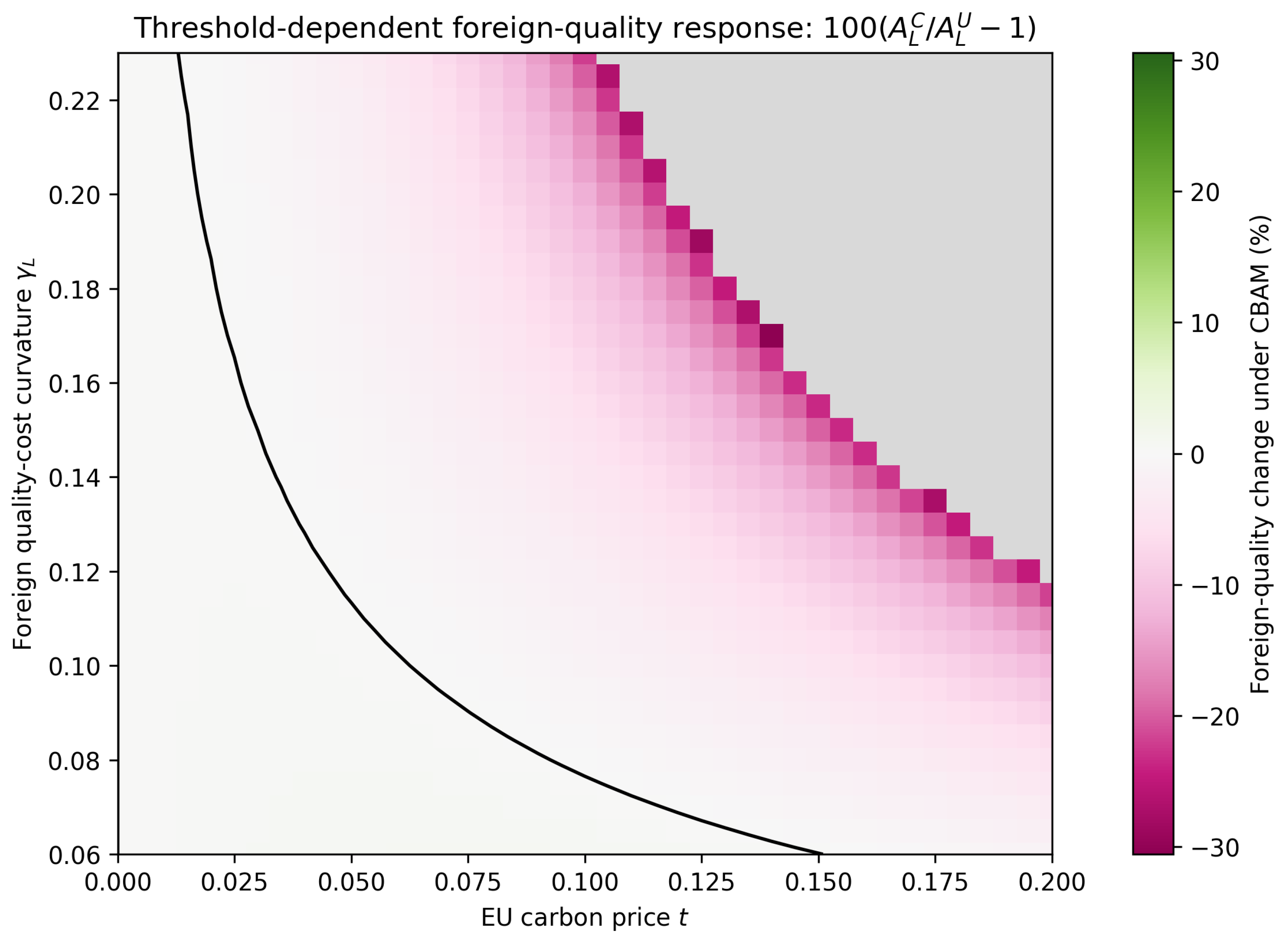
Figure 1 extends the point estimates in Table 2 and Table 3 by mapping the percentage change in foreign environmental quality over the complete primary grid. This is the foreign-quality backfire-region figure: it evaluates the sign of $\Delta A_L$ and should not be interpreted as a figure of aggregate-emissions backfire.

As shown in Figure 1, the black zero contour separates the upgrading region, where $\Delta A_L>0$, from the quality-backfire region, where $\Delta A_L<0$. Consistent with Table 3, the contour slopes downward: as ${\gamma }_L$ increases, a smaller carbon price is sufficient to reverse the foreign firm’s equilibrium quality response. The figure also shows that the magnitude of the decline generally becomes larger as one moves farther into the high-t, high-${\gamma }_L$ part of the feasible region. Grey cells are excluded because at least one maintained interior-equilibrium, positive-emissions, or regularity condition fails there.

The economic mechanism is also threshold-dependent. Close to free trade, the direct saving in the foreign firm’s carbon payment raises its marginal return to environmental quality. At higher effective carbon charges, however, the foreign firm’s price-cost margin and demand contract. Quality investment is then monetized over a smaller market. When ${\gamma }_L$ is sufficiently large, this market-contraction effect exceeds the direct carbon-cost saving and the equilibrium quality response reverses. We, therefore, avoid referring to “low” and “moderate” carbon prices without a defined boundary; throughout this section, those regions are defined by $t<t^{*}\left({\gamma }_L\right)$ and $t>t^{*}\left({\gamma }_L\right)$, respectively.

4.3. Baseline-Emissions Asymmetry

Table 4. Sensitivity to foreign baseline emissions intensity at $t=0.10$.

${\mathit{a}}_{\mathit{L}}$	${\mathit{A}}_{\mathit{L}}^{\mathit{U}}$	${\mathit{A}}_{\mathit{L}}^{\mathit{C}}$	$100({\mathit{A}}_{\mathit{L}}^{\mathit{C}}/{\mathit{A}}_{\mathit{L}}^{\mathit{U}}-1)$
0.50	0.556	0.549	$-1.3\%$
0.70	0.556	0.529	$-4.8\%$
0.90	0.556	0.495	$-10.9\%$
1.10	0.556	0.411	$-26.1\%$

is a separate sensitivity analysis rather than part of the symmetric baseline specification. It changes $a_L$ while holding $a_H=0.50$, so firms differ in both quality-cost curvature and baseline emissions intensity. Accordingly, the larger quality decline in this table cannot be attributed solely to ${\gamma }_L>{\gamma }_H$. It shows that the market-contraction mechanism becomes stronger when the foreign product enters CBAM with a larger baseline carbon burden.

The baseline specification, therefore, isolates the quality-cost asymmetry ${\gamma }_L>{\gamma }_H$. The asymmetric-emissions exercise in Table 4 deliberately relaxes this restriction by allowing the foreign firm also to have a higher baseline emissions intensity.

4.4. Four Numerical Margins for Aggregate-Emissions Backfire

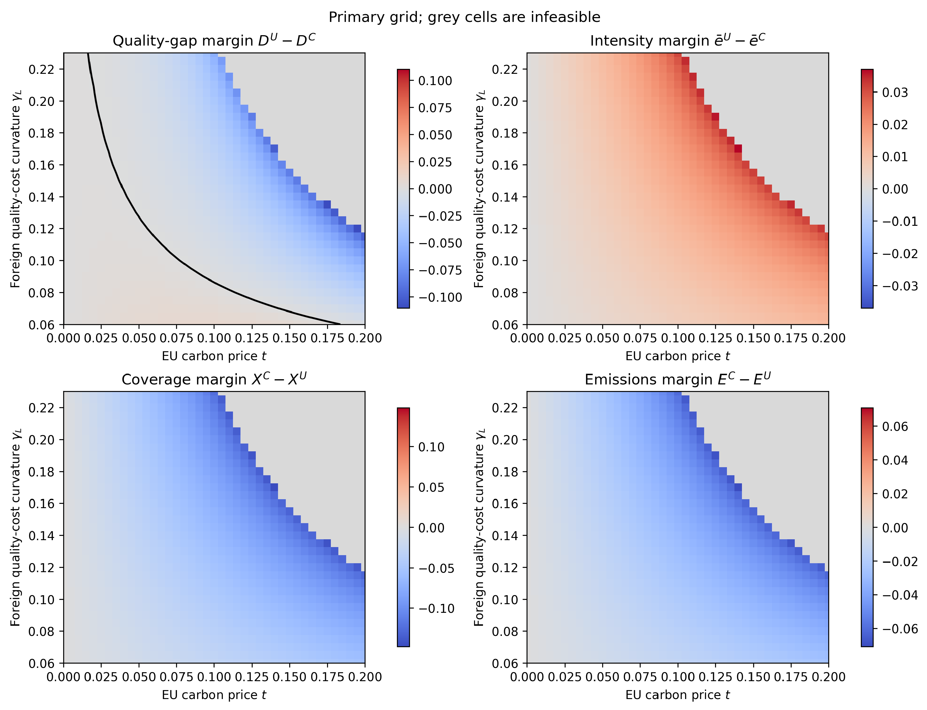
For each feasible grid point, we compute

$$D^U-D^C,{\overline{e}}^U-{\overline{e}}^C,X^C-X^U,E^C-E^U.$$

All four must be positive for the differentiation-collapse mechanism in Corollary 1. Figure 2 displays these four margins over the primary grid used in the foreign-quality analysis. Unlike Figure 1, this figure does not identify the foreign-quality backfire region. Instead, it tests whether the four separate conditions required for aggregate-emissions backfire occur simultaneously.

Figure 2 shows that the average-intensity margin is positive throughout the feasible region, indicating that CBAM lowers average emissions intensity. However, the market-coverage margin $X^C-X^U$ is non-positive at every feasible point, and the aggregate-emissions margin is also non-positive throughout the feasible region. The quality-gap margin changes sign along its black contour, but its positive region never overlaps with positive market-expansion and aggregate-emissions margins. Thus, no feasible point in the primary grid satisfies all four conditions, and no cell has $E^C-E^U>0$ jointly with the other required margins.

The numerical exercise, therefore, supports a scale-contraction interpretation within this specified domain: CBAM reduces total emissions because it contracts market coverage. It does not establish that aggregate-emissions backfire is impossible outside the reported domain or under alternative demand and cost structures.

4.5. Robustness to Production Costs and Incomplete Border Adjustment

We next relax two baseline normalizations. First, for the production-cost robustness checks, marginal cost is

$$m_i=c_i+{\rho }_i(a_i-b{A}_i).$$

The values $c_i\in \{0.02,0.04\}$ represent small positive costs in the normalized price unit. They are of the same order as the equilibrium carbon-cost components at $t=0.10$ and are, therefore, large enough to affect incentives without violating the maintained interior-market conditions.

Second, let $t_F$ denote a carbon price already paid by the foreign firm, $\lambda \in [0,1]$ the share of imports covered by the border adjustment, and $\chi \in [0,1]$ the share of the foreign carbon payment credited by the EU. We write the foreign firm’s effective carbon charges as

$${\rho }_L^U=t_F,{\rho }_L^C=t_F+\lambda \max \{0,t_E-\chi t_F\}.$$

(49)

Baseline full-CBAM case is $t_F=0$, $\lambda =1$, and $\chi =1$. Equation (49) also permits partial product coverage and incomplete recognition of a foreign carbon payment.

Positive common or asymmetric production costs do not eliminate quality backfire in these checks; instead, the foreign-quality reduction ranges from $4.05$ to $8.64$ percent. The result also survives the three specifications that introduce a foreign carbon price, although its magnitude depends on coverage and crediting. It does not survive every incomplete-CBAM design: with 50 percent coverage and no foreign carbon price, foreign quality increases by $0.21$ percent. This finding reinforces the threshold interpretation. Quality backfire is not a universal consequence of CBAM; it arises when the effective foreign carbon charge is large enough, relative to the foreign firm’s quality technology and market position, to make the contraction in the return to quality dominate the direct tax-saving incentive. Aggregate-emissions backfire is absent in every robustness scenario in

Table 5. Robustness at $t_E=0.10$, $a_H=a_L=0.50$, and ${\gamma }_L=0.10$.

Scenario	${\mathit{\rho }}_{\mathit{L}}^{\mathit{U}}$	${\mathit{\rho }}_{\mathit{L}}^{\mathit{C}}$	$\%\mathbf{\Delta }{\mathit{A}}_{\mathit{L}}$	${\mathit{E}}^{\mathit{C}}-{\mathit{E}}^{\mathit{U}}$
Zero production costs; full CBAM	0.0000	0.1000	$-1.25$	$-0.0214$
$c_H=c_L=0.02$	0.0000	0.1000	$-4.21$	$-0.0224$
$c_H=0.02,c_L=0.04$	0.0000	0.1000	$-8.64$	$-0.0252$
$c_H=0.04,c_L=0.02$	0.0000	0.1000	$-4.05$	$-0.0222$
$\lambda =0.50,t_F=0$	0.0000	0.0500	$+0.21$	$-0.0106$
$t_F=0.025, \lambda =1, \chi =1$	0.0250	0.1000	$-1.55$	$-0.0162$
$t_F=0.025, \lambda =0.50, \chi =1$	0.0250	0.0625	$-0.29$	$-0.0080$
$t_F=0.025, \lambda =1, \chi =0.50$	0.0250	0.1125	$-2.21$	$-0.0190$

; all reported emissions differences remain negative.

4.6. Numerical Conclusions

The numerical analysis establishes a conditional, finite-price mechanism. Sufficiently close to the free-trade limit, Remark 2 establishes analytically that the foreign firm’s equilibrium quality is higher under CBAM than under unilateral pricing. Beyond a threshold $t^{*}\left({\gamma }_L\right)$, the equilibrium market-contraction effect may dominate and lower $A_L$ relative to unilateral pricing. The threshold decreases as foreign quality adjustment becomes more costly and the effect becomes stronger when the foreign product has higher baseline emissions. The result persists under the reported positive and asymmetric production-cost checks and under several foreign-carbon-price and crediting specifications, but it is not present over the entire parameter grid or under every incomplete-CBAM design. By contrast, the proposed aggregate-emissions backfire remains an analytical possibility that is not realized in the baseline grid or the reported robustness exercises.

5. Welfare Implications

The analysis so far has evaluated CBAM using two environmental outcomes: the foreign firm’s environmental-quality choice and aggregate emissions. Neither, however, is by itself a welfare criterion. The market-contraction mechanism underlying quality backfire also affects consumer surplus, firms’ profits, and carbon revenue. We, therefore, complement the preceding analysis with an ex post welfare comparison of unilateral pricing and full CBAM.

For this exercise, we return to the baseline policy regimes of Section 3.4, with zero production costs and no foreign carbon price. Thus, under unilateral pricing ${\rho }_H=t$ and ${\rho }_L=0$, while under full CBAM ${\rho }_H={\rho }_L=t$. The extensions involving a foreign carbon price, partial coverage, and incomplete crediting in Section 4.5 are not included in the welfare accounting below.

5.1. Welfare Accounting and the Critical Social Cost of Carbon

For regime $r\in \{U,C\}$, equilibrium consumer surplus is

$$C{S}^r={\int }_{{\theta }_0^r}^{{\theta }_1^r}(\theta A_L^r-p_L^r)d\theta +{\int }_{{\theta }_1^r}^1(\theta A_H^r-p_H^r)d\theta .$$

Using $x_L^r={\theta }_1^r-{\theta }_0^r$ and $x_H^r=1-{\theta }_1^r$, this can be written compactly as

$$C{S}^r={\displaystyle \frac{A_L^r}{2}}{\left(x_L^r\right)}^2+A_L^r{x}_L^r{x}_H^r+{\displaystyle \frac{A_H^r}{2}}{\left(x_H^r\right)}^2.$$

(50)

For welfare accounting, we interpret the modeled carbon charge as a tax or auctioned-permit payment accruing to the EU and assume that the resulting revenue is recycled lump-sum, so that carbon payments are transfers rather than resource costs. Under the baseline regimes considered here, EU carbon revenue is, therefore,

$$R_E^U=t{e}_H\left(A_H^U\right)x_H^U,R_E^C=t\left[e_H\left(A_H^C\right)x_H^C+e_L\left(A_L^C\right)x_L^C\right].$$

(51)

Let $\delta \ge 0$ denote the social cost of one unit of emissions, expressed in the same normalized units as prices and profits. EU welfare is

$$W^{EU,r}=C{S}^r+{\mathrm{\Pi }}_H^r+R_E^r-\delta E^r.$$

(52)

This accounting follows the standard partial-equilibrium environmental-policy welfare analysis, in which consumer surplus, producer surplus, policy revenue, and monetized environmental damages enter the welfare objective; see, for example, Bansal and Gangopadhyay (2003) and Elhadj and Tarola (2015). A closely related carbon-tariff formulation is provided by Drake (2018).

We also consider welfare for the modeled EU market when the foreign firm’s profit is included:

$$W^{G,r}=C{S}^r+{\mathrm{\Pi }}_H^r+{\mathrm{\Pi }}_L^r+R_E^r-\delta E^r.$$

(53)

Since ${\mathrm{\Pi }}_i^r$ is the equilibrium payoff defined in Equation (9), it already nets out the firm’s environmental-quality investment cost ${\gamma }_i{\left(A_i^r\right)}^2/2$; no additional quality-cost term is, therefore, required in the welfare expressions.

The distinction is useful because the EU criterion excludes foreign producer surplus, whereas the second measure internalizes the foreign firm’s profit. The latter should be interpreted as a global welfare measure for the market represented in the model, rather than as a complete accounting of world welfare.

For any variable z, define the regime difference

$$\Delta z\equiv z^C-z^U.$$

Let

$$\Delta G^{EU}\equiv \Delta CS+\Delta {\mathrm{\Pi }}_H+\Delta R_E$$

and

$$\Delta G^G\equiv \Delta CS+\Delta {\mathrm{\Pi }}_H+\Delta {\mathrm{\Pi }}_L+\Delta R_E$$

denote the corresponding non-environmental surplus changes. Then

$$\Delta W^k=\Delta G^k-\delta \Delta E,k\in \{EU,G\}.$$

(54)

Proposition 4

(Critical social cost of carbon). Suppose full CBAM reduces total EU-market emissions relative to unilateral pricing, $\Delta E<0$. For either welfare criterion $k\in \{EU,G\}$,

$$\Delta W^k>0⟺\delta >{\delta }^{*k}\equiv {\displaystyle \frac{\Delta G^k}{\Delta E}}.$$

If $\Delta G^k>0$, CBAM strictly raises welfare for every $\delta \ge 0$. If $\Delta G^k=0$, it weakly raises welfare for every $\delta \ge 0$ and strictly raises welfare whenever $\delta >0$. If $\Delta G^k<0$, CBAM raises welfare only when the social cost of carbon exceeds the positive threshold ${\delta }^{*k}$.

Proof. 

From Equation (54), $\Delta W^k>0$ if and only if $\Delta G^k>\delta \Delta E$. Since $\Delta E<0$, division by $\Delta E$ reverses the inequality and yields $\delta >\Delta G^k/\Delta E$. □

Proposition 4 separates the product-market and distributional consequences of CBAM, summarized by $\Delta G^k$, from the welfare benefit of its emissions effect, $-\delta \Delta E$. Section 4.4 shows that $\Delta E<0$ throughout the feasible baseline grid, so the environmental component is positive in the numerical region considered there.

5.2. Numerical Welfare Comparison

Table 6. Welfare effects of full CBAM relative to unilateral pricing.

${\mathit{\gamma }}_{\mathit{L}}$	$\%\mathbf{\Delta }{\mathit{A}}_{\mathit{L}}$	$\mathbf{\Delta }\mathit{CS}$	$\mathbf{\Delta }{\mathbf{\Pi }}_{\mathit{H}}$	$\mathbf{\Delta }{\mathbf{\Pi }}_{\mathit{L}}$	$\mathbf{\Delta }{\mathit{R}}_{\mathit{E}}$	$\mathbf{\Delta }\mathit{E}$	${\mathit{\delta }}^{*\mathit{EU}}$	${\mathit{\delta }}^{*\mathit{G}}$
0.06	$+0.7$	$-0.0110$	$+0.0115$	$-0.0108$	$+0.0107$	$-0.0133$	$-0.844$	$-0.029$
0.08	$-0.2$	$-0.0127$	$+0.0126$	$-0.0108$	$+0.0104$	$-0.0173$	$-0.598$	$+0.030$
0.10	$-1.3$	$-0.0140$	$+0.0134$	$-0.0108$	$+0.0101$	$-0.0214$	$-0.445$	$+0.058$
0.13	$-3.4$	$-0.0157$	$+0.0146$	$-0.0106$	$+0.0095$	$-0.0281$	$-0.298$	$+0.081$
0.17	$-7.8$	$-0.0180$	$+0.0161$	$-0.0103$	$+0.0085$	$-0.0380$	$-0.174$	$+0.098$
0.22	$-18.0$	$-0.0225$	$+0.0190$	$-0.0098$	$+0.0069$	$-0.0549$	$-0.060$	$+0.118$

Notes: Calibration: $a_H=a_L=0.50$, $b=0.05$, ${\gamma }_H=0.05$, and $t=0.10$. All welfare components are reported in normalized model units. The critical values ${\delta }^{*EU}$ and ${\delta }^{*G}$ are calculated from the unrounded equilibrium values, so they need not equal ratios constructed from the rounded entries shown in the table.

reports the welfare decomposition at $t=0.10$ over the same values of ${\gamma }_L$ used in Table 2. All entries are differences between full CBAM and unilateral pricing.

Three features are worth emphasizing. First, CBAM lowers consumer surplus throughout the reported range, consistent with the market contraction documented in Section 4.4. At the same time, the home firm’s profit and EU carbon revenue increase. In the reported comparisons, these two gains more than offset the loss of consumer surplus, so that $\Delta G^{EU}>0$ and ${\delta }^{*EU}<0$ throughout the table. Thus, at these parameter values, full CBAM raises EU welfare even when emissions are assigned no social cost; the reduction in emissions further reinforces this welfare gain. This pattern reflects both the environmental consequences of CBAM and a redistribution of surplus toward the regulating jurisdiction.

Second, the global-market welfare comparison is more demanding because the foreign firm’s profit loss is also counted. At ${\gamma }_L=0.06$, $\Delta G^G>0$, whereas from ${\gamma }_L=0.08$ onward the non-environmental global-surplus effect becomes negative. CBAM then raises global-market welfare only when the value assigned to its emissions reduction exceeds the positive threshold ${\delta }^{*G}$. The required threshold rises as the foreign firm’s quality-adjustment disadvantage becomes larger.

Third, the welfare and technology criteria are distinct. In particular, quality backfire, $A_L^C<A_L^U$, can coexist with higher EU welfare and can also coexist with higher global-market welfare when the environmental benefit is sufficiently large. Conversely, an improvement in the foreign firm’s environmental quality does not by itself establish that CBAM is welfare improving. The technology response, aggregate-emissions response, and welfare ranking should, therefore, be evaluated separately.

These welfare calculations remain deliberately partial-equilibrium and normalized. They cover consumers and production associated with the modeled EU market, but not foreign consumer surplus, emissions associated with sales outside that market, or foreign-government revenue under the extended policy specifications of Section 4.5. Moreover, $\delta$ is expressed in normalized model units and should not be interpreted directly as euros per tonne without a sector-specific mapping. The exercise is, therefore, intended to clarify the welfare mechanisms and their thresholds rather than to provide an empirical estimate of the welfare effects of the EU CBAM.

6. Discussion and Conclusions

6.1. Discussion

The results complement the border-carbon-adjustment literature by identifying a firm-level adjustment margin that is absent when production technology is treated as fixed. Existing work emphasizes changes in trade, output, leakage, and aggregate emissions, while more recent models allow firms to adjust abatement endogenously. Consistent with the former literature, our numerical analysis finds that CBAM reduces aggregate emissions over the reported parameter region mainly through market contraction. The additional result here is that this aggregate improvement can coexist with a deterioration in the foreign firm’s environmental technology.

The mechanism arises because environmental performance is also a product-positioning decision. Relative to endogenous-abatement models such as Ambec et al. (2024) and Fikru et al. (2025), environmental quality in our model is a vertically differentiating attribute chosen in anticipation of Bertrand price competition. Extending the carbon charge to imports, therefore, has two opposing effects: it creates a direct incentive for the foreign firm to improve quality, but also changes the margin and market share over which quality investment earns a return. The local analysis shows that the first effect dominates sufficiently close to free trade, whereas Section 4 shows that the ordering can reverse once the carbon price exceeds a parameter-dependent threshold. Thus, the contribution is not simply that firms respond endogenously to carbon policy, but that the environmental and competitive positioning decisions are jointly determined and can generate a finite-price reversal of the intended technology response.

These results also qualify their own policy interpretation. Equalizing carbon prices at the border need not be sufficient to equalize firms’ incentives to adopt cleaner technology, because the policy also reshapes product-market returns. At the same time, the welfare analysis in Section 5 shows that quality backfire should not itself be interpreted as welfare backfire: consumer surplus, producer rents, carbon revenue, and aggregate emissions may move in different directions. The conclusions remain conditional on the model’s vertically differentiated duopoly, uncovered market, and exogenous policy regime. The robustness exercises show that the quality-backfire mechanism survives several positive-cost and incomplete-CBAM specifications, but not every such specification, and its prevalence under richer market structures or endogenous government policy remains an open question.

6.2. Conclusions

Bringing the results together, CBAM’s firm-level, aggregate-emissions, and welfare effects are closely connected through its impact on the foreign exporter’s margin and market share. The contraction of these product-market returns can overturn the direct incentive to improve environmental quality, leaving the foreign firm dirtier than under unilateral pricing once the carbon price exceeds a parameter-dependent threshold (Section 4). The welfare consequences are distinct but related: in the reported numerical comparisons, CBAM raises EU welfare even at a zero social cost of carbon, whereas the global-market welfare gain may require a sufficiently high valuation of the resulting emissions reduction.

The paper’s central result is, therefore, a threshold-dependent quality reversal. Our local implicit-function analysis establishes that sufficiently close to free trade the foreign firm chooses higher environmental quality under CBAM than under unilateral pricing. As the carbon charge increases, however, the associated contraction in the foreign firm’s margin and market share can reduce the return to quality investment enough to reverse this ordering. The numerical analysis identifies the corresponding parameter-dependent thresholds and shows that the reversal occurs over a substantial part of the admissible parameter region and persists under the reported production-cost and several incomplete-CBAM robustness checks.

A distinct result concerns aggregate emissions. By narrowing the quality gap, CBAM can, in principle, intensify price competition and expand the market enough to raise total emissions even as average intensity improves. We derive the exact threshold condition under which this scale effect would dominate the technique effect by adapting the Grossman–Krueger and Copeland–Taylor decomposition to firm-level quality choice. However, in our numerical calibration, this channel is not the operative force: CBAM reduces total emissions mainly through market contraction rather than through differentiation collapse.

The welfare analysis reinforces the distinction between environmental and welfare performance. In the reported numerical comparisons, CBAM’s gains in home producer profit and EU carbon revenue more than offset the loss in consumer surplus, while global-market welfare may require a sufficiently high valuation of the emissions reduction once the foreign firm’s profit loss is included. Quality backfire, therefore, does not by itself imply welfare backfire.

The model deliberately isolates these mechanisms in a stylized duopoly with an exogenous carbon-pricing regime. Natural extensions include richer market structures and an endogenous policy game in which the EU border adjustment interacts with the exporting country’s carbon policy. More broadly, in light of the EU CBAM’s definitive phase beginning in January 2026, the analysis suggests that the effectiveness of border carbon adjustment depends not only on equalizing carbon-price exposure, but also on how the policy reshapes firms’ incentives to invest in cleaner technology through its effects on product-market returns in the carbon-intensive industries they are meant to regulate.