Article

Provision of Public Goods via Unilateral but Mutually Conditional Commitments—Mechanism, Equilibria, and Learning

Potsdam Institute for Climate Impact Research, P.O. Box 60 12 03, 14412 Potsdam, Germany
Games 2025, 16(6), 58; https://doi.org/10.3390/g16060058
Submission received: 30 September 2025 / Revised: 30 October 2025 / Accepted: 3 November 2025 / Published: 5 November 2025
(This article belongs to the Section Non-Cooperative Game Theory)

Abstract

We propose a one-shot, non-cooperative mechanism that implements the core in a large class of public goods games. Players simultaneously choose conditional commitment functions, which are binding unilateral commitments that condition a player’s contribution on the contributions of others. We prove that the set of strong Nash equilibrium outcomes of this mechanism coincides exactly with the core of the underlying cooperative game. We further show that these core outcomes can be found via simple individual learning dynamics.
JEL Classification:
H41; D47; F53; C72; C71; D43

1. Introduction

Public goods are systematically underprovided due to free-riding incentives. While binding agreements and repeated games offer theoretical solutions, many real-world contexts lack strong enforcement mechanisms or sufficient repetition. This paper studies a third approach: unilateral but mutually conditional commitments.
Our contribution. We introduce a one-shot, non-cooperative mechanism where players simultaneously choose conditional commitment functions (CCFs) that bind their contributions to the contributions of others. Our main theoretical result establishes an exact equivalence: the set of strong Nash equilibrium outcomes of this mechanism coincides with the core of the underlying cooperative game. As a second contribution, we prove that simple individual learning dynamics converge to these core outcomes, demonstrating practical implementability.
This mechanism formalizes emerging real-world practices. The US National Popular Vote Interstate Compact (Bennett, 2001; Muller, 2007) exemplifies such conditional commitments. In it, federal states unilaterally commit to electoral reforms conditional on sufficient other states making similar commitments. Similarly, conditional Intended Nationally Determined Contributions under the Paris Agreement (Pauw et al., 2020) allow countries to pledge emission reductions contingent on others’ actions.
Relationship to the existing literature. Our work contributes to the core implementation literature by providing what appears to be the first one-shot mechanism implementing the core in public goods games—a contribution to the Nash program of justifying cooperative solution concepts through non-cooperative mechanisms. We extend the conditional commitment literature beyond the setting of Reischmann and Oechssler (2018) and Oechssler et al. (2022) to continuous action spaces with generic utility functions. While our mechanism shares mathematical similarities with supply function equilibria (Delgado & Moreno, 2004; Klemperer & Meyer, 1989), it achieves efficiency rather than merely replicating Nash outcomes. Also, although CCFs are similar to best-response functions in (quasi-)supermodular games (Milgrom & Shannon, 1994) in that they are non-decreasing, our mechanism is not a quasi-supermodular game in itself, as the best-response CCF to an opponent’s CCF is not necessarily a non-decreasing function of that CCF (see Appendix E for a counterexample).
The mechanism. Each player i submits a conditional commitment function, c i : A i A i , mapping others’ action profiles to their own commitment level. The mechanism selects the largest mutually feasible action profile ( c ) = sup { a : a i c i ( a i ) for all i } . Unlike best-response functions that typically yield low contributions in public goods games, CCFs enable commitments to high contribution levels.
Our theoretical analysis covers a general class of costly positive externality problems where players prefer to contribute less themselves while benefiting from others’ contributions. We prove that strong Nash equilibria exist if and only if the core is nonempty and establish core nonemptiness for important special cases including separable utility functions and Cournot oligopolies.
The learning results show that when players iteratively update CCFs by choosing favorite points in others’ feasible sets and responding with indifference curve commitments, the process converges to core outcomes. This provides a constructive path to efficiency without central coordination.
Our mechanism also generalizes existing approaches: the approach of Gerber and Wichardt (2009) can be viewed as one that restricts players to a single conditional commitment (contribute optimally if all others do), while matching mechanisms (Buchholz et al., 2011) prescribe, rather than endogenize, the dependence of contributions on others’ actions.
This paper proceeds as follows: Section 2 defines the CCF mechanism for single public goods. Section 3 establishes the core equivalence result and proves core nonemptiness. Section 4 analyzes learning dynamics with applications to climate policy. Section 5 concludes the paper.

2. The Conditional Commitment Function Mechanism

In this section, we describe the CCF mechanism for a case where each player contributes only to one public good, whether the same or different ones, saving the technically more involved treatment of the case of more than one action dimension per player for the Appendix A, Appendix B and Appendix C.
We assume the following: All N > 1 players, i, can supply any non-negative amount q i 0 of some public good (which might or might not be the same good for all players). From everyone’s contributions, i derives utility v i ( q ) , where q = ( q 1 , , q N ) is the players’ joint supply profile. For convenience, we sometimes also write ( q i , q i ) instead of q, where q i = ( q 1 , , q i 1 , q i + 1 , , q N ) is the other players’ supply profile. Each i has an optimal amount q i 0 that maximizes v i ( q i , q i ) for all q i . In the domain where q i q i 0 and all q j q j 0 , j i , the function v i is weakly increasing in each q j , j i and weakly decreasing in q i .
If the players were to play the one-shot game of choosing q i directly and simultaneously, it would be a strictly dominant strategy to choose q i = q i 0 . This unique strategic equilibrium would lead to individual and joint utilities of u i 0 = v i ( q 0 ) and U 0 = i u i 0 . Let us call this the unconditional equilibrium.
As is well known, the socially optimal contributions and resulting joint utility are typically much larger than this. Consider the simple symmetric case with linear benefits and linear marginal costs, where v i ( q ) = j = 1 N q j q i 2 / 2 . In that case, q i 0 = 1 and U 0 = N ( N 1 / 2 ) . In contrast, the social optimum would have q i = N and total utility U = N 3 / 2 . The quotient between U and U 0 , N 2 / ( 2 N 1 ) , is then basically proportional to the number of players N.
The classical challenge in this social dilemma is to find a mechanism that incentivizes players to supply more than the unconditional equilibrium. To focus on this, and using a little more general terminology, we introduce the notation a i = q i q i 0 and call a i the action of player i. Here, a i is represented by a single real number, while in the more general case addressed in the Appendix A, Appendix B and Appendix C, it can be an element of any partially ordered set. When dealing with utilities, we will also use the utility functions in terms of actions, u i ( a ) = v i ( q 0 + a ) . Since the socially optimal contributions q i are above the equilibrium ones q i 0 , we restrict our focus to non-negative actions a i [ 0 , ) , so that our above assumptions imply that u i ( a ) is weakly decreasing in a i and weakly increasing in a i .
Now, the following CCF mechanism allows players to sustain the socially optimal levels q in equilibrium. Instead of choosing a i directly, in the CCF mechanism, each player simultaneously submits a conditional commitment function (CCF), c i : [ 0 , ) N 1 [ 0 , ) , that maps each possible action profile a i of the others to a “limit” c i ( a i ) for the player. Only CCFs which are weakly increasing in each argument a j are allowed. The interpretation is that by submitting c i , player i commits to accept the liability to realize any level a i c i ( a i ) if a i are the liabilities of the others. From the profile c = ( c 1 , , c N ) of submitted CCFs, the CCF mechanism determines the set of feasible action profiles:
F ( c ) = { a : a i c i ( a i ) for all i } .
It then selects its largest element, ( c ) = sup F ( c ) , as the liabilities the players have to fulfill. In Lemma A2 in Appendix B.1, we show that F ( c ) is nonempty and, indeed, that it has a largest element. In our one-dimensional case, it is simply given by
( c ) i = max { a i : a F ( c ) } .
So, in game-theoretic terms, the CCF mechanism is the one-shot simultaneous-move game form in which player i’s strategy (or “message”) space is the set of possible CCFs c i , and the outcome is the action profile ( c ) . In terms of the public good, this means that each player then supplies an amount of q i 0 + ( c ) i .1
Depending on the application context, the mechanism can be implemented in different ways. In a domestic context, a regulator might set up a central institution similar to a stock exchange that accepts CCF submissions rather than bids and offers and then announces resulting liabilities. In an international context, countries might pass domestic legislation that commits them to realizing their part of ( c ) based on a CCF they specify in that bill and the CCFs that other countries passing similar legislation state in their respective bills—somewhat similar to how the US National Popular Vote Interstate Compact works.
Note that players can choose any kind of function c i as their CCF as long as it is weakly increasing. Figure 1a shows a two-player example with continuous CCFs, in which case the outcome ( c ) is simply the uppermost intersection of c 1 and c 2 . Two special types of CCFs turn out to be particularly interesting: simple step functions and indifference curves.
Step functions correspond to specific offers. A player could choose some combination of “target levels”, q t , translate it into target actions, a t = q t q 0 , and submit as her CCF the simple step function with
c i ( a i ) = a i t if a j a j t for all j i , c i ( a i ) = 0 otherwise .
She would thus make sure that she will contribute her target, q i t , only if all others contribute at least their targets, q j t , and she will otherwise contribute the unconditional equilibrium value. We will call this type of CCF a canonical CCF through a t . Examples of canonical CCFs and resulting outcomes are seen in Figure 1b.
While it will turn out that canonical CCFs already suffice to construct strong equilibria leading to efficient outcomes, the learning rules that find these equilibria will also require a second special type of CCF that correspond to more general offers. If a player’s utility function, u i ( a ) , is continuous in a, she could choose a “target utility”, u i t , and submit, as her CCF, the largest function that guarantees this utility level whenever possible:
c i ( a i ) = max { a i 0 : u i ( a i , a i ) u i t } if u i ( 0 , a i ) u i t ,
c i ( a i ) = 0 otherwise .
This way, she would act as a “satisficer” who offers to supply any amount strictly above the unconditional equilibrium if she gets at least her target utility. If u i t is given by i’s utility in some reference profile, a t , we call this type of CCF an indifference curve CCF through a t . Examples of indifference curve CCFs and resulting outcomes can be seen in Figure 1c.

3. Correspondence Between Strong Equilibria and Core Action Profiles

Let us now study the strategic implications of the CCF mechanism. When considering only stability against single-player deviations, it turns out that there are very many equilibria, both efficient and inefficient ones:
Theorem 1.
For the class of public goods problems considered in the main text, an action profile a is the outcome of some pure-strategy Nash equilibrium of the CCF mechanism if and only if u i ( a ) u i 0 for all players i. In particular, every Pareto-efficient combination of public good supplies, q, can be sustained in pure-strategy Nash equilibrium, and this requires canonical CCFs only.
This nonsurprising fact follows directly from the first part of Theorem A1 in Appendix B.2; see the formal proof there. The main reason for this result is the following. Assume all players weakly prefer a to the zero action profile and submit their canonical CCF through a. Then, any deviation by a single player i that changes the outcome either makes i supply more or makes all others’ actions go down to zero (i.e., to the unconditional equilibrium levels), but neither of these two things does player i prefer to a.
A more thorough analysis takes into account that several players may plan deviations together. For studying stability against such joint deviations, the proper game-theoretic solution concepts are coalition-proof Nash equilibrium (Bernheim et al., 1987) and strong Nash equilibrium (Aumann, 1959). We only discuss strong equilibrium here, as we show in Theorem A1 in Appendix B.2 that, in our context, both concepts are essentially equivalent. For a pure strategy equilibrium to be strong, no group (“coalition”) of players must have a joint deviation producing an outcome that all members of that group prefer (for subtleties regarding weak and strong preferences; see Appendix A).
To see that this makes a difference, note that any outcome a of a strong equilibrium must necessarily be Pareto-efficient. If not, there would be an alternative action profile a that all players would prefer to a, and by changing everyone’s CCF to their canonical CCF through a , they could jointly produce that preferred outcome. However, characterising the whole set of action profiles that may result from some strong equilibrium in the CCF mechanism is not that trivial. We will see that it coincides with a certain version of the ‘core’ of the underlying public goods problem.
The basic idea of a core action profile is that no group of players can “on their own” produce a different outcome they all prefer by switching to a different combination of actions. (Note that while a strong equilibrium of the CCF mechanism is a profile of CCFs, a core action profile is a much simpler object: a profile of actions in the underlying public goods problem.) Formally, given utility functions u i , we call an action profile a a core outcome if and only if there is no group G of players and action profile a so that a j = 0 for all players j outside G and so that u i ( a ) > u i ( a ) for all i G .2
Theorem 2.
For the class of public goods problems considered in the main text, an action profile a is the outcome of some strong Nash equilibrium of the CCF mechanism if and only if it is a core action profile. To sustain a core action profile in strong equilibrium, it suffices to use canonical CCFs. If all utility functions are continuous, it also suffices to use indifference curve CCFs. In particular, every strong equilibrium outcome is Pareto-efficient.
Again, this follows from Theorem A1 in Appendix B.2.3 The main reason for this result is that when all players submit their canonical or indifference curve CCF through a core action vector a, then each deviation by some group either makes every group member supply no less than in a, or makes all non-group members switch to action zero; but neither of these consequences do all group members prefer to a.
Note that the theorem does not imply that the core is nonempty or that there is any strong Nash equilibrium in the first place. In fact, it is well known that cores might be empty. Especially for public goods problems, however, Chander and Tulkens (1997) have shown that the core of public goods problems is often nonempty. In particular, one can easily see, with the help of the Bondareva-Shapley theorem, that the core is nonempty if utility is separable into costs and quasi-linear benefits of the form u i ( a ) = f i ( j α i j a j ) g i ( a i ) , where f i are weakly increasing and weakly convex benefit functions, α i j are nonnegative coefficients, and g i are arbitrary cost functions (see Lemma A1 in Appendix A.4 for a proof).
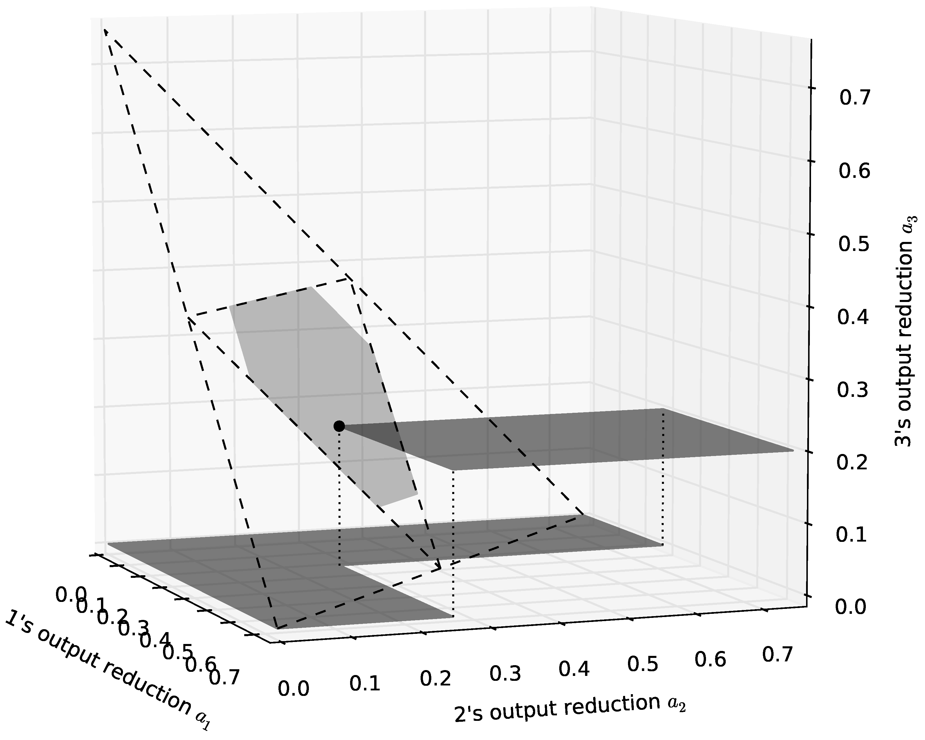
Another example where the core is nonempty is when utility has the quadratic form u i ( a ) = ( α a i ) 3 j ( α a j ) with α = 3 / ( N + 1 ) , where actions are constrained to 0 a i α . These utility functions arise when players are firms in a Cournot oligopoly with outputs y i , uniform marginal production costs of unity, and demand function Y ( P ) = 4 P , where P is the price. In that case, firm i’s output reduction with respect to the Cournot equilibrium output, which is y 0 = 3 / ( N + 1 ) = α , is the quantity a i = y 0 y i 0 , which can be interpreted as that firm’s contribution to a “public” good among the firms (actually a club good). For N = 3 , Figure 2 shows the core of this problem as a light grey hexagon and depicts a canonical CCF for player 3 through some core point (large dot) as a dark grey step function. Together with the canonical CCFs of the other two players through that point, it forms a strong equilibrium that sustains that efficient outcome.

4. Finding Strong Equilibria via Simple Learning Rules

A strong equilibrium would not be worth much if players have no way to find it and converge to it. In this section, we will see how with the CCF mechanism, players can use a simple learning rule to achieve this, either asymptotically or even in only a small finite number of steps. We assume all utility functions u i are continuous in this section.
General learning rule. The learning rules we consider here are of the following simple type. Players start with all-zero CCFs, c i ( a i ) 0 , and then iteratively and repeatedly adjust their CCFs independently and without a need to communicate or negotiate other than indirectly by adjusting their individual CCFs. In each iteration, some player, i, (e.g., a randomly drawn one) identifies a favourite point (action profile) in the feasible set defined by the other players’ current CCFs. In other words, she picks some a for which u i ( a ) is largest among all a that fulfill the conditions a j c j ( a j ) for all j i . Let us call the chosen point o, let c i o be i’s canonical CCF through o, and let c ˜ i o be i’s indifference curve CCF through o. She then replaces her current CCF by a new function c i , which is between c i o and c ˜ i o . In other words, she puts c i o ( a i ) c i ( a i ) c ˜ i o ( a i ) for all a i .
This can be interpreted as players treating others’ CCFs as a set of offers to which they adjust by making a set of counteroffers that lead to mutual improvement. By offering, at most, their indifference curve through their current favourite item on the others’ “offer menu”, they make sure the future outcomes can only be better than that point if they require the player to contribute positively.
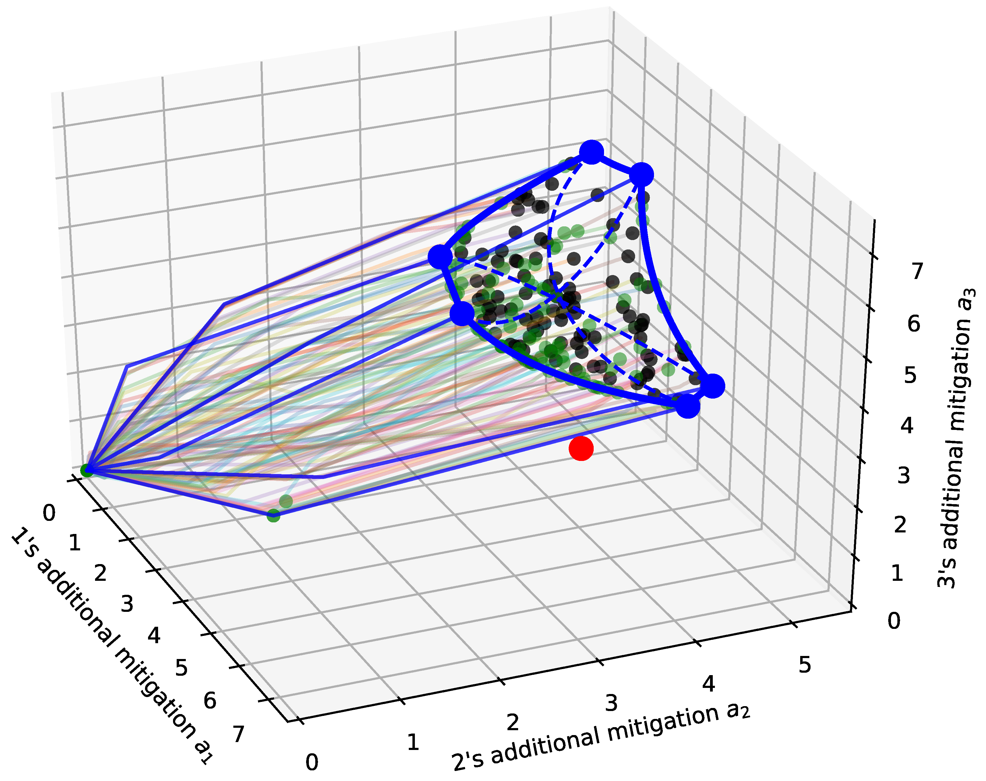
For example, the updates could simply use convex combinations: pick a number 0 λ 1 and put c i = ( 1 λ ) c i o + λ c ˜ i o . Figure 3 shows the dynamics generated by this rule in a public goods problem typical for the literature on international environmental agreements (Barrett, 1994):
Example. Three emitting countries can reduce their greenhouse gas emissions by an amount q i with respect to some business-as-usual scenario, leading to total mitigation of Q = q 1 + q 2 + q 3 and welfare levels v i ( q ) = β i Q q i 2 / 2 γ i , where β = ( 1 , 1.5 , 2 ) are climate damage factors, and γ = ( 2 , 1 , 1.5 ) are mitigation cost coefficients. In this case, the individually rational mitigation levels are q i 0 = β i γ i , the ‘action’ in our terminology is additional mitigation, a i = q i β i γ i , and utility functions in terms of actions are u i ( a ) = β i ( a 1 + a 2 + a 3 + 6.5 ) ( a i + β i γ i ) 2 / 2 γ i . The core of this problem is a curved surface whose boundary is shown in Figure 3 by thick blue lines. While all core points are Pareto-efficient, note that, here, the action profile that maximizes total welfare (the red dot) is not in the core, so it cannot be sustained in strong equilibrium, but only in simple Nash equilibrium via the CCF mechanism. Now, assume all three countries pass domestic laws containing some CCF and the commitment to realize the CCF mechanism outcome, and every year some country replaces their CCF as described above, using a random convex combination. Then, the resulting mitigation liabilities would evolve from zero to some core point, similar to the light colored lines in Figure 3, which are 100 different numerical simulations of this probabilistic learning process, each 30 years long. Only very few simulations have not well converged to the core within this time. These numerical results also suggest that the limit points cover the whole core.
While these numerical results are encouraging, it would be nice to have theoretical reason to expect such convergence. Our first result concerns the special case where players act modestly and simply use their indifference curve through o as their new CCF.
Theorem 3.
Assume players start from all-zero CCFs, and then in some random order, each player once replaces their CCF by their indifference curve through a favourite point on the others’ current CCFs. Then, after one such round of updates, the outcome of the CCF mechanism is in the core.
This is a special case of Theorem A2 in Appendix C.1.4 The thin blue lines and blue dots in Figure 3 show the results of this rule. It turns out that, in this example, the six different orders in which the players may update exactly lead to the six corners of the core.5 In Theorem A3 in Appendix C.1, we also give sufficient conditions for ending up in the core after only one round of updates, when players start from nonzero, rather than all-zero, CCFs and apply the same learning rule.
While the modest behaviour studied above leads quickly into the core, it appears not utterly realistic, since a player early in the line will later realize she could have gotten more than provided by the optimal feasible profile at the time she made her choice if she had offered to the later players less than what was given by her indifference curve. Our last result indicates that for other special cases of the general learning rule, it might be possible to prove eventual convergence to the core as well.
Theorem 4.
Assume players start with all-zero CCFs, and in each time step, a random player replaces her CCF by a random convex combination of her canonical and indifference curve CCFs through a favourite point on the others’ current CCFs. Then, if the resulting sequence of outcomes of the CCF mechanism converges to some action profile a, almost surely a is in the core.
This is a special case of Theorem A4 in Appendix C.2, which also contains two related conjectures.

5. Conclusions

This paper establishes two main theoretical results for public goods provision through conditional commitments. First, we prove an exact equivalence between strong Nash equilibria of our conditional commitment function (CCF) mechanism and the core of the underlying cooperative game. This provides a novel contribution to the Nash program by implementing the core through a one-shot, non-cooperative mechanism—the first such result for public goods games to our knowledge. Second, we demonstrate that simple individual learning dynamics converge to these core outcomes, offering a constructive path to efficiency without central coordination.
Our results have several implications for mechanism design theory. Unlike supply function mechanisms that generally cannot improve upon Nash equilibrium outcomes, the CCF mechanism sustains Pareto-efficient allocations in strong equilibrium. The mechanism’s success stems from allowing players to commit to contribution levels that exceed their best responses, transforming the strategic structure of the underlying game. This suggests broader potential for conditional-commitment-based mechanisms in addressing coordination failures.
The learning results are particularly striking given the general difficulty of achieving convergence to strong equilibria. While most learning dynamics in games struggle to reach even Nash equilibrium, our individual adjustment process converges to group-stable outcomes. This occurs because players treat others’ CCFs as offer menus and respond with counteroffers that improve all parties’ positions, creating a natural progression toward the core.
Several theoretical extensions merit investigation. First, characterizing which game classes beyond costly positive externality problems admit similar core implementation results is of great importance. Second, analyzing robustness to incomplete information about utility functions or commitment capabilities is also of interest. Third, exploring whether weaker commitment devices can achieve similar efficiency gains is worthy of investigation. The relationship between commitment strength and implementable outcomes represents a fundamental trade-off in mechanism design.
From a practical perspective, emerging institutions like the National Popular Vote Interstate Compact and conditional climate commitments demonstrate the real-world relevance of conditional commitment mechanisms. However, the theoretical insights—that unilateral commitments can solve collective action problems and that decentralized learning can discover efficient outcomes—have significance beyond any particular application.
Our analysis again confirms that the apparent tension between individual rationality and collective efficiency in public goods games can be overcome. When players can credibly commit to conditional strategies, efficient outcomes become individually and collectively rational. This shifts the focus from changing incentives to providing commitment technologies—a positive perspective for mechanism design in environments where traditional enforcement mechanisms are unavailable.

Funding

This research received no external funding.

Data Availability Statement

The original contributions presented in this study are included in the article. Further inquiries can be directed to the author.

Acknowledgments

The author would like to thank Ulrike Kornek, Ottmar Edenhofer, Kai Lessmann, Jörg Oechssler, and Walter Trockel for their participation in fruitful discussions, as well as the two anonymous reviewers for their helpful suggestions.

Conflicts of Interest

The author declares no conflicts of interest.

Abbreviations

The following abbreviations are used in this manuscript:
CCFConditional commitment function
CPEPCostly positive externality problem

Appendix A. The Framework of Costly Positive Externality Problems

Even though most of the literature on public goods problems discusses single public goods of a binary or continuous nature, it is clear that, in reality, the same players are often involved in the provision of several public goods or club goods and/or can also interact in other ways such as taxation, subsidies, trade, and other forms of bilateral transfers. As can be seen from the existence of complex package deals in the real world, this can lead to complex strategic interactions, and linking such different issues in offers and demands can lead to better deals or enable agreement in the first place.
We hence perform our analysis within a much wider formal framework than that of single public goods problems only, one that has the potential to cover as many of the above-mentioned aspects as possible. As it turns out, the natural class of problems for which the CCF mechanism works well is what we call costly positive externality problems (CPEPs), which are basically situations where players prefer to do “less” themselves and weakly prefer others to do “more”. In view of the doubts about the validity of the von-Neumann–Morgenstern expected utility model raised by the evidence from numerous behavioural experiments, we also require players’ preferences to comply with much fewer conditions than usual. For this reason, our formal analysis makes heavy use of notation and techniques from the theory of partial orderings, and we apply straightforward extensions of several concepts, such as strong equilibrium and the core, to this more general framework.

Appendix A.1. Actions

Let I be a set of N 2 players. For each i I , let A i be a nonempty set of possible actions for i, let ⩽ be a partial order on A i representing the “magnitude” of actions, i.e., a reflexive, transitive, and antisymmetric binary relation which is not necessarily linear,6 and assume ( A i , ) is a complete lattice, i.e., every subset B A i has a supremum (a least upper bound) sup B and an infimum (a greatest lower bound) inf B in A i . Denote with 0 and 1 the smallest and largest elements of A i , and note that sup Ø = inf A i = 0 and sup A i = inf Ø = 1 . Each a i A i represents a possible “contribution” of i, and a i > a i means that a i is a “larger” contribution than a i .
For each group of players G I , let G = I G denote the complement of G, and let A G = i G A i be the set of group actions a G = ( a i ) i G prescribing an individual action a i A i for each player in the group. We also use the notation G H = G H and G i = G { i } . Endow A G with the product partial order ⩽ defined by a G a G for a G , a G A G if and only if a i a i for all i G . Denote with < the asymmetric part of ⩽, i.e., write a G < a G if a G a G and a G a G , and denote with ≪ the strictly more restrictive partial order defined by a G a G if and only if a i < a i for all i G . A group action a I for the whole set I is also called an action profile; we write a A = A I for short, and with slight abuse of notation, we write a = ( a G , a G ) A when composing group actions a G A G and a G A G .
In applications, the action space A i will often be the Cartesian product k A i , k of a finite number of linearly ordered issue action spaces A i , k each of which is either finite or a real interval. The partial order ⩽ will then typically be either the product order, with a i a i if and only if a i , k a i , k for all issues k, or a lexicographic order, or a combination of both types. e.g., in an international climate policy context, a i , 1 might be country i’s emissions mitigation, a i , 2 and a i , 3 might be its investments into a climate adaptation fund and research into renewable energy, and a i , 4 could be a binary variable indicating its agreement to ban deforestation.

Appendix A.2. Preferences

For each i I , let i be a quasi-order on A (i.e., a reflexive and transitive, though not necessarily antisymmetric or linear, relation), encoding i’s preferences, and let i and i be its strict and symmetric parts. While a i a means that i strictly prefers the action profile a to a, and a i a means that i is indifferent between a , a , we also allow for cases where i is neither indifferent nor prefers either profile, i.e., neither a i a nor a i a , which we then denote by a | | i a and say that i is undecided about a and a . Assume that preferences are related to the “magnitude” of actions in a monotonic way in which each player strictly prefers to lower her own contribution and weakly prefers that other players raise theirs (Individual Monotonicity): If i I , a , a A , a i a i , and a i a i , then a i a , and if even a i < a i , then a i a .
For G I , define the quasi-order G on A as the intersection of all i with i G , i.e., a G a if and only if a i a for all i G . Let the strict partial ordering G be the asymmetric part of G , i.e., a G a if and only if a i a for all i G and a i a for at least one i G . Also, let the strict partial ordering G be the intersection of the strict partial orderings i , i.e., a G a if and only if a i a for all i G . Note that G is strictly more restrictive than G .
Finally, let s be another quasi-ordering on A, encoding society’s preferences, and let s be its strict part. Note that s is in general different from N , but we require it to be at least as decisive as N . In other words, assume that society prefers at least what all players prefer (Pareto-improvement compatibility): If a N a , then a s a , and if a N a , then a s a .
A tuple ( I , A , , , s ) fulfilling all these conditions will be called a costly positive externality problem (CPEP) here.
Preferences might also fulfil the following continuity requirement: Whenever i I , a A , F A , and a i a for all a F , then also a i a for a , defined as a i = sup { a i : a F } and a i = inf { a i : a F } . We do not, however, assume continuity in general here; rather, we will only use it in the context of indifference curves.
Of course, i and s will often correspond to a real-valued or vector-valued utility function u i via a i a if and only if u i ( a ) u i ( a ) in applications, especially in the case of von-Neumann–Morgenstern preferences. In such cases, continuity of u i implies continuity of i in the above sense. In some applications, especially those involving complex ethical questions such as international climate policy, however, preferences might not be von-Neumann–Morgenstern because some of the decision-theoretic properties of that type of preferences might be violated. e.g., when consequences involve several dimensions and a precautionary principle is applied, preferences might involve lexicographic parts so that the Archimedean axiom would be violated, and no real-valued utility function exists. This is why we allow for very general types of preferences here.

Appendix A.3. Unique Nash Equilibrium of the Base Game

When a CPEP is interpreted as a one-shot game in which each player i I directly and only once chooses their action a i , the Individual Monotonicity of preferences implies that the choice a i = 0 is the unique strictly dominant strategy. Hence, no matter in what order choices are made, whether simultaneous or not, this “base game” has a unique Nash equilibrium a 0 .7

Appendix A.4. Pareto-Efficiency and the Core

A group of players G I can weakly [strictly] improve upon an action profile a A if and only if there is some deviation profile a A with a G = 0 so that a G a [ a G a ]. a A is strictly [weakly] Pareto-efficient if and only if I cannot weakly [strictly] improve upon it. The strict [weak] core of the CPEP ( I , A , , , s ) is the set of those a A upon which no group can weakly [strictly] improve. Note that all strict [weak] core profiles are strictly [weakly] Pareto-efficient but that cores might be empty.8
If the base game has transferable utility, then weak and strict cores are identical, and are known to have nice geometric properties such as convexity, closedness and boundedness. Most importantly, they also coincide with both the α - and the β -core (Zhao, 1999) because of Individual Monotonicity. We do not, however, assume transferable utility in general here, so weak and strong cores of CPEPs can differ and may not have similarly nice geometric properties.
In general, the sparser the players’ preferences, i.e., the more pairs of action profiles players are undecided about, the less likely a deviation is improving, hence the larger the weak and strong core. Consider the extreme case where costs and benefits are incomparable in the sense that for all i I , there is a cost ordering i c on A i and a benefit ordering i b on A i such that a i a if and only if a i c a i and a i b a i . Then, the weak and strong core are so large that they contain all a A , except those where exactly one player i has a i > 0 .
Before giving some further examples of CPEPs, let us shortly prove the claim about a nonempty core from the main text:
Lemma A1.
Assume the public goods problem from the main text has utility functions u i ( a ) = f i ( j α i j a j ) g i ( a i ) , where f i are a weakly increasing and weakly convex benefit functions, α i j are nonnegative coefficients, and g i are arbitrary cost functions. Then, there is at least one core action profile a and, hence, one efficient outcome that can be sustained in strong equilibrium.
Proof. 
For any group of players G and action profile a, let u G ( a ) = k G u k ( a ) . Also, put h i ( a ) = j α i j a j . We define a cooperative game in characteristic function form by putting v ( G ) = sup { u G ( a ) : a G = 0 } . It suffices to show that v is convex, i.e., for any G and players i j outside G, v ( G + i ) + v ( G + j ) v ( G ) + v ( G + i + j ) . For this, we have to show that for all a i with a ( G + i ) i = 0 and a j with a ( G + j ) j = 0 , there exist a 0 with a G 0 = 0 and a i j with a ( G + i + j ) i j = 0 so that
u G ( a i ) + u G ( a j ) + u i ( a i ) + u j ( a j ) u G ( a 0 ) + u G ( a i j ) + u i ( a i j ) + u j ( a i j ) .
We do this by putting a k 0 = min ( a k i , a k j ) and a k i j = max ( a k i , a k j ) for all players k. Then, a i i j = a i i , a j i j = a j j , and hence,
g i ( a i i ) + g j ( a j j ) = g i ( a i i j ) + g j ( a j i j ) .
Also, { a k 0 , a k i j } = { a k i , a k j } and hence
g k ( a k i ) + g k ( a k j ) = g k ( a k 0 ) + g k ( a k i j )
for all k. Thirdly, since all α i j 0 and all f k are weakly increasing,
f i ( h i ( a i ) ) + f j ( h j ( a j ) ) f i ( h i ( a i j ) ) + f j ( h j ( a i j ) ) .
Finally, for all k, h k ( a i ) + h k ( a j ) = h k ( a 0 ) + h k ( a i j ) , h k ( a 0 ) h k ( a i ) h k ( a i j ) , and h k ( a 0 ) h k ( a j ) h k ( a i j ) ; hence, the weak convexity of f k implies that
f k ( h k ( a i ) ) + f k ( h k ( a j ) ) f k ( h k ( a 0 ) ) + f k ( h k ( a i j ) )
for all k. Summing up all these inequalities (A2)–(A5) directly gives (A1) as required. □

Appendix A.5. Further Examples of CPEPs

Here, we give two examples of CPEPs to illustrate the scope of the framework’s potential application.
A distance-dependent, complex public good with public and bilateral side-payments: Assume that in some city during summer, the many street trees suffer from drought and can only be sufficiently watered with the help of citizens (as has been the case in Berlin for several years). Assume each citizen, i, can choose to spend a i h many hours for watering the street trees close to her home and can choose to use a i l many liters for this. As she might be too busy, she can also pay any neighbor, j, a monetary amount of a i j in the expectation that j will water the trees. Finally, the mayor, player M, may decide to temporarily subsidize fresh water by an amount of a M per liter. Then, players’ utility functions might be of the form
u i ( a ) = j i α i j g j ( a j h , a j l ) + a j i a i j + a M l i h i ( a i h ) ( p a M ) a i l ,
u M ( a ) = j α M j g j ( a j h , a j l ) a M ( l i + a i l ) ,
where g j ( a j h , a j l ) is the health benefit to j’s trees, which is increasing in both a j l and a j h (since slower watering is more efficient), α i j are coefficients describing the microclimate benefits to i if j’s trees are healthy, which will generally depend on the distance between i and j, l i is i’s normal fresh water consumption in liters, h i ( a i h ) are i’s costs due to the time spent for watering, and p is the normal fresh water price per liter.
Political package deals. As an example with only binary variables, the package deal agreed on the G7 summit in Bonn 1978 took a long time to prepare and contained, amongst others, the following significant concessions (Putnam & Henning, 1986):
  • (A1) The US would reduce oil imports and decontrol the oil price.
  • (A2) The US would reduce inflation and currency fluctuations.
  • (B) The UK would cut tariffs in the Tokyo GATT round.
  • (C) Canada would increase economic growth.
  • (F) France and the UK would cut tariffs in the Tokyo GATT round.
  • (G) Germany would increase economic growth.
  • (J1) Japan would increase economic growth.
  • (J2) Japan would decrease their trade surplus.
From the records, it appears that during negotiations, many bilateral demands were made, including the following twenty-two individual demands (Putnam & Henning, 1986): The US demanded (F), (G), and (J2). The UK demanded (A2), (G), (J1), and (J2). Canada demanded (A1) and (A2). France demanded (A1), (C), (G), (J1), and (J2). Germany demanded (A1), (A2), (B), (F), and (J1). Japan demanded (A1), (A2), and (C).
With the CCF mechanism, the exact same result would have been obtained with the following subset of just eight conditions: The US commits to (A1) under condition (F) and to (A2) unconditionally; France commits to (F) under condition (G); Germany to (G) under condition (B); the UK to (B) under both conditions (J1) and (J2); Japan to (J1) under (C) and to (J2) unconditionally; and Canada to (C) under (A1) and (A2). Although we cannot perform a formal analysis of whether this would have formed a strong Nash equilibrium without speculating about the players’ utility functions, it seems plausible that at least these CCFs would likely have formed a Nash equilibrium since any unilateral deviation would have implied the removal of all concessions except (A2) and (J2).
This example also motivates the formulation of our results in a framework that allows for incomplete preferences. Because the negotiated concessions above were somewhat vaguely defined and dealt with very complex issues, it may be hard to defend the view that all players would have had clear complete preferences about them all. It would rather seem that there might have been pairs of packages which some negotiator would not have been indifferent about but would also not have been able to express a clear preference about.

Appendix B. The CCF Mechanism

Appendix B.1. CCFs, Canonical and Indifference Curve CCFs, and Feasibility

We now formalize the idea that players can commit to act conditionally on how other players commit to act. A conditional commitment function (CCF) for i I is simply a function c i : A i A i which is weakly monotonic, i.e., c i ( a i ) c i ( a i ) whenever a i a i . We interpret c i ( a i ) as the highest action i is agreeing to take if the others’ actions are at least a i . For a A and i I , define c i a ( a i ) = a i if a i a i and c i a ( a i ) = 0 otherwise, and call this i’s canonical CCF for the action profile a. If i’s preferences are continuous, we also define c ˜ i a ( a i ) = sup { a i : a i a } and call this i’s indifference curve CCF for a. Note that ( c ˜ i a ( a i ) , a i ) i a for all a i .
Let C i be the set of all CCFs for i, put C G = i G C i , and call C = C I the set of CCF profiles. We extend the partial order from A i to C i in the pointwise way and say that c i is at least as large a commitment as c i , denoted c i c i , if and only if c i ( a i ) c i ( a i ) for all a i A i . Again, c i > c i means c i c i and c i c i , while c i c i means c i ( a i ) > c i ( a i ) for all a i A i . Finally, we combine the partial orders ⩽ on each C i into a partial order ⩽ on C G via c c if and only if c i c i for all i G .
For convenience, we also extend the relations i to CCF profiles by writing c i c if and only if b ( c ) i ( c ) , and c s c if and only if ( c ) s ( c ) .
We call an action profile a A feasible for a CCF c i C i if and only if a i c i ( a i ) . With this, we can now state our interpretation of CCFs more precisely as follows. By adopting a CCF c i C i , player i commits to agree to any action profile feasible for c i . We say that a is feasible for a (partial) CCF profile c G C G of group G I if and only if it is feasible for c i for all i G .
Now, for each disjoint pair of groups G , H I , G H = Ø , each partial CCF profile c G , and each partial action profile a H A H , let F ( c G | a H ) A be the set of all actions profiles a A that are feasible for c G and coincide with a H , i.e.,
F ( c G | a H ) = { a A G : a H = a H and a i c i ( a i ) for all i G } .
If H = Ø , we drop a H from our notation and write F ( c G ) for c G C G .
The following observations motivate the usage of extreme elements of F ( c ) to define a CCF mechanism:
Lemma A2 (Best realization).
For H G I , c G C G , a G A G :
1. 
F ( c G | a G ) has a largest element, denoted as ( c G | a G ) .
2. 
This ( c G | a G ) is a weakly increasing function of c G and a G .
3. 
Assume that within F ( c G | a G ) , society prefers larger contributions, i.e., a s a for all a , a F ( c G | a G ) with a a . Then, ( c G | a G ) is a socially optimal and, thus, a strictly Pareto-efficient element of F ( c G | a G ) , and we call it the best realization of c G given a G .
4. 
If a subgroup switches to the canonical CCF of the best realization, the latter does not change: If ( c G | a G ) = a , c H = c H a and c G H = c G H , then ( c G , a G ) = a .
Proof. 
1. Let a G = ( c G , a G ) = sup F ( c G , a G ) . We have to show that a G F ( c G , a G ) , i.e., a i c i ( a G i , a G ) for all i G :
a i = sup { a i : a G F ( c G , a G ) } sup { c i ( a G i , a G ) : a G F ( c G , a G ) } sup { c i ( a G i , a G ) : a G F ( c G , a G ) } = c i ( a G i , a G ) ,
where the last inequality follows from a G i a G i and the monotonicity of c i , and the last equality follows from F ( c G , a G ) Ø because, trivially, 0 F ( c G , a G ) .
2. If c G c G and a G a G , we have F ( c G , a G ) F ( c G , a G ) , and hence, ( c G , a G ) = sup F ( c G , a G ) sup F ( c G , a G ) = ( c G , a G ) .
3. If a G F ( c G , a G ) , then ( c G , a G ) a G by 1. and thus, ( ( c G , a G ) , a G ) s ( a G , a G ) by assumption. The second claim follows from Pareto-improvement compatibility.
4. Straightforward. □

Appendix B.2. The Mechanism and Its Equilibria

The CCF mechanism is now defined by the following one-shot simultaneous-move non-cooperative game Γ . Each i I picks a CCF c i C i , and then, the action profile ( c ) of Lemma A2 is realized.
Before stating the main result of our paper, we restate the relevant equilibrium concepts in our notation. We do not consider randomization of strategies here. A CCF profile c C is a Nash equilibrium if and only if no individual player has a strictly profitable deviation, i.e., if there is no i I and c C with c i = c i so that c i c . It is a strong Nash equilibrium (Aumann, 1959) if and only if no group of players has a deviation that is strictly profitable for all of them, i.e., if and only if there is no G I and c C with c G = c G so that c G c .
Our main equivalence result below uses a slight refinement of the latter concept.9 A CCF profile c C is a strictly strong Nash equilibrium if and only if no group of players has a deviation that is weakly profitable for all of them and strictly for at least one of them, i.e., if and only if there is no G I and c C with c G = c G so that c G c .
Finally, we will also characterize coalition-proof equilibria, a concept generally in between Nash and strong Nash, where only self-enforcing deviations by groups are considered. As in the original definition in Bernheim et al. (1987), our definition is recursive on the size of I. Let c C . For | I | = 1 , c is a weakly and strictly coalition-proof Nash equilibrium if and only if there is no c C with c I c . For | I | > 1 , c is weakly [strictly] self-enforcing if and only if for all G I , c G is a weakly [strictly] coalition-proof Nash equilibrium in the modified game in which the choices of G are already fixed to c G . For | I | > 1 , c is a weakly [strictly] coalition-proof Nash equilibrium if and only if it is weakly [strictly] self-enforcing and there is no weakly [strictly] self-enforcing c with c I c [ c I c ].
Note that a strong [strictly strong] Nash equilibrium is, in particular, weakly [strictly] coalition-proof, and a weakly [strictly] coalition-proof Nash equilibrium is, in particular, weakly [strictly] Pareto-efficient.
Our main result essentially shows that the CCF mechanism can be used to implement exactly the core profiles of the CPEP in strong or coalition-proof Nash equilibrium. It covers Theorems 1 and 2 of the main text as special cases.
Theorem A1.
For all c C and a A :
1. 
If c is a Nash equilibrium, then ( c ) i 0 for all i I .
2. 
If a i 0 for all i I , then c a is a Nash equilibrium.
3. 
If c is a strong Nash equilibrium, then ( c ) is in the weak core.
4. 
If c is a strictly strong Nash equilibrium, ( c ) is in the strict core.
5. 
If a is in the weak core and strictly Pareto-efficient, c a is a strong Nash equilibrium, and if preferences are continuous, c ˜ a , too, is a strong Nash equilibrium.
6. 
If a is in the strict core, c a is a strictly strong Nash equilibrium, and if preferences are continuous, c ˜ a , too, is a strictly strong Nash equilibrium.
7. 
Assume that for all G I and c C , the set D = { c C : c G = c G and c G c [ c G c ] } has a strictly G-optimal element, i.e., some c D with c G c for all c D ( G ) . Then, if c is a weakly [strictly] coalition-proof Nash equilibrium, it is already a strong [strictly strong] Nash equilibrium.
Proof. 
Note that because of the possible lack of totality in the involved orders, we have to be careful to distinguish from > and from ≽.
1. Assume ( c ) i 0 for some i. Put c i ( a i ) = 0 for all a i , and c i = c i . Then, ( c ) i = 0 and ( c ) i 0 ; hence, ( c ) i 0 i ( c ) because of Individual Monotonicity of preferences. Hence, i strictly prefers to replace c i by c i , and so, c is not a Nash equilibrium.
2. Assume a i 0 for all i but c a is not a Nash equilibrium so that we can pick i and c with c i = c i a and ( c ) i ( c a ) = a . If c i ( a i ) a i (i.e., i offers at least as much as before), then a F ( c ) , and thus, ( c ) a by definition of F and b; however, ( c ) i a i by definition of c a . Thus, ( c ) i a by Individual Monotonicity, which is a contradiction to ( c ) i a . Hence, c i ( a i ) a i (i.e., i does not fulfill the conditions of the others), and thus, ( c ) i = 0 by definition of c a . So, a i ( c ) i 0 by Individual Monotonicity, a contradiction to a i 0 . Hence, c a is a Nash equilibrium after all.
3. Assume ( c ) is not in the weak core, so we can pick G and a with a G = 0 and a G ( c ) . We can now construct a deviation c for G that makes ( c ) G = a G : For each i G , put c i ( a i ) = a i if a G i a G i and c i ( a i ) = 0 otherwise, and put c G = c G . Then, ( c ) G = a G and ( c ) G 0 = a G ; hence, ( c ) G a G ( c ) by Individual Monotonicity, and thus, c is not a strong Nash equilibrium.
4. Similarly, assume ( c ) is not in the strict core and pick G and a with a G = 0 and, now, a G ( c ) . Define c as in 3. Then, ( c ) G a G ( c ) , so c is not a strictly strong Nash equilibrium.
5. This step is similar to the second step: Assume c a is not a strong Nash equilibrium and pick G and c with c G = c G a and ( c ) G ( c a ) = a . If c i ( a i ) c i a ( a i ) for all i G (i.e., G offers at least as much as before), then a F ( c ) , and thus, ( c ) a ; however, ( c ) G a G by definition of c a . Thus, ( c ) G a by Individual Monotonicity, so ( c ) I a , a contradiction to a being strictly Pareto-efficient (note that weak Pareto-efficiency would not suffice here). Hence, c i ( a i ) c i a ( a i ) for some i G (i.e., G does not fulfill the conditions of the others), and thus, ( c ) G = 0 by definition of c a . Together with ( c ) G a , this is a contradiction to a being in the weak core. Hence, c a is a strong Nash equilibrium after all.
6. Similarly, assume c a is not a strictly strong Nash equilibrium and pick G and c with c G = c G a and, now, ( c ) G a . As above, if c i ( a i ) c i a ( a i ) for all i G , then ( c ) N a , a contradiction to a being strictly Pareto-efficient (which follows from being in the strict core here). Hence, c i ( a i ) c i a ( a i ) for some i G , and thus, ( c ) G = 0 by definition of c a . Together with ( c ) G a , this is a contradiction to a being in the strict core. Hence, c a is a strictly strong Nash equilibrium after all.
7. Assume c is not a strong Nash equilibrium, let a = ( c ) , and pick a G of smallest cardinality among those for which the set D ( G ) = { c C : c G = c G and c G c } is nonempty. Pick a c D ( G ) with c G c for all c D ( G ) . Because of Lemma A2, 4., we can assume that c G = c G a for a = ( c ) . Since c G c but c is weakly coalition-proof, we can pick H G and c with c H = c H and c H c . Let a = ( c ) . Then, G H ; hence, c G = c G = c G . If H = G , then c G c G c , and thus, c D ( G ) in contradiction to the choice of c . Hence, H G . Note that a G H a G H because c G H = c G H a . So, if a H a H , then c G H c because of Individual Monotonicity; thus, c G c G c and c D ( G ) , in contradiction to the choice of c (note that, here, we can not conclude that c G c , and hence, it would not suffice if D had only weakly G-optimal elements). Hence, a H a H (i.e., H does not fulfill the conditions of G H ), and thus, a G H = 0 because c G H = c G H a . Now let c i ( a ˜ i ) = a i for all i H and a ˜ A , and let c H = c H , in particular c G = c G = c G . Then, a F ( c ) , and thus, a = ( c ) a . Also a H = a H ; hence, a H a H a H a by Individual Monotonicity. Thus, c D ( H ) , in contradiction to the choice of G. So, c is a strong Nash equilibrium after all.
For the “strict” case, we use the same proof but replace every occurrence of with ≻, “weakly” by “strictly” and “strong” by “strictly strong”. □

Appendix C. Convergence of Learning Rules

Appendix C.1. Indifference Curve-Based Learning

For convenience, we will use the notations “ < i ” and “ > i ” for the groups { j I : j < i } and { j I : j > i } and denote the zero partial action profile of group > i by 0 > i A > i . We also introduce two possible additional properties of actions and preferences:
  • We say that actions are dense if and only if for all i I and a , s A with a i s , there is a i A i with a i > a i and ( a i , a i ) i s .
  • We say that preferences are strictly monotonic if and only if for all a A , i , k I with i k , and a i A i with a i > a i , we have ( a i , a i ) k a and ( a i , a i ) i a .
We can now prove a generalized version of Theorem 3 from the main text:
Theorem A2.
Assume preferences are continuous and there are action profiles o 1 , , o N A , and a CCF profile c C such that, for all i I , the following hold:
(1) 
o i is an i-optimal c < i -feasible action profile with o > i i = 0 , i.e., o i F ( c < i | 0 > i ) , a i o i for no a F ( c < i | 0 > i ) .
(2) 
c i is i’s indifference curve through o i , i.e., c i = c ˜ i o i .
Then, ( c ) is in the weak core. If, in addition, actions are dense and preferences are strictly monotonic; ( c ) is also in the strict core.
Proof. 
Let s : = ( c ) . We first show that s o i for all i. By definition, o i F ( c < i ) , o i F ( c ˜ i o i ) = F ( c i ) , and o i F ( c > i ) since o > i i = 0 ; hence, o i F ( c ) , and thus, s = sup F ( c ) o i , as claimed.
We now show that s i o i for all i. If s i > 0 , s F ( c ˜ i o i ) directly implies s i o i by the definition of indifference curves. If s i = 0 , 0 o i i s i = 0 implies o i i = 0 s i , which, together with o i i s i , implies s i o i by preference monotonicity.
We finally show that s is in the weak core. We assume it is not and choose Ø G I and a A with a G = 0 and a G s , letting k = max G be the last member of G. Since a i s i o i for all i G , implying a F ( c ˜ i o i ) , and a j = 0 for all j G , we have a k o k and a F ( c < k | 0 > k ) , in contradiction to (1). Hence, s is in the weak core, as claimed.
Now, we also assume dense actions and strict preferences. We show that s is in the strict core. We assume it is not and choose G and a with a G = 0 and a G s , letting k = max G . If a k s , we see that a F ( c < k | 0 > k ) , exactly as above, in contradiction to (1). Hence, a k s , and thus, a i s for some i G with i k . We will now “shift some utility” from i to k to make k’s weak preference strict without destroying i’s weak preference. Because of (3), there is a i A i with a i > a i and a : = ( a i , a i ) i s , and because of (4), we have a k a k o k . As above, since a i s i o i for all i G , implying a F ( c ˜ i o i ) , and a j = 0 for all j G , we have a k o k and a F ( c < k | 0 > k ) , in contradiction to (1). Hence, s is in the strict core, as claimed. □
Next, we show that the same learning rule also leads to a core result when players already have some nonzero CCF profile c 0 and then one by one replace their CCFs by their indifference curves through maximal optimal points on the other players’ current CCFs, as long as the last chosen optimal point exceeds those of all players with nonzero resulting actions.
Theorem A3.
Assume preferences are continuous and there are action profiles o 1 , , o N A , and two CCF profiles c 0 , c C , such that, for all i I , the following hold:
(1) 
o i is an i-optimal ( c < i , c > i 0 ) -feasible action profile, i.e., o i F ( c ( i ) ) , a i o i for no a F ( c ( i ) ) , where c ( i ) = ( c < i , c > i 0 ) .
(2) 
As in Theorem A2, c i is i’s indifference curve through o i , i.e., c i = c ˜ i o i .
(3) 
Either ( c ) i > 0 or o N o i .
Then, ( c ) is in the weak core. If, in addition, actions are dense and preferences strictly monotonic, ( c ) is also in the strict core.
Proof. 
Let s : = ( c ) . As above, o N F ( c ) implies s = sup F ( c ) o N . This time, we show that s i o i for all i by a case distinction. If s i > 0 , then s F ( c ˜ i o i ) implies s i o i . If s i = 0 , we have o i N = 0 ; hence, o i i = 0 s i , which, together with o i i o i N s i , implies s i o i by preference monotonicity. We then show that s is in the weak core and, under dense actions and strict preferences, also in the strict core. These proof parts are exactly as in Theorem A2, with the exception that every occurrence of “ F ( c < i | 0 > i ) ” gets replaced by “ F ( c ( i ) ) ”. □
As can be seen in Figure 3 (black dots), the results of this learning rule may lie on the boundary or in the interior of the core and rarely outside the core with some zero actions (if condition (3) is violated).

Appendix C.2. Convergence of Learning with Random Convex Combinations

Although we are not able to prove that the rule with random convex combinations must converge, we can at least show that if the process converges, the limit must be in the core. For this last result, which implies Theorem 4, we introduce two even stronger properties of actions and preferences:
  • We say that actions are metric vectors if and only if each A i is a real vector space and d is a vector space metric on the product space A = i I A i .
  • We say that preferences are metrically continuous and bounded if and only if all i I have a continuous von-Neumann–Morgenstern utility function u i : ( A , d ) [ 0 , 1 ] .
Theorem A4.
Assume actions are metric vectors, preferences are metrically continuous and bounded, and players change their CCFs c i t over discrete time t = 0 , 1 , as follows:
(0) 
At t = 0 , all c i 0 0 .
(1) 
At t > 0 , some j = j t I is chosen independently according to some fixed positive probabilities p j > 0 .
(2) 
j picks some optimal currently feasible action profile o = o t arg max { u j ( a ) : a F ( c j t 1 ) } and draws some random coefficient = t [ 0 , 1 ] according to some fixed positive probability density function ϕ ( ) > 0 .
(3) 
j changes her CCF to the convex combination between her canonical and indifference CCFs through o, c j t = c j o + ( 1 ) c ˜ j o , while all other CCFs remain unchanged, c j t = c j t 1 .
Then, with probability one, the solutions b t = ( c t ) do not converge for t to some a that is not in the weak core. In particular, if they converge with positive probability, then, with probability one, they converge to some a in the weak core.
Proof. 
Because of (1) and (2), the following holds with probability one: (4) for all t 0 and δ > 0 , there is some t > t for all i I , and both at times t = t + i and t = t + N + i , i is the chosen player, i.e., j t = i , and t < δ . To the contrary, let us assume b t has a positive probability to converge to some a that is not in the weak core. Then, we can pick a realization in which (4) holds and b t a G a for some group G I , G Ø , and some a A with a G 0 . Let δ = min { u i ( a ) u i ( a ) : i G } / 3 > 0 . Because of the continuity of u, we can pick some ϵ > 0 so that, for all a A with d ( a , a ) < ϵ , | u i ( a ) u i ( a ) | < δ for all i G . Because of convergence, we can pick t 0 so that d ( b t , a ) < ϵ for all t > t . Then, | u i ( b t ) u i ( a ) | < δ , and hence, u i ( a ) > u i ( b t ) + 2 δ for all t > t and i G .
Now, we pick some t > t according to (4). Then, for all i G and t { t + i , t + N + i } , o = o t is feasible in c i t 1 and in c i t ; hence, it feasible in c t , and thus, b t o . Since b t is also feasible in c t = t c j o + ( 1 t ) c ˜ j o , t < δ and u i : A [ 0 , 1 ] , this implies u i ( b t ) u i ( o ) t u i ( o ) δ , and thus, u i ( a ) > u i ( o ) + δ . Finally, let j = min G . Because u i ( a ) > u i ( o t + i ) + δ for all i G and a i = 0 for all i I G , a is feasible in c j t + N + j 1 because of (3). However, u j ( a ) > u j ( o t + N + j ) + δ , so j should have chosen a rather than o t + N + j at time t + N + j , in contradiction to (2). □

Appendix D. Alternative (Dual) Mechanism

An alternative mechanism would be to select the smallest profile with a i c i ( a i ) for all i rather than the largest profile with a i c i ( a i ) for all i. The existence proof is essentially the same with all orderings inverted.
In this dual mechanism, however, all Nash equilibria in (right-continuous) step-shaped CCFs would select the zero action profile. To see this in the case of two players, let us assume the contrary, i.e., that ( c 1 , c 2 ) is a Nash equilibrium resulting in a 0 , w.l.o.g. with a 1 > 0 . If a 2 = 0 , then 1 has an incentive to switch to c 1 0 , giving ( 0 , 0 ) , which 1 strictly prefers to ( a 1 , 0 ) . So, a 2 > 0 as well. Similarly, if there is a 1 < a 1 with c 2 ( a 1 ) = c 2 ( a 1 ) = a 2 , then 1 has an incentive to switch to c 1 a 1 , giving ( a 1 , a 2 ) , which 1, again, strictly prefers ( a 1 , a 2 ) . So, c 2 makes a nonzero step upwards at a 1 . Let a 2 < a 2 be the level of c 2 right before a 1 . By symmetry, c 1 must also make a nonzero step upwards at a 2 . Let a 1 < a 1 be the level of c 1 right before a 2 . So, c 1 is weakly monotonically increasing from c 1 ( 0 ) 0 to c 1 ( a 2 ) = a 1 < a 1 , while c 2 is weakly monotonically increasing from c 2 ( 0 ) 0 to c 2 ( a 1 ) = a 2 < a 2 . As c 1 ( 0 ) 0 and c 2 ( 0 ) 0 , right-continuity implies that there must then be some ( a 1 , a 2 ) < ( a 1 , a 2 ) = a with c 1 ( a 2 ) = a 1 and c 2 ( a 1 ) = a 2 . However, a was not the smallest profile with a i c i ( a i ) for all i after all, contradicting the assumption.

Appendix E. Relationship to Quasi-Supermodular Games

Here, we show that, although CCFs are (by definition) non-decreasing functions of opponents’ actions, the best-response correspondence of the CCF mechanism is not necessarily non-decreasing, i.e., the best-response CCF to an opponent’s CCF is not necessarily a non-decreasing function of that CCF.
More precisely, the natural partial ordering on the CCF mechanism’s strategy space is the argument-wise (product) ordering where c i c i if and only if c i ( a i ) c i ( a i ) for all a i ). With this ordering, for the CCF mechanism to be a quasi-supermodular game, preferences would have to fulfill the single-crossing property (Milgrom & Shannon, 1994). However, unfortunately, this turns out not to be the case, as the following simple two-player counterexample shows: Let a > ( 0 , 0 ) be a point that i prefers to ( 0 , 0 ) , and let c i and c i be the canonical CCFs through a. Also, let c i 0 and c i a i be two alternative, flat CCFs. Then, c i > c i , c i > c i , and the CCF mechanism selects a in both situations— ( c i , c i ) and ( c i , c i ) —in which i both strictly prefers ( 0 , 0 ) (which the CCF mechanism selects in situation ( c i , c i ) ) and strictly disprefers ( 0 , a i ) (which the CCF mechanism selects in situation ( c i , c i ) ), contradicting the single-crossing property of quasi-supermodular games.

Appendix F. Conjectures

We end with two conjectures regarding this iterative learning procedure.
Conjecture A1.
Theorem A4 also holds for “strict core”.
Conjecture A2.
Under (basically) the assumptions of Theorem A4, b t converges almost surely (and hence to some element of the core).

Notes

1
An alternative mechanism would be to select the smallest profile with a i c i ( a i ) for all i, but one can show that that version would not lead to desirable equilibria with simple enough CCFs; see Appendix D.
2
There are different versions of ‘core’ in the literature, and most of them are defined for games or economies with transferable utility, so they only require i G u i ( a ) > i G u i ( a ) . Ours is a non-transferable-utility version of the α - and β -core of (Zhao, 1999). Still, for some specifications of the utility functions u i , in particular those with separable costs and benefits and constant marginal costs, our public goods problem effectively has transferable utility, since transfers can then be realized by shifting supply between players, and in that case, our core equals the α - and β -cores of (Zhao, 1999).
3
This result is also interesting from a purely game-theoretic point of view, since it can be seen as a contribution to the “Nash program”, which is to justify key solution concepts from cooperative game theory, such as the core, by providing plausible non-cooperative mechanisms for their implementation. Its prime example is the implementation of the Nash bargaining solution via the Markov-perfect equilibria of the Rubinstein bargaining protocol, which is a certain repeated game form. In contrast to the latter, our mechanism is a one-shot mechanism and, to my knowledge, the only known mechanism for implementing the core established so far, at least in the subclass of games considered here.
4
A closely related result to this one is the following, which we state here without proof. Assume players choose their CCFs only once and for all, but in a fixed order that is known to all players in advance. Then, all the subgame-perfect equilibria of the resulting game give the same core outcome, and this core outcome is the same as when the learning rule of Theorem 3 was used with the reverse order of players.
5
This is probably a coincidence caused by the fact that, here, N = 3 . In general, the core will be defined by 2 N 1 ’s many inequalities and might have more or fewer than N ! corners.
6
i.e., one may have neither a i a i nor a i a i for some pairs a i , a i A i . Note that some authors call this “incomplete”, but we reserve the term “complete” for its lattice-theoretic or topological meaning.
7
Note that in the case where all actions can be represented by real numbers, and the orderings i are just the usual ordering of real numbers; the base game is a potential game in the sense of Monderer and Shapley (1996), with ordinal potential P ( a ) = i I a i .
8
We slightly deviate from common practice here in using the qualifiers “weak” and “strict” in a consistent way for both preferences, Pareto-efficiency and core properties, even though many authors omit the adjective “strict” for Pareto-efficiency and use “strong” instead of “strict” in case of cores. To avoid confusion, we reserve the adjective “strong” here for “strong Nash equilibria” where it relates to deviations by groups rather than strict preferences, which allows us to also introduce “strictly strong Nash equilibria” in a natural way.
9
This is similar to the notion of “very strong correlated equilibrium” used in Heitzig and Simmons (2012).

References

  1. Aumann, R. J. (1959). Acceptable points in general cooperative n-person games. In Contributions to the theory of games (Vol. IV). Princeton University Press. [Google Scholar] [CrossRef]
  2. Barrett, S. (1994). Self-enforcing international environmental agreements. Oxford Economic Papers. Available online: http://www.jstor.org/stable/2663505 (accessed on 1 September 2025).
  3. Bennett, R. W. (2001). State coordination in popular election of the president without a constitutional amendment. Green Bag, 4, 241–246. [Google Scholar]
  4. Bernheim, B. D., Peleg, B., & Whinston, M. D. (1987). Coalition-proof nash equilibria I. Concepts. Journal of Economic Theory, 42(1), 1–12. [Google Scholar] [CrossRef]
  5. Buchholz, W., Cornes, R., & Rübbelke, D. (2011). Interior matching equilibria in a public good economy: An aggregative game approach. Journal of Public Economics, 95(7–8), 639–645. [Google Scholar] [CrossRef]
  6. Chander, P., & Tulkens, H. (1997). The core of an economy with multilateral environmental externalities. International Journal of Game Theory, 26(3), 379–401. [Google Scholar] [CrossRef]
  7. Delgado, J., & Moreno, D. (2004). Coalition-proof supply function equilibria in oligopoly. Journal of Economic Theory, 114(2), 231–254. [Google Scholar] [CrossRef]
  8. Gerber, A., & Wichardt, P. C. (2009). Providing public goods in the absence of strong institutions. Journal of Public Economics, 93(3–4), 429–439. [Google Scholar] [CrossRef]
  9. Heitzig, J., & Simmons, F. W. (2012). Some chance for consensus: Voting methods for which consensus is an equilibrium. Social Choice and Welfare, 38(1), 43–57. [Google Scholar] [CrossRef]
  10. Klemperer, P. D., & Meyer, M. A. (1989). Supply function equilibria in oligopoly under uncertainty. Econometrica, 57(6), 1243–1277. [Google Scholar] [CrossRef]
  11. Milgrom, P., & Shannon, C. (1994). Monotone comparative statics. Econometrica: Journal of the Econometric Society, 62(1), 157–180. [Google Scholar] [CrossRef]
  12. Monderer, D., & Shapley, L. S. (1996). Potential games. Games and Economic Behavior, 14, 124–143. [Google Scholar] [CrossRef]
  13. Muller, D. T. (2007). The compact clause and the national popular vote interstate compact. Election Law Journal, 6(4), 372–393. [Google Scholar] [CrossRef]
  14. Oechssler, J., Reischmann, A., & Sofianos, A. (2022). The conditional contribution mechanism for repeated public goods—The general case. Journal of Economic Theory, 203, 105488. [Google Scholar] [CrossRef]
  15. Pauw, W. P., Castro, P., Pickering, J., & Bhasin, S. (2020). Conditional nationally determined contributions in the Paris Agreement: Foothold for equity or Achilles heel? Climate Policy, 20(4), 468–484. [Google Scholar] [CrossRef]
  16. Putnam, R. D., & Henning, C. R. (1986). The bonn summit of 1978: How does international economic policy coordination actually work? (Vol. 38; Tech. Rep.). The Brookings Institution. [Google Scholar]
  17. Reischmann, A., & Oechssler, J. (2018). The Binary Conditional Contribution Mechanism for public good provision in dynamic settings—Theory and experimental evidence. Journal of Public Economics, 159, 104–115. [Google Scholar] [CrossRef]
  18. Zhao, J. (1999). A β-core existence result and its application to oligopoly markets. Games and Economic Behavior, 27(1), 153–168. [Google Scholar] [CrossRef]
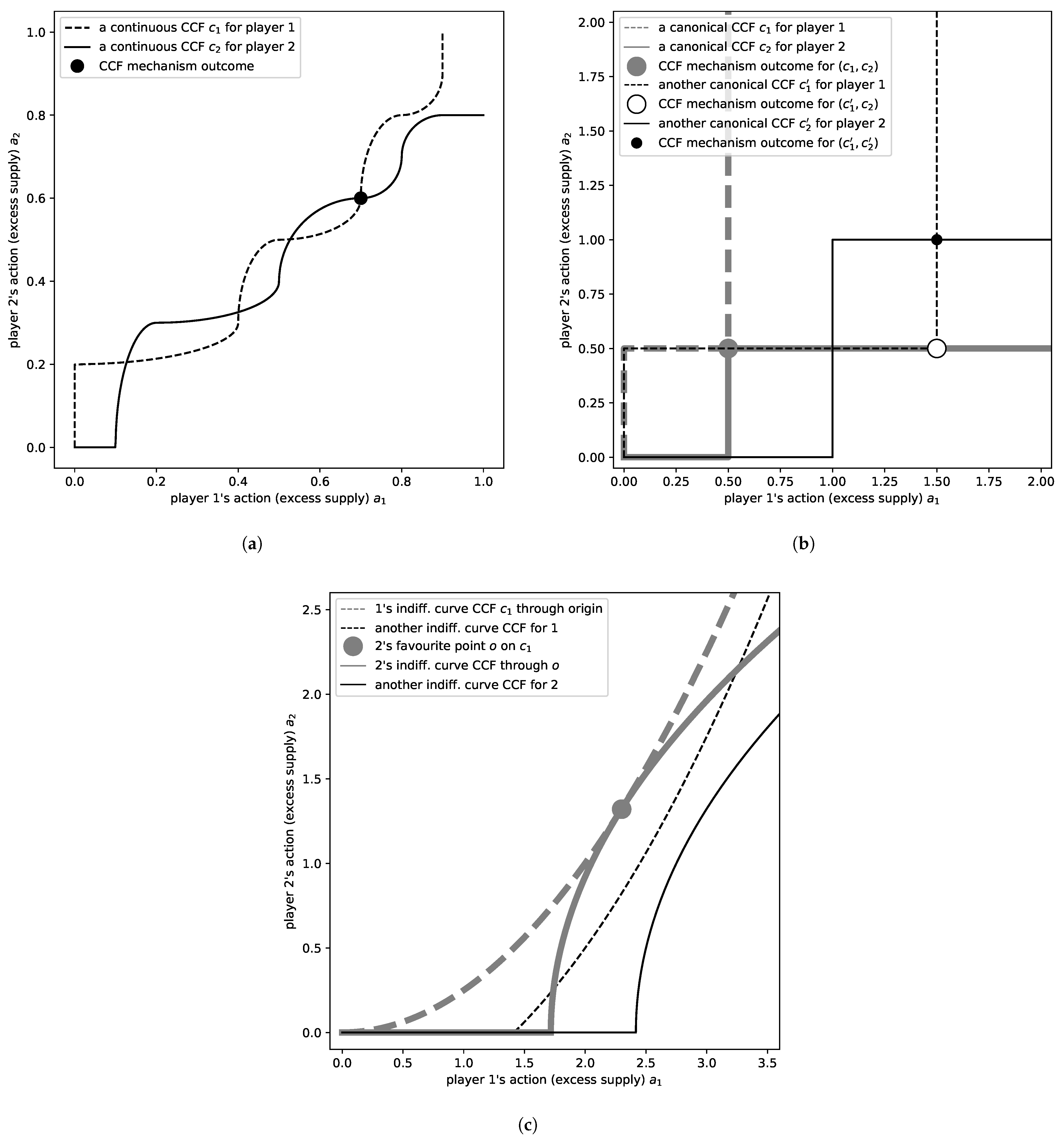
Figure 1. Examples of conditional commitment functions and CCF mechanism outcomes for two players. CCFs for player 1 are dashed, while those for player 2 are solid. (a) A continuous CCF for each player. The solid line (CCF c 2 for player 2) shows how much player 2 is willing to supply depending on player 1’s supply. The mechanism picks their uppermost intersection. (b) Two ‘canonical’ CCFs (i.e., simple step functions) for each player. The pair ( c 1 , c 2 ) only meets in the origin, which is, hence, their outcome. All other pairs meet or intersect at some positive excess supplies (dots). (c) Two indifference function CCFs for each player. The thick gray pair meets at the origin and at a Pareto-efficient point. Other pairings meet only at the origin, or at the origin and two further points.
Games 16 00058 g001
Figure 2. Core of the public goods problem of reducing output in a Cournot oligopoly with 3 firms (inverse demand function P ( y 1 + y 2 + y 3 ) = 4 y 1 y 2 y 3 , constant marginal costs of unity, Cournot point y i 0 = 3 / 4 , and output reductions a i = 3 / 4 y i ). The large dashed triangle is the Pareto-efficient surface (where a 1 + a 2 + a 3 = 3 / 4 ). The small inner dashed triangle contains the mutually profitable Pareto-efficient points (where also a i 3 / 8 ), each of which is supported by a Nash equilibrium in CCFs. The light hexagon is the core of the cooperative version of the underlying output reduction game (where also a i + a j 21 / 32 ). Each point in the core is supported by a strong Nash equilibrium in CCFs. The dark surface shows a canonical equilibrium CCF for firm 3 and a chosen efficient output reduction of a = 3 / 4 y = ( 0.3 , 0.25 , 0.2 ) (dotted lines emphasize where the step occurs).
Games 16 00058 g002
Figure 3. (Color online only) Learning strong equilibria and core outcomes in a public goods problem with three players. Starting with some CCF profile, players iteratively update their CCF to one that passes through their favourite point on all other players’ current CCFs and lies on or below their indifference curve through that point. If players “satisfice” by submitting indifference curves as their CCF, they usually converge after just one round, either to a corner (big dark dots (blue), if starting from zero CCFs) of the core (thick dark lines (blue): core boundaries, additional dashed lines: curvature on core manifold) or to some other core points (light dots (green), if starting from nonzero CCFs). When choosing CCFs properly below their indifference curves, they take longer (here shown: 30 rounds) to converge to the core (thin lines, smaller dark dots).
Games 16 00058 g003
Disclaimer/Publisher’s Note: The statements, opinions and data contained in all publications are solely those of the individual author(s) and contributor(s) and not of MDPI and/or the editor(s). MDPI and/or the editor(s) disclaim responsibility for any injury to people or property resulting from any ideas, methods, instructions or products referred to in the content.