Abstract
This paper delves into a multi-player non-renewable resource extraction differential game model, where the duration of the game is a random variable with a composite distribution function. We first explore the conditions under which the cooperative solution also constitutes a Nash equilibrium, thereby extending the theoretical framework from a fixed duration to the more complex and realistic setting of random duration. Assuming that players are unaware of the switching moment of the distribution function, we derive optimal estimates in both time-dependent and state-dependent cases. The findings contribute to a deeper understanding of strategic decision-making in resource extraction under uncertainty and have implications for various fields where random durations and cooperative strategies are relevant.
1. Introduction
Non-renewable resource extraction inherently involves strategic conflicts among multiple stakeholders operating under profound uncertainties. As demonstrated in Epaulard (1998), uncertainties regarding resource stock and technological progress profoundly affect extraction paths and decision-makers’ intertemporal decisions, adding more complex dimensions to this field full of strategic conflicts and uncertainties. Differential games, as mathematical frameworks capturing strategic interactions over time, offer powerful tools to model these conflicts Isaacs (1999). Traditional formulations of such games usually assume a fixed game duration (finite time duration) or rely on an infinite time duration. However, real-world scenarios related to non-renewable resource extraction, including equipment failures, policy shifts and environmental disruptions, introduce duration uncertainty. In these cases, the duration of the game cannot be determined a priori and depends on a number of unknown factors. This type of uncertainty gives rise to the fascinating field of differential games with random duration. The random nature of the duration of the game affects the optimal strategies of the players. Understanding this process is critical to developing decision-making mechanisms under uncertainty.
This class of games was first introduced in Petrosjan and Mursov (1966), which studied differential zero-sum games with terminal payoff at a random time horizon. Subsequently, Boukas et al. (1990) conducted a general study on an optimal control problem with random duration. The study of cooperative and non-cooperative differential games with random duration was continued by Shevkoplyas and Petrosyan in Petrosjan and Shevkoplyas (2003) and Shevkoplyas (2014). The form of integral payoff in differential games with random duration was investigated in (E. Gromova & Tur, 2017; Shevkoplyas & Kostyunin, 2013). This class of games was further extended to the case where the distribution function of the random terminal time of the game has a composite form (Gromov & Gromova, 2014, 2017). Specifically, it was assumed that the probability density function of the terminal time may change depending on certain conditions, which can be expressed as a function of time and state. This modification of games can be particularly useful in environmental models due to potential environmental disasters and climate change, as well as in technical models accounting for equipment failures or different modes of technical equipment operation. The study of such models was continued in Zaremba et al. (2020) for discontinuous distributions and in Balas and Tur (2023) for the case of feedback strategies. In parallel, Wu et al. (2023) focuses on sustainable optimal control for a switched pollution-control problem with random duration.
As mentioned above, incidents such as equipment failures may occur during resource extraction, causing switches in the game’s dynamic system. This can lead to changes in aspects of the game, including its payoff structure, state equations, or termination conditions. Stuermer and Schwerhoff (2015) studied how the geological distribution of the non-renewable resource interacts with technological change. The modelling of emission-reduction technology adoption as an endogenous threshold-triggered switch is presented in Parilina et al. (2024). The establishment of political regime switches as drivers of extraction voracity in non-renewable resources is addressed in Van der Ploeg (2024). The synthesis of stochastic equipment failures and periodic purification switching, along with the proof that pollution states converge to unique hybrid limit cycles, is conducted in Wu et al. (2025b). Additionally, the study of an multi-player hybrid pollution-control problem that considers switching behavior and uncertain game duration is reported in Wu et al. (2025a). The empirical validation of phase-specific efficiency switching in R&D competition, as well as the confirmation of the regime-dependent nature of duration effects, is carried out in Huang (2024). While existing studies have advanced the understanding of uncertainty and switching in resource-related games, they often lack a targeted analysis of how such integration operates in multi-player non-renewable resource extraction scenarios, leaving room to explore unaddressed problems like unknown distribution switching moment estimation.
In this paper, we consider a model of non-renewable resource extraction by multiple participants with random duration. The peculiarity of the model under consideration is that the distribution of the random terminal time of the game is composite. The first problem we address is the need to verify the preservation of the property proved in Dockner (2000) for a new formulation of the problem. In Dockner (2000), conditions were obtained under which the cooperative solution is also a Nash equilibrium in a similar problem with fixed duration. Our goal is to obtain similar conditions for a problem with a random duration and composite distribution. Furthermore, under the assumption that the players do not know the moment of switching of the distribution function, we study the problem of obtaining an optimal estimate of this unknown moment, as in Ye et al. (2024). Notably, a distinct model featuring random initial times of player entry is presented in E. V. Gromova and López-Barrientos (2016). While their work focuses on HJB equations and imputation distribution procedures for cooperative solutions under uncertain start times, our model addresses fundamentally different challenges: random terminal times with composite distributions and unknown switching mechanisms. This distinction positions our work as advancing the theoretical frontier in duration uncertainty rather than entry uncertainty, with direct implications for sustainability planning under environmental disruptions. Additionally, we derive optimal estimates in state-dependent cases. By delving into these aspects, we strive not only to enhance the theoretical framework of differential games in non-renewable resource extraction but also to offer practical strategies that can assist industry stakeholders in making more informed decisions. A comparative summary of our work alongside key related works is provided in Table A1 of the Appendix A.
This paper makes the following pivotal contributions:
- The construction of optimal cooperative and Nash equilibrium strategies of players in the differential non-renewable resource extraction game with a composite distribution function of the game’s random duration.
- The derivation of sufficient conditions under which the cooperative solution constitutes a Nash equilibrium within this model.
- The definition of the optimal estimation of unknown parameters in a differential game of non-renewable resource extraction.
- The development of a method of constructing the optimal estimation of unknown parameters.
- Optimal parameter estimates for both time-dependent and state-dependent cases.
This paper is organized as follows. In Section 2, we present the formulation of the problem. Section 3 proves that, in this model, the cooperative solution is a Nash equilibrium under certain conditions. Assuming that the players do not know the switching moment of the distribution function, we obtain the optimal estimate in the time-dependent case in Section 4 and Section 5. In Section 6 and Section 7, the optimal estimate in state-dependent case is obtained. In Section 8, we present a detailed example related to real-world oil extraction field development. Finally, in Section 9, we present our conclusion.
2. Problem Statement
We first summarize all key parameters of the model, along with their definitions, in Table 1 for reference.

Table 1.
Summary of model parameters.
Consider an n-player differential game of non-renewable resource extraction. The duration T of the game is a random variable following a ceratin distribution, whose cumulative distribution function is assumed to be an absolutely continuous nondecreasing function. Correspondingly, we adopt two distinct exponential cumulative distribution functions: describes the termination probability before the switching moment , and describes that after . This composite structure captures a system where hazard rates change from to .
At the switching moment , the left limit must be equal to the function value:
Assume an exponential structure when :
According to continuity, we have
i.e.,
we can obtain
Therefore, the duration T of the game has a composite cumulative distribution function:
Let denote the state variable representing the resource stock available for extraction at time t. The dynamics of the stock are shown by the following differential equation with the initial condition :
Here, denotes the extraction effort of player i at time t, and the coefficient is used to convert the effort of the i-th player into the extraction intensity. In accordance with the physical nature of the problem, we impose the constraints that and for all . Moreover, if , then the only feasible rate of extraction is for all . To simplify the notation, we denote . We consider the problem within the framework of open-loop strategies.
The expected integral payoff of player i, is evaluated by the following formula:
where . According to Shevkoplyas and Kostyunin (2013), Equation (3) can be written as follows:
In this study, the model aims to represent a typical dynamic decision-making problem faced by a coalition extracting a non-renewable resource (e.g., petroleum, natural gas, or mineral resources). Player i’s extraction effort can be interpreted as its invested capital, equipment, or number of drilling rigs. The coefficient characterizes player i’s technical efficiency in extraction; a higher value implies a greater extraction intensity for the same level of effort. The parameter captures the diminishing marginal returns of capital investment, a common assumption in resource economics. The random duration T could represent the time of resource exhaustion or the random time at which extraction activities are forcibly terminated due to external uncertainties such as risks of accidents and technical failures, economic constraints, new environmental policies, or technological revolutions. Thus, each player’s objective is to maximize their expected total payoff under the dual constraints of dynamic resource depletion and future uncertainty.
We hypothesize that players cooperate so as to achieve the maximum total payoff:
The optimal control problem can be divided into two sub-problems, corresponding to intervals and . Over every interval, we employ the Pontryagin maximum principle Pontryagin (2018).
- On the intervalThe Hamiltonian function is written aswhere is the adjoint variable.The optimal controls are obtained from the first-order optimality conditions :The second derivative of ensures that the obtained optimal controls are maximumThe equation for the adjoint variable takes the following formfrom which we obtain . Using transversality condition , we have the following form for the optimal trajectory on the interval :where .
- On the intervalIn the same way, we define the Hamiltonian functionThe optimal controls are obtained from the first-order optimality conditionsThe canonical system issubject to the boundary condition . We can obtain that . By leveraging the initial condition , we have the following form for the optimal trajectory on the interval :where , which is obtained using the condition .
The optimal cooperative strategies have the following form:
The cooperative trajectory, corresponding to (7), takes the following form:
The total payoff is
3. Nash Equilibrium
In the work by Dockner (2000), an intriguing question regarding the non-renewable resource extraction game was considered. Specifically, it was investigated whether the cooperative solution in this game can be achieved as a Nash equilibrium of a non-cooperative game. It turns out that the answer depends on the parameter values of the models. We also study this question for a game with random duration. As is standard in optimal control theory with a random horizon, the expectation involved in the game’s objective function can be transformed into an equivalent deterministic problem. Although the model’s duration T is random, the verification of the Nash equilibrium, which specifically involves ensuring no player has an incentive to unilaterally deviate from their strategy, leads to a deterministic optimal control problem for any deviating player. Theorem 1 shows the results obtained.
Theorem 1.
If , and for each player the inequality
is satisfied, then the cooperative solution in this game is a Nash equilibrium.
Proof of Theorem 1.
Suppose that player i deviates from the optimal cooperative behaviour using strategy . It is worth noting that if, under the situation , the resource is not exhausted by some finite point in time, then we have
for . This indicates that player i cannot achieve a higher payoff in this situation compared to the situation , as such an outcome would contradict the fact that the sum of players’ payoffs is maximized in the situation . Accordingly, a deviation from can be beneficial for player i only if, in the situation , the resource is exhausted by some time .
- First, consider the case where .Player i solves the following optimization problem:Let further denote the solution to (9). To determine , consider the Hamiltonian function for player i:By solving the respective canonical system, we obtainwhere .Thus, the corresponding value of the payoff function of player i isThen, we solve the problem .Find the first derivative of with respect to the variable :Note that , . If , then . So, . And if also , then .It can be concluded that if and , thenand
- Now consider the case where .Player i solves the following optimization problem:Let further denote the solution to (11). The corresponding trajectory isWe construct the Hamiltonians for the intervals and , respectively.Using the boundary conditions , , , , the solution can be obtainedwhere .The corresponding value of the payoff function of player i isIts first derivative over isNote that if , then , since and . Furthermore, if , then .It can be concluded that if and , thenTherefore, is an increasing function with respect to a variable .
Since , we conclude that the payoff of player i in the case is no more than his payoff in the case . Taking into account the increase in the function with respect to variable , and the fact that
we conclude that that if and , then for any finite value of ,
This means that no player i benefits from deviating from the cooperative trajectory, i.e., the cooperative solution in this game is a Nash equilibrium. □
This Theorem has significant practical implications. Its conditions and indicate that whether the cooperative solution can be a Nash equilibrium depends on three key factors: the hazard rates and , the marginal returns rate , and the technical efficiency of other players within the coalition. In practical resource extraction scenarios, this implies that, for a coalition to maintain stability, two prerequisites must be met. On the one hand, the risk of unexpected project termination in the early stage (before ) must be significantly higher than that in the later stage (after ). On the other hand, the technical efficiencies among coalition members must not differ excessively. Alternatively, if there are technologically advanced players, the effective benefit space must be large enough to suppress their incentive to unilaterally expand production and violate the cooperative agreement.
4. Time-Dependent Case
Let us now focus on the scenario where for all and . It is worth noting that for such parameter values, the condition stated in Theorem 1 holds only if . Nevertheless, for the sake of generality, we consider the problem in general for any number n. Although these parameter assignments are hypothetical, their values and relative relationships refer to stylized facts in resource economics to ensure the numerical results exhibit economic rationality.
Suppose that players do not have information about the exact value of the switching moment . They use an estimated switching moment of the switching moment in the control (7) instead of the exact value . This estimation arises due to the inherent uncertainty in the system and the lack of precise information. The exact value of is not directly observable, as it is influenced by multiple factors, including the dynamic interactions among players, system parameters, and external disturbances. Players use based on available information, historical data, or heuristic predictions, which serves as a reasonable approximation under these uncertain conditions.
Then, their controls have the following form:
For convenience, we denote the control of player i on the interval as and the control on the interval as .
The trajectory corresponding to these controls is
The form of players’ payoff in this scenario depends on the relationship between the values of and , which is expressed as follows:
- If , the total payoff has the following form:
- If , the total payoff has the following form:
The subsequent discussion focuses on the optimal determination of .
5. Optimal Estimate
To minimize potential risks, players may reach an agreement on a guess , which minimizes the worst-case loss. Consequently, the following minimax problem needs to be solved:
where is the estimated value of the switching moment, and is the actual value.
Denote . The following theorem provides a solution.
Theorem 2.
If , then the optimal estimate of the unknown switching moment that solves (16) is
where p is the solution of the equation
Proof of Theorem 2.
- First, we consider the maximization problem which can be rewritten asConsider the behaviour of functions and to solve the maximization problem.
- When ,Note that if and , thenRefer to Appendix B for the proof of this fact.It can be concluded from this that for and . This means that is a decreasing function of when ; then,
- When ,Note that if and , then (see Appendix C)Therefore, for and . This means that is an increasing function of when ; then,
Let , . - Then, the problem (16) is transformed into the following:Note that is an increasing function and is a decreasing function (see the proof in Appendix D). Given that and , it can be deduced that Equation has only one root. Considering the behavior of these two functions, we can conclude that this root is the point of the minimum of the upper envelope of and graphs (the point of their intersection). This means that this root is the solution to the problem (16).To find the root, we need to solve the following:Let , , then (17) can be transformed into
This concludes the proof. □
To illustrate the result of Theorem 2, we present a numerical example with the following values of parameters: , , , . Figure 1 shows the graphs of and under these conditions. It can be observed that the intersection point of these graphs corresponds to the minimum of their upper envelope.
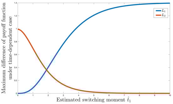
Figure 1.
Illustration of Theorem 2.
Finally, Table 2 shows the optimal estimates for different values of the parameter m. Figure 2 shows the maximum difference function and under these m values. The visualization results clearly reveal the mapping relationship between system parameters and functional behavior. Analysis demonstrates that m, as a key regulatory parameter, significantly influences the morphology of functions and and their intersection point: as m decreases, the intersection point of the two functions continuously moves upper-right, the optimal switching time increases substantially, and the corresponding function value also rises. This sensitivity analysis provides an intuitive basis for parameter optimization, indicating that system performance can be precisely modulated at different operating points by adjusting m.
Table 2.
Optimal estimates for different values of m.
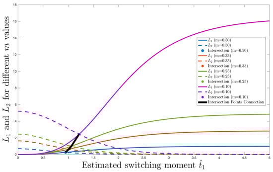
Figure 2.
Illustration of Table 2.
In the context of resource extraction, the switching moment can be interpreted as the anticipated time of a significant event, such as the enactment of new environmental regulations, the expected adoption time of a substitute technology, or a predicted market price inflection point. This time is unknown to the extractors due to incomplete information. The optimal estimate provided by Theorem 2 offers extractors a robust forecasting and decision-making tool. It also shows that is related to the parameter m, which is the hazard rate ratio between the time before and after the switch. Employing this estimate minimizes potential losses in the worst-case scenario, even if prediction errors exist, which is crucial for long-term investment and extraction planning under uncertainty.
6. State-Dependent Case
Following (Gromov & Gromova, 2014, 2017) and Balas and Tur (2023), we now assume that the stock level of the resource can influence the probability of a regime shift. Consequently, the switching does not occur at a fixed point in time but is triggered when a certain condition on the trajectory is satisfied. Within the framework of the model under consideration, such a condition could be the attainment of a predetermined level of resource stock.
Assume that is fixed, with . The switching moment for the composite distribution function (1) is determined by the condition .
Consider the Hamiltonian (6) in the interval with boundary conditions , , and the Hamiltonian (5) in the interval with boundary condition , along with the transversality condition , players’ controls are obtained in the following form:
To find the optimal solution, we also need to solve the following problem:
where
The optimal switching moment is:
In summary, the cooperative trajectory and the optimal cooperative controls at intervals and have the following form:
And the total payoff
7. Information Uncertainty
Suppose now that the value of is unknown to the players. They use instead of . Then, their strategies are
where
The corresponding trajectory has the following form:
To find the optimal estimate of , which minimizes the worst case possible loss in accordance with (16), we consider the minimax problem:
First, consider the maximization problem, which can be reformulated as
- When , we have , since the resource diminishes over time, where is the switching time of the composite distribution function.The value of could be obtained from Equation , i.e.,We can getand then the total payoff isHere, . We limit our analysis to the case of .Denote . Note thatsince function is increasing over when .
- When , we have , where could be obtained from Equation , i.e., . We can obtainThenDenote . In order to find , we need to solve , where changes the sign from positive to negative at this point. Let . Then, is the root of the following equation:For this equation takes the following form:and
Now, problem (23) could be rewritten as follows:
Let us demonstrate the numerical solution of this problem with different values of m.
An illustration of the solution for is provided in Figure 3. We assume , , for the case shown on the left side of Figure 3. And, , , for the right side of Figure 3. Interestingly, a rather general result is obtained that does not depend on the values of the parameters n and . In all cases, for , the optimal estimate will be .
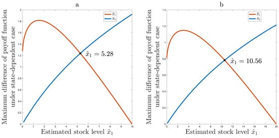
Figure 3.
(a) Optimal solution for , , , ; (b) Optimal solution for , , , .
Let’s continue with the parameters , , . The left side of Figure 4 shows the solution for . In this case, . For , we showed that . This is shown in the right side of Figure 4.
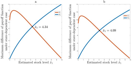
Figure 4.
(a) Optimal solution for ; (b) Optimal solution for .
Comparing the optimal estimation in the time-dependent and state-dependent cases, we can see that in the first case, the optimal estimation depends only on the values of parameters m and , whereas in the second case, it also depends on .
8. Example: Oil Extraction Field with Equipment Modernization
Consider three companies (players) operating symmetrically in a shared oil field with an initial stock of 100 million tons (i.e., ). These companies are aware that new technologies are being developed which have the potential to improve extraction processes and reduce the risk of catastrophic accidents. However, the exact timing of the implementation of these innovations remains uncertain.
Before this modernization (), the equipment is older and more prone to failures, leading to a higher risk of a catastrophic accident that would terminate extraction operations. After modernization (), the new, more reliable equipment significantly reduces this risk. Consequently, the hazard rate before modernization is higher than the hazard rate afterwards .
The technical efficiency parameters are set to be equal for all players due to symmetry: . The output elasticity is set to . The hazard rates are configured as for the high-risk period before modernization and for the lower-risk period after modernization.
The central question for the companies is to determine optimal extraction strategies under this operational risk uncertainty.
1. Time-dependent switching estimation
The optimal estimate for the switching moment (modernization time), , is derived from the model (substituting the parameter values )
2. State-dependent switching estimation
The optimal estimated switching moment occurs when the resource level reaches
Despite the planned modernization being 10 years away, the optimal robust strategy derived from our model suggests that the companies should behave as if the transition to the lower-risk environment will occur in approximately 5.29 years (time-dependent) or when the oil reserve depletes to about 43.4 million tons (state-dependent). This result indicates that optimal strategy requires adopting more conservative extraction measures in the near term to mitigate the higher operational risks associated with the older equipment, rather than waiting for the scheduled modernization.
This example demonstrates how our model provides practical insights for resource extraction industries facing operational risk uncertainties, enabling more informed decision-making for equipment upgrade scheduling and risk management strategies.
9. Conclusions
A model of multi-player non-renewable resource extraction with a random duration is considered. It is assumed that the distribution of the random duration of the game is composite. The conditions under which the cooperative solution is also a Nash equilibrium are obtained. For the case where players do not know the exact moment of switching of the distribution function, the optimal estimate of this unknown moment is obtained for both the time-dependent and state-dependent cases.
Furthermore, this research offers practical insights for managing non-renewable resources, suggesting that the stability of extraction coalitions depends on the balance of technical efficiencies among players and hazard rates, and provides a robust tool for estimating uncertain future policy or market shifts.
However, this study has limitations, as our model relies on specific assumptions regarding the functional form of the composite distribution and player preferences, which may not fully capture the complexity of real-world scenarios. While providing a foundational framework, these limitations also open several promising research avenues. Future work should extend beyond our assumptions by investigating more general distribution forms for the random duration and by incorporating asymmetric information and heterogeneous among players, particularly use a Bayesian Nash equilibrium approach. Other promising directions include endogenizing the switching mechanism itself and exploring more complex preference structures.
Author Contributions
Methodology, P.Y. and A.T.; investigation, Y.W.; writing—original draft preparation, P.Y.; writing—review and editing, A.T. All authors have read and agreed to the published version of the manuscript.
Funding
The work of the second author (Anna Tur) was supported by the Russian Science Foundation grant number 24-21-00302, https://rscf.ru/en/project/24-21-00302/ (accessed on 21 September 2025).
Data Availability Statement
No new data were created or analyzed in this study.
Conflicts of Interest
The authors declare no conflicts of interest.
Appendix A
Table A1 presents a comparative summary of our study alongside the main relevant literature.
Table A1.
Comparison of this study with relevant literature.
Table A1.
Comparison of this study with relevant literature.
| Duration | Switching | Uncertainty | |
|---|---|---|---|
| Petrosjan and Shevkoplyas (2003), Shevkoplyas (2014), Shevkoplyas and Kostyunin (2013) | Random | × | terminal time |
| Gromov and Gromova (2014), Zaremba et al. (2020), Wu et al. (2023, 2025a) | Random | switching of distribution function | terminal time |
| E. Gromova and Tur (2017) | Random | switching of distribution function | terminal time and initial time |
| Balas and Tur (2023) | Random | switching of distribution function, different switching rules | terminal time |
| Wu et al. (2025b) | Random | switching of distribution function, regime shift | terminal time |
| Gromov and Gromova (2017) | Infinite | different switching rules | × |
| Stuermer and Schwerhoff (2015) | Infinite | technological change | × |
| Parilina et al. (2024) | Infinite | switching of variables, reputation, emission | × |
| Van der Ploeg (2024) | Infinite | regime switches | regime switch time |
| E. V. Gromova and López-Barrientos (2016) | Infinite | changes in the number of players and game model | initial time |
| Huang (2024) | Finite | switching of distribution function | time of the completion of the project |
| Ye et al. (2024) | Finite | utility function switching | switching moment |
| This study | Random | switching of distribution function, different switching rules | terminal time and switching moment |
Appendix B
In this appendix we are going to prove that if and , then
Denote , .
Note that if and , then is a concave-down increasing function of , since and . In contrast, is a concave-up increasing function of , since and . It can also be observed that . Figure A1 is an illustration of the behavior of the functions and .

Figure A1.
Illustration of the behavior of and .
Thus, to prove the inequality (A1), it is sufficient to prove .
To achieve this, consider the following difference:
and its first partial derivative
Let us define . Note that
This means that is an increasing function of . Moreover, since , it follows that for .
Then if , which means that is an increasing function of . Additionally, since , it follows that if . From this we can directly conclude that . This concludes the proof of the inequality (A1).
Appendix C
In this appendix we are going to prove that if and , then
For simplicity, rather than directly proving inequality (A2),we will instead demonstrate the equivalent inequality:
Consider the difference:
Let represent the numerator of this fraction, i.e.,
The derivative of with respect to is given by
It is evident that when , with equality occurring only when . This implies that is a decreasing function of . Since , we can conclude that if . Consequently, we have:
which proves the inequality (A2).
Appendix D
In this appendix we are going to prove that if , then is an increasing function, here
Its derivative with respect to is
where .
Note that and
when , since . It follows that and when and . Then we can conclude that is an increasing function of . In the same way, it can be proved that is a decreasing function of .
References
- Balas, T., & Tur, A. (2023). The Hamilton–Jacobi–Bellman equation for differential games with composite distribution of random time horizon. Mathematics, 11(2), 462. [Google Scholar] [CrossRef]
- Boukas, E. K., Haurie, A., & Michel, P. (1990). An optimal control problem with a random stopping time. Journal of Optimization Theory and Applications, 64(3), 471–480. [Google Scholar] [CrossRef]
- Dockner, E. (2000). Differential games in economics and management science. Cambridge University Press. [Google Scholar]
- Epaulard, A., & Pommeret, A. (1998). Does uncertainty lead to a more conservative use of a non renewable resource? A recursive utility approach. Journées de l’AFSE sur Économie de l’Environnement et des Ressources Naturelles, 11–12. Available online: https://www.researchgate.net/publication/228912969_Does_uncertainty_lead_to_a_more_conservative_use_of_a_non_renewable_resource_A_recursive_utility_approach (accessed on 21 September 2025).
- Gromov, D., & Gromova, E. (2014). Differential games with random duration: A hybrid systems formulation. Contributions to Game Theory and Management, 7, 104–119. [Google Scholar]
- Gromov, D., & Gromova, E. (2017). On a class of hybrid differential games. Dynamic Games and Applications, 7(2), 266–288. [Google Scholar] [CrossRef]
- Gromova, E., & Tur, A. (2017, October 26–28). On the form of integral payoff in differential games with random duration. 2017 XXVI International Conference on Information, Communication and Automation Technologies (ICAT) (pp. 1–6), Sarajevo, Bosnia and Herzegovina. [Google Scholar]
- Gromova, E. V., & López-Barrientos, J. D. (2016). A differential game model for the extraction of nonrenewable resources with random initial times—The cooperative and competitive cases. International Game Theory Review, 18(2), 1640004. [Google Scholar] [CrossRef]
- Huang, X. (2024). Differential games of R&D competition with switching dynamics. Contributions to Game Theory and Management, 17, 38–50. [Google Scholar]
- Isaacs, R. (1999). Differential games: A mathematical theory with applications to warfare and pursuit, control and optimization. Courier Corporation. [Google Scholar]
- Parilina, E., Yao, F., & Zaccour, G. (2024). Pricing and investment in manufacturing and logistics when environmental reputation matters. Transportation Research Part E: Logistics and Transportation Review, 184, 103468. [Google Scholar] [CrossRef]
- Petrosjan, L. A., & Mursov, N. V. (1966). Game theoretical problems in mechanics. Lithuanian Mathematical Journal, 6(3), 423–433. [Google Scholar] [CrossRef]
- Petrosjan, L. A., & Shevkoplyas, E. V. (2003). Cooperative solution for games with random duration. Game Theory and Applications, 9, 125–139. [Google Scholar]
- Pontryagin, L. S. (2018). Mathematical theory of optimal processes. Routledge. [Google Scholar]
- Shevkoplyas, E. V. (2014). The Hamilton-Jacobi-Bellman equation for a class of differential games with random duration. Automation and Remote Control, 75, 959–970. [Google Scholar] [CrossRef]
- Shevkoplyas, E. V., & Kostyunin, S. Y. (2013). A class of differential games with random terminal time. Game Theory and Applications, 16, 177–192. [Google Scholar]
- Stuermer, M., & Schwerhoff, G. (2015). Non-renewable resources, extraction technology, and endogenous growth. FRB of Dallas Working Paper, No. 1506. Federal Reserve Bank of Dallas. [Google Scholar]
- Van der Ploeg, F. (2024). Benefits of rent sharing in dynamic resource games. Dynamic Games and Applications, 14(1), 20–32. [Google Scholar] [CrossRef]
- Wu, Y., Tur, A., & Wang, H. (2023). Sustainable optimal control for switched pollution-control problem with random duration. Entropy, 25(10), 1426. [Google Scholar] [CrossRef] [PubMed]
- Wu, Y., Tur, A., & Ye, P. (2025a). Sustainable cooperation on the hybrid pollution-control game with heterogeneous players. arXiv, arXiv:2504.12059. [Google Scholar] [CrossRef]
- Wu, Y., Tur, A., & Ye, P. (2025b). Sustainable solution for hybrid differential game with regime shifts and random duration. Nonlinear Analysis: Hybrid Systems, 55, 101553. [Google Scholar] [CrossRef]
- Ye, P., Tur, A., & Wu, Y. (2024). On the estimation of the switching moment of utility functions in cooperative differential games. Kybernetes. [Google Scholar] [CrossRef]
- Zaremba, A., Gromova, E., & Tur, A. (2020). A differential game with random time horizon and discontinuous distribution. Mathematics, 8(12), 2185. [Google Scholar] [CrossRef]
Disclaimer/Publisher’s Note: The statements, opinions and data contained in all publications are solely those of the individual author(s) and contributor(s) and not of MDPI and/or the editor(s). MDPI and/or the editor(s) disclaim responsibility for any injury to people or property resulting from any ideas, methods, instructions or products referred to in the content. |
© 2025 by the authors. Licensee MDPI, Basel, Switzerland. This article is an open access article distributed under the terms and conditions of the Creative Commons Attribution (CC BY) license (https://creativecommons.org/licenses/by/4.0/).