Abstract
Hierarchies are common in political settings. From judges to elected politicians, as well as from activists to bureaucrats, political agents compete for promotion to higher positions. This paper studies political tournaments and their impact on two aspects of political performance: accountability and selection. While larger tournaments discourage effort, they improve selection. We also discuss the optimal design of tournaments as a function of the principal’s objectives and the features of the environment. We find that tournaments of size two (such as two-candidate elections) are generally suboptimal. Our analysis also highlights that increased desirability of promotion always increases effort but can reduce the optimal tournament size under certain conditions. We also present a range of other comparative statics.
1. Introduction
Hierarchies are common in political settings. Electoral careers often begin at the local level and progress to the provincial or national level (Myerson, 2006). Judges move through the various strata of the judicial system (Epstein et al., 2003). Authoritarian leaders fill vacancies by drawing on administrators at lower levels (Lu & Landy, 2014). Bureaucrats are promoted through various grades of pay and responsibility (Cameron et al., 2013). Political parties have their own set of rules and structures, with members competing for positions on party lists or in leadership roles (Michels, 1915). Legislators seek ministerial positions (Eggers & Spirling, 2016) or assignments to desirable committees (Fong & McCrain, 2024; Groseclose & Stewart, 1998). Even electoral campaigns can be understood in this light, where candidates seek to win office by proving themselves in the eyes of a voter.
Hierarchical structures allow a principal (e.g., a party leader, the president, or an authoritarian ruler) to select the most capable agent (legislator, bureaucrat, or local administrator) to fill a vacant position (cabinet post, agency head, or provincial position). Hierarchies thus presuppose the possibility of promotions. From the perspective of agents, promotions are prizes to be won by besting fellow contestants. From the perspective of the principal, promotions are a way to select the most competent agents while also incentivizing effort. Promotion-based hierarchies are thus best understood as tournaments with a twist.
Rather than just being about incentives—the focus of a large portion of literature since Lazear and Rosen (1981)—the tournament we study also serves as a tool for selection. In our setting, effort is a by-product of selection. Effort occurs as an attempt to mislead the principal, which is an attempt that fails in equilibrium. We emphasize that, within the class of symmetric equilibria, the effort level is uniquely pinned down—something that is not guaranteed in all tournament models that rely on effort incentives. Furthermore, the unique equilibrium level of effort we obtain is equal to the highest level of effort agents exert in traditional tournament models.
Our first key result shows that selection in promotion-based tournaments comes at almost no cost. The principal can use a tournament to select the ablest agent and still obtain a very high level of effort from everyone involved. Yet, this does not imply that selection and accountability—defined as the level of effort agents exert—always go hand in hand.1
Increasing the number of agents competing with each other can yield an accountability–selection tradeoff for the principal. Having more agents competing always improves the expected ability of the selected agent but also reduces the amount of effort each agent exerts. This has implications for the design of the optimal tournament (i.e., the number of participants allowed to compete), which is a question we briefly study at the end of our paper.
We show that in some settings (e.g., if the principal cares about average performance), a principal may choose to restrict the number of participants in a tournament to provide greater incentives for effort. Yet, we nonetheless find that whenever the principal cares about effort in addition to selection, tournaments with two competing agents are generally dominated by larger tournaments. This result suggests that two-candidate elections are suboptimal from the electorate’s perspective unless the cost of running larger elections is very high.
Our paper also provides a host of additional comparative statics—some are intuitive, while others are more subtle. Effort is increasing with the value of the prize (as agents find promotion more valuable) and decreasing with the heterogeneity of ability and the informativeness of agents’ outputs as signals of their skills (since in both cases, effort is less likely to determine promotion). In turn, selection always improves with the variance in agents’ types, as the principal only cares about the highest draw of ability. More surprisingly, perhaps, even though effort increases with the value of the prize, the optimal tournament size decreases with the desirability of promotion whenever the principal cares about the promoted agent’s effort. The key force behind this result is that the principal weighs the gain and loss of adding one competitor when designing a tournament. A higher prize exacerbates the negative effect on the effort of increasing the pool of competitors. In turn, greater desirability of promotion leads to a larger tournament when the principal cares about total effort, since a larger prize enhances the gain from increased size.
Literature Review. The theoretical analysis of tournaments is not new. Beginning with the seminal work of Lazear and Rosen (1981), tournament incentives have been studied extensively (see Waldman, 2013, for a review). Early results emphasized that tournaments are dominated by (sufficiently rich) contracts when it comes to incentive provision, since they introduce noise into compensation schemes (Green & Stokey, 1983).
Later studies justified tournaments as an optimal response to specific features of the environment, such as common shocks (Maskin et al., 2000) or commitment problems (Malcomson, 1986), or assumed a tournament and characterized the optimal prize structure (Krishna & Morgan, 1998, builds on Nalebuff & Stiglitz, 1983). Connelly et al. (2014) provided a useful review of the large literature on tournaments as a tool for accountability, from both a theoretical and an empirical angle.
For a long time, tournament models failed to consider selection. This was one of the critiques raised by Prendergast (1999). Since then, tremendous progress has been made in addressing this gap. While some works have focused exclusively on selection (e.g., Clark & Riis, 2001; Ryvkin, 2010), others, like us, have incorporated both effort and selection. Gürtler and Gürtler (2015) showed how two agents may be motivated to exert greater effort when they are known to have different average abilities. Höchtl et al. (n.d.) looked at a two-stage tournament and found that selection benefits from heterogeneous competitors competing early with each other. Levy and Zhang (2024) argue that, if agents are homogeneous in their ability, pooled contests (where all participants compete with each other) may be better than two-stage tournaments.
While these contributions are important, we advance the literature along two fronts. First, we return to the traditional model of the tournament (Höchtl et al., n.d.; Levy & Zhang, 2024, use a contest function) and solve a tournament game with promotion involving a large number of agents (Gürtler & Gürtler, 2015, whereas prior work only considered a two-agent tournament). Second, we discuss the gains and losses from increasing the size of the tournament, taking into consideration both accountability and selection.2
By considering accountability and selection, our work is related to agency models of elections (see Ashworth, 2012, for a review). Canonical political career concerns models (e.g., Ashworth, 2005) are, however, a special case of political tournaments in which only the performance of one agent is observed and compared to a benchmark. Our richer setup allows us to compare how electoral incentives differ from other types of tournaments and generate novel comparative statics relating the optimal size of a tournament to model parameters.
Further, while electoral accountability models focus on bottom-up accountability, promotion-based hierarchies are best understood as top-down accountability problems. Ghosh and Waldman (2010) studied how promotions can be used to screen agents. They focused on a one-to-one relationship between firm owners and workers and so had nothing to say about the size effect of promotion tournaments. Our approach, instead, is rooted in the idea that top-down accountability is a many-to-one problem, and agents are rarely judged in isolation. Montagnes and Wolton (2019) and Wang et al. (2022) studied a related question. However, they assumed that the principal has coarse information about her agents’ performances and emphasized the role of punishments (purges in authoritarian countries) rather than rewards.
2. Formal Model of Tournaments with Selection
We consider a one-period game with a principal and a set of available agents with cardinality . The principal first decides the number of agents to be considered for promotion to a unique higher-up position valued by all agents. The n randomly selected agents then compete by exerting costly effort to manipulate the principal’s promotion decision. We thus describe the subgame played by the selected agents as an n-agent tournament.
Each agent i is characterized by their ability . Following canonical models of tournaments (e.g., Lazear & Rosen, 1981) and career concerns models (e.g., Ashworth, 2005; Holmström, 1999), we assume that is unknown to all players at the beginning of the game. It is, however, common knowledge that for all , is independently and identically distributed (i.i.d.) over the interval (possibly unbounded) according to the cumulative distribution function (CDF) , with variance and symmetric and single-peaked probability density function (pdf) .3 We further assume that and are continuously differentiable (i.e., ). The principal cares about the promoted agent’s ability. She, however, only observes a noisy signal of agents’ skills before making her promotion decision for those considered for promotion; otherwise, she observes nothing. More specifically, an agent considered for promotion produces an output—denoted for all —which consists of the sum of the agent’s ability , their effort , and a noise (luck) term :
Effort is unobserved by the principal. As in career concerns models, agents try to manipulate the signal available to the principal. However, unlike career concerns models, n agents simultaneously compete for promotion by exerting effort. The noise term is also unknown to all players, but it is common knowledge that is i.i.d. over the interval (possibly unbounded) according to the CDF m with variance and symmetric and single-peaked pdf .4 Notice that the output function only incorporates independent shocks. This assumption is without loss of generality since, as extensively noted in the literature (e.g., Green & Stokey, 1983; Maskin et al., 2000), any shock that would similarly impact all agents would be differenced out by the principal, who evaluates agents on their relative rather than absolute performance.
An agent receives a payoff V if promoted and 0 if otherwise. The agent also pays a cost to exert effort and manipulate the signal available to the principal. We assume that is , increasing, and convex. Agent i’s utility function thus takes the following form (with being the indicator function equal to 1 if i is promoted):
The principal’s utility depends on both the ability of the promoted agent and the agents’ efforts. We assume that increasing the size of the tournament is costly, with the convex cost function . The principal’s utility can be represented as
where is the weight on agents’ effort, is a continuous function weakly increasing in all its arguments,5 and is an indicator function equal to 1 if i is promoted and 0 if otherwise.
To summarize, the timing of the game is as follows:
- Nature draws relative abilities () and noise () for each agent , and these values are unobserved by all players.
- The principal selects the number of agents to be considered for promotion, where . For notational convenience and without loss of generality, we assume that the first n agents are selected.
- Each selected agent i simultaneously chooses their effort .
- For each selected agent i, the output is observed by all players.
- The principal promotes one agent among the n selected agents. The game ends, and payoffs are realized.
The equilibrium concept is Perfect Bayesian Equilibrium in pure strategies. We focus on symmetric equilibria. Two well-known aspects of Perfect Bayesian Equilibrium are worth stressing: (i) All players consistently anticipate other players’ strategies so that (ii) agent i and the principal have the same expectation about agent j’s effort for all . Throughout, we posit variance parameters for ability and noise that place the game in the well-behaved region identified in the tournament literature—conditions under which a single symmetric equilibrium is generally obtained. We adopt that equilibrium for all subsequent analysis (This assumption is common in the literature; see Green & Stokey, 1983; Krishna & Morgan, 1998; Nalebuff & Stiglitz, 1983).6
As a preliminary, note that given the principal’s objective, she always promotes the agent with the highest expected ability. To form a correct assessment of agents’ skills, she adjusts for agents’ anticipated effort from the observed outputs. Since her anticipation is correct in equilibrium, we can study promotion and effort separately. We thus depart from the usual (backwards) order of analysis and focus first on agents’ effort and how it varies with the model parameters and the size of the tournament.
3. Agents’ Effort
We first consider effort in a tournament of size n. Agents not competing for promotion (i.e., agents ) do not exert any effort. Likewise, in a tournament of size one, agent 1 exerts no effort. Therefore, in what follows, we focus on tournaments of size at least 2. We introduce the following notation: let be the principal’s anticipation of j’s effort.
Agent is promoted if and only if the principal expects their ability to be the highest. This occurs whenever they produce the highest output net of anticipated effort, i.e., . Agent i, however, does not observe and must form beliefs about other agents’ performances based on (i) their anticipation of the realization of their ability () and luck () and (ii) their effort (). Denote as i’s anticipation of j’s effort for all . The probability that i is promoted given their output is . Imposing the assumption that anticipated efforts are consistent (i.e., ), this reduces to
Equation (4) highlights that only the joint effect of and enters into agent i’s assessment. Since the two random variables are independent, it is convenient to merge the terms into a ‘combined noise’ for all j. For each j, the combined noise is i.i.d. over () according to the CDF , with variance and pdf . Observe that due to the independence of and , is single-peaked and symmetric. Using the independence of ’s, the probability that i is promoted for a given output is thus .
Agent i, however, only chooses their effort, not their output , which corresponds to the sum of effort and their own combined noise . Since agent i correctly treats as a random variable, they maximize the following objective function (with the conditional operator over ):
Through standard maximization (our assumption on variances guarantees that the second-order condition holds), we can then characterize the agents’ effort.
Proposition 1.
There exists a unique equilibrium effort in pure strategies. The equilibrium effort is symmetric—denoted as —and characterized by the following equation:
Proof.
Proofs for this section are collected in Appendix A. □
Our next set of results establishes how the tournament structure—the value of the prize (V), the variance of the combined noise (), and the size of the tournament (n)—affects the equilibrium effort.
Proposition 2.
The equilibrium level of effort is as follows:
- (i)
- Decreasing in n (i.e., for );
- (ii)
- Strictly decreasing in ;
- (iii)
- Strictly increasing in V.
Points (ii) and (iii) of Proposition 2 are intuitive. As the prize becomes more attractive (the value of promotion V increases), agents have more incentive to exert effort. As the variance of the combined noise grows, effort is less and less likely to determine the outcome of the tournament. As a consequence, all agents have reduced incentive to exert effort.
The intuition for point (i) is more subtle. As the size of the tournament grows, competition to be promoted becomes more intense. Naive economic reasoning then suggests that effort should increase. This intuition fails to consider the effect of the combined noises on agents’ effort choices. When choosing their effort, agent i does not compare their output with every other agent’s. Rather, as explained above, they only take into account their best-performing competitor. As the number of competing agents increases, the combined noise associated with agent i’s best competitor becomes increasingly likely to take high values (more precisely, strictly first-order stochastically dominates for all ).
Better performance by the highest competitor alone, however, is not sufficient to discourage effort by agent . Indeed, agent i’s effort equates the marginal cost with the marginal gain in promotion probability. Their total winning probability has little effect on their effort choice. In turn, the marginal gain in promotion probability depends on the distribution of their own combined noise . Since is single-peaked and symmetric, agent i’s effort is more likely to be complemented by low (in absolute value) rather than large combined noise. Consequently, as the size of the tournament grows, the probability that their output is close to their highest competitor’s decreases, as does the likelihood that a marginal increase in effort significantly increases their promotion probability.
The reasoning above thus indicates that an agent’s performance decreases with the size of the tournament due to the combination of two effects. First, their highest competitor’s performance increases. Second, more effort is less and less likely to significantly impact their promotion probability. Absent either of these two effects, the size of the tournament has no impact on an agent’s effort choice.7 In particular, when is uniformly distributed so that all levels of combined noise are equally likely, the size of the tournament has no effect on agents’ effort.8
Figure 1 illustrates these scenarios. We display three pdfs of the combined noise : the pdf for agent i (in red, dotted), the pdf for the best competitor in a tournament of size 4 (blue, dashed), and the pdf for the highest competitor in a tournament of size 10 (black, plain). In Figure 1a, the of tournament participants is normally distributed (mean 0, variance ). In Figure 1b, the of participants is uniformly distributed (over ). For both distributions, agent i’s chances of winning are lower when there are 10 participants than when there are 4 participants in the tournament: The red curve crosses the blue dashed curve before the black curve and, as we noted, the best competitor’s pdf when is to the left of the best competitor’s pdf when (i.e., strictly first-order stochastically dominates ). Yet, agent i does not consider his total chances of winning when deciding their effort but the marginal change in winning probabilities. The increase in their chances of winning following greater effort is illustrated by the yellow filled zone when and the orange filled zone when in Figure 1a,b. With a singled-peaked distribution like the normal distribution, we can visually see that increased effort has a smaller effect on i’s winning chances when than when (the orange zone is smaller than the yellow zone). Hence, agent i has less incentives to exert effort in a larger tournament. In contrast, with the uniform distribution, the effect of increased effort is the same for both tournament sizes (the yellow zone and the orange zone have the same area). In this case, the incentive to exert effort is independent of the tournament size.
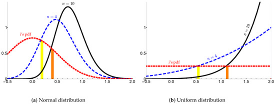
Figure 1.
Comparing distributions. The graphs display the pdf of for agent i and the pdf of for the best competitor for tournament of size 4 (dashed blue line) and size 10 (plain black line). (a) for all participants is normally distributed with mean 0 and variance . (b) for all participants is uniformly distributed over .
As Corollary 1 also shows, 2-agent and 3-agent tournaments yield the same equilibrium effort, as the negative effect of the highest competitor’s increased performance is counterbalanced by a positive effect of lower variance, which increases the marginal value of effort.
Corollary 1.
The equilibrium effort satisfies if and only if and there exists such that .
Without imposing additional conditions on the shape of agents’ cost function , we cannot characterize further features of equilibrium effort. Since effort is determined by the marginal cost, any second-order prediction depends on the third derivative of the cost function. In the next corollary, we instead examine certain properties of the marginal benefit of effort, which we denote as (see the right-hand side of Equation (6)).
Corollary 2.
The marginal benefit of effort satisfies the following properties:
- (i)
- Convex in n (i.e., for and ), strictly if for some ;
- (ii)
- Strictly convex in ;
- (iii)
- Neither concave nor convex in V.
Point (iii) follows from the risk neutrality of the agent. Any increase in the prize linearly increases the benefit from winning the tournament and, in turn, the marginal benefit of effort. Point (ii) follows from the effect of higher variance on . As increases, the pdf of the combined noise flattens, and an increase in effort becomes marginally more likely to affect the tournament outcome. This second-order effect attenuates the direct effect of variance identified above.
Point (i) indicates that the negative effect on incentives of increased tournament size on effort attenuates as the tournament grows larger. This arises because of the effect of adding one more agent on the highest performance (in expectation). The direct effect is that expected highest performance increases. However, this also implies, as a second-order effect, that higher and higher realizations of the combined noise are necessary to improve the highest performance. Since is single-peaked (i.e., low values of in absolute terms are more likely), such events are increasingly unlikely. Consequently, the expected highest performance increases at a decreasing rate with the number of participants. Since the marginal benefit of effort is inversely related to the highest performance of other agents, it is convex in n.
Figure 2 summarizes the results of this section. There, we display how the marginal benefit of effort () varies with the size of the tournament (left panel), the value of the prize V (middle panel), and the variance of the combined noise (right panel), assuming that both ability and luck are normally distributed. Figure 2a highlights that (i) the marginal benefit of effort (and thus the equilibrium effort itself) is the same for and tournaments, and (ii) the marginal benefit of effort is decreasing and convex nature in the number of participants. In Figure 2b, we see how the marginal benefit increases linearly with the value of the prize, whereas the marginal benefit of effort is decreasing and convex with the variance of , as shown in Figure 2c. In these last two figues, we also observe how the marginal benefit of effort is lower for large than for small tournaments.
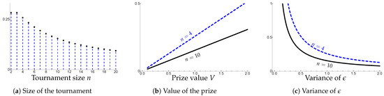
Figure 2.
Comparative statics on the marginal benefit. The graphs display the marginal benefit as a function of the tournament size (a), the prize (b), and the variance of (c). (b,c) we display the marignal benefit for a tournament of size 4 (blue dashed curve) and of size 10 (dark plain curve). (a,b) takes value one. (a,c) V takes value one. In all panels, is normally distributed with mean zero.
Having established the general properties of the marginal benefit of effort, we can provide some predictions for the effect of the tournament parameters on effort. The second-order effect of V on effort depends on the sign of . In turn, the equilibrium effort is convex for both and the number of agents n whenever is not too large.
4. Tournament and Selection
As highlighted by Equation (3), the principal cares not only about the agents’ effort (through ) but also about the ability of the promoted agent. Because all agents exert the same level of effort , the principal simply promotes the best performer. Further, since she correctly anticipates effort, she can recover the combined noise of the best performer, which is denoted as (i.e., ). From the principal’s perspective, the promoted agent’s expected ability—denoted as —is then, for a given output,
When deciding the tournament size, the principal can only condition her decision to select n agents on the expected realizations of agents’ ability and luck. From an ex ante perspective, the important statistic for the principal is
Our first result is quite intuitive. As the tournament size grows, the (ex ante) expected ability of the promoted agent increases. Given that effort does not affect the principal’s promotion decision, adding agents can only increase the probability that a large combined noise is realized. While effort declines in a larger tournament, selection strictly improves.
Proposition 3.
The ex ante expected ability of the promoted agent increases with the size of the tournament.
Additional conditions on the distribution of ability and luck are required to establish further properties of . As is common in the literature on career concerns, we impose that and are both normally distributed (i.e., and ). Under these assumptions, takes a very simple form: . Denoting , we obtain
Under the assumption of normality, we can provide a fuller picture of the impact of tournament characteristics on the ex ante ability of the promoted agent, which is defined as .
Proposition 4.
Suppose and are normally distributed. The ex ante expected ability of the promoted agent is defined as follows:
- (i)
- Strictly increasing in ;
- (ii)
- Strictly decreasing in .
- (iii)
- Strictly concave in n.
As the variance in abilities increases, extreme realizations of ability become more likely. Since the principal only cares about the highest realization, not the average of realizations, at the time of promotion, this always benefits the principal. In turn, when the variance of the noise component increases, high output is more likely to be due to luck than ability. This, therefore, tends to depress the expected ability of the promoted agent. Finally, the last point of the proposition indicates that the gain from adding contestants decreases with the size of the tournament. The logic is the same as for the convexity of effort in n. As the expected highest ability rises (i.e., increases with n), it becomes less and less likely that the ability of an additional agent will surpass .
Figure 3 summarizes the results of this section. There, we display the expected ability of the tournament winner as a function of the size of the tournament (left panel), the variance of ability (middle panel), and the variance of the noise (right panel), assuming that both ability and noise are normally distributed. As indicated above, the selection improves with the size of the tournament, though in a concave fashion (Figure 3a). Increased variance in ability also benefits selection (Figure 3b), whereas more noise is detrimental to selection (Figure 3c). It is interesting (though not so surprising) to contrast this last point with the effect of and on effort. Increasing randomness (from the perspective of an agent i) is always detrimental for effort, since it implies that an agent’s effort is less likely to matter for their success. As such, we did not need to distinguish between the effect of greater variance for ability and noise above (see e.g., Figure 2c). In turn, for selection, only one type of randomness has negative consequences: pure luck. The principal actually cares for a high degree of randomness in ability, since it increases the expected ability of the tournament winner, especially when the tournament is of a large size (see how the black line increases faster than the blue dashed line in Figure 3b).
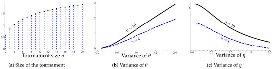
Figure 3.
Comparative statics on the expected ability of tournament winner. The graphs display the expected ability of the tournament winner as a function of the tournament size (a), the variance of ability (b), and the variance of the noise (c). (a,c) takes value 1/2. (a,b) takes value 1/2. In all panels, ability and noise are normally distributed with mean zero.
5. Tournament Design
Having discussed both the effects of tournament size on effort (Section 3) and selection (Section 4), we can now consider how many agents the principal selects to compete in the promotion tournament. In what follows, we refer to ‘optimal tournament size’ as the number of contestants that maximize the principal’s expected utility given agents’ unique equilibrium pure strategies.
When choosing the number of competitors, the principal maximizes her ex ante expected utility, taking into account the effect of tournament size on effort and selection. That is, her maximization problem is
Our first result establishes that tournaments of size 2 are generally suboptimal from the principal’s perspective.
Remark 1.
The optimal tournament size is strictly less than 3 only if .
Proof.
Proofs for this section are collected in Appendix C. □
Note that this result does not require any restriction on (besides the assumption that it is weakly increasing in its arguments) or on the distributions of and . It is a direct consequence of Corollary 1 and Proposition 3. Increasing the size of the tournament from two to three agents has no effect on an agent’s effort. Since the principal always gains in terms of selection, she prefers not to restrict the set of contestants to two unless the cost of adding a third competitor is very large.
This result has important implications when one interprets elections as a tournament. Effort in this case can be understood as campaign spending meant to manipulate the voter’s evaluation of candidates. In this case, is constant in agents’ output. Alternatively, effort may correspond to commitment to targeted spending, with , and as the cost of advertising campaign promises (see Prato & Wolton, 2016). Alternatively, candidates may actually invest in policy quality, with this investment depending on the candidates’ ability and being imperfectly observable by voters (a setting adapted from Hirsch & Shotts, 2015). Finally, stretching the analogy slightly, one could think of effort in a more Downsian fashion. Under this perspective, the principal is the median voter, and effort is the cost of moving away from one’s ideal point (in this mapping we briefly describe, voters need to have linear utility in policy position, whereas candidates have non-linear utility functions). Then, ability can be thought as a common-value valence shock. The policy promises and valence of each candidate need then to be imperfectly observable due to the noise of the campaign (captured by ). Remark 1 indicates that, independently of the interpretation of agents’ output, two-candidate elections are generally inefficient from the electorate’s point of view. It suggests that there may be some welfare gain for voters from encouraging at least one more candidate to participate in elections (as long as the marginal cost of increasing the number of candidates is relatively small).
To provide more details on the optimal tournament size, we return throughout the remainder of this section to the case of normally distributed ability () and luck (). We further impose that the agents’ cost function is quadratic: , with sufficiently small so that the second-order conditions hold. This second assumption allows us to identify the direct effect of size on effort, not the effect mediated through the shape of the cost function.9
We focus on two natural situations. First, we suppose that the principal’s preference for effort depends only on the output of a single agent; that is, . Second, we assume that the principal cares about total effort (equivalently, total output): .
5.1. Optimal Tournament Size When the Principal Cares About Single Effort
This first situation subsumes several distinct objectives that a principal might have. It corresponds to a principal valuing average output (since agents play a symmetric strategy). This naturally occurs when the principal delegates policies to subordinate units and is concerned about all entities receiving similar treatment—either to avoid inconsistencies, as in the case of judicial decisions, or to ensure some common standards, as in the case of education policies. Such an objective is also consistent with the principal seeking to maximize minimum output. In domains where negative spillovers are present (e.g., environmental policy), a principal may want to minimize the damage caused by the worst performer. In the case of antiterrorism policies, a principal wants to strengthen the weakest link (De Mesquita, 2007; Powell, 2007). Finally, the function is also consistent with a principal only taking into account the performance of the promoted agent (or, equivalently, the best performance). Examples of such objectives include elections (as discussed above), maximizing the quality of implemented policies (Hirsch & Shotts, 2015), or innovation.10
Under our conditions on the cost function, there exists a unique size maximizing the principal’s expected welfare, which we denote as . The next proposition describes how varies with the model parameters.
Proposition 5.
When , Equation (10) has a unique maximum with the following properties:
- (i)
- is decreasing with V;
- (ii)
- is increasing with .
Recall that the expected ability of the promoted agent does not depend on the tournament prize V, whereas an agent’s effort is strictly increasing in V. Nonetheless, Proposition 5 indicates that the optimal size is decreasing in the value of promotion. To understand this result, observe that when choosing , the principal compares the marginal gain from increasing the size of the tournament by one agent with the marginal cost. As highlighted in Proposition 2, effort is decreasing with size. Further, since effort is linear in V (under our assumption of quadratic cost of effort), as the value of the prize increases, so does the difference between and (see in Figure 2b how the gap between the marginal benefits of effort for tournament of size 4 and tournament of size 10 increases with V). Therefore, as V increases, it becomes more costly, in terms of reduced effort, to increase the size of the tournament by one agent. Hence, is decreasing in V.
A similar logic explains why the optimal size is increasing in the variance of ability even though tends to depress effort. An increase in variance reduces the loss in effort terms from increasing the size of the tournament (see Figure 2c for an illustration of this reduced difference). Further, greater variance in abilities not only increases the (expected) quality of the promoted agent, but it also enhances the selection gain from adding one agent, as the chance of getting a high-ability agent increases (see Figure 3b, where the distance between the expected ability of the winner of a tournament of size 10 and the expected ability of the winner of a tournament of size 4 is much larger for high than for low ).
5.2. Optimal Tournament Size When the Principal Cares About Total Effort
Situations when the principal values total effort are quite common. For example, a profit-maximizing firm seeks to maximize the performance of its semi-independent divisions competing in different markets. Similarly, an editor wants to increase the quality of reporting among all journalists. Totalitarian leaders aim to maximize the performance of all party members—whether regional heads (Li & Zhou, 2005; Lu & Landy, 2014; Maskin et al., 2000) or rank-and-file members (Montagnes & Wolton, 2019).
The next Lemma establishes that while individual effort is decreasing and convex in n, total effort is increasing and concave in n.
Lemma 1.
Total equilibrium effort is strictly increasing (i.e., ) and strictly concave (i.e., for all ).
We can then use Lemma 1 to establish the properties of the optimal tournament size—denoted as —when the principal cares about total effort.
Proposition 6.
When , Equation (10) has a unique maximum with the following properties:
- (i)
- ;
- (ii)
- is increasing with V;
- (iii)
- is decreasing with .
When the principal cares about individual effort, an increase in tournament size only improves selection. In contrast, when the principal values total effort, increasing the size of the tournament has a positive effect on the effort () and selection () components of her objective function. As a direct consequence, the principal has more incentive to increase the size of the tournament in the latter case, and this is reflected in point (i) of Proposition 6.
Points (ii) and (iii) follow from similar reasoning as for Proposition 5. Observe, however, that since total effort is increasing with n, an increase in V tends to magnify the benefit of adding contestants. Consequently, is increasing with V. The impact of , in turn, is due to its negative impact on effort (which attenuates the positive effect of increasing tournament size) and selection (as higher performances are more likely to be due to luck than ability).
Notice that Proposition 6 says nothing about the effect of an increase in the variance of abilities. This results from the conflicting effects of increased on the marginal benefit of adding a participant. Greater variance in abilities, by depressing effort (Proposition 2), mitigates the gain in total effort, whereas by improving (Proposition 4), it enhances the selection gain.
6. Discussion
Any hierarchical structure presupposes promotion—the selection of the agent(s) most able to perform at the higher level. In turn, promotion generates incentives akin to tournaments. Consequently, tournaments should primarily be understood as a selection mechanism rather than a scheme to promote effort.
Not surprisingly, a large body of work on tournaments in economics has long established that (sufficiently complete) contracts always generate higher output than tournaments (Green & Stokey, 1983; Nalebuff & Stiglitz, 1983; Prendergast, 1999). But this literature misses much of the story. As in elections (Fearon, 1999), effort in promotion-based hierarchies is a by-product of selection incentives, as competing agents attempt to manipulate the principal’s evaluation of their ability.
Because promotions are intrinsically a selection mechanism, the principal cannot commit to any fixed promotion standards other than promoting the agent with the highest expected ability. Any setting that presupposes other promotion rules falls short of Fearon’s (1999) critique.
Agents’ efforts do not matter at the time of promotion, but they do affect the design of the tournament. Importantly, we cannot evaluate the effectiveness of a tournament without a proper understanding of the principal’s objective. When she values total effort, tournaments tend to be large and generate low individual effort. When she values individual effort, tournaments are relatively smaller and generate relatively high effort. When the principal’s objective is unobservable to researchers, the relationship between size and the value of promotion can help to recover it. Indeed, the correlation is positive if the principal values total effort.
We derived our results under additive separability of ability and effort. The qualitative story, however, carries over if output is instead multiplicative, , where each is drawn from the same distribution and remains unknown to the agent when choosing effort. In that setting, a higher realization of still makes effort more valuable, so equilibrium effort again hinges on the probability that an extra unit of effort shifts the promotion ranking. Although the algebra becomes less transparent—agents must reason about the product rather than a simple sum—the central comparative statics insight survives: once the tournament has more than two contestants, the expected output of the leading rival continues to rise with tournament size, preserving the accountability–selection tradeoff highlighted in the paper.
We also assume that the principal can perfectly control the number of tournament participants. This can easily be accomplished by an autocrat (who can include agents and exclude others, without too much concern for participation constraints). This may be more difficult in democratic settings. We believe that democratic leaders have other tools at their disposal to obtain tournaments of optimal size. For example, they can manipulate rewards or costs to participate in a tournament.11 Yet, the prevalence of two-candidate elections (or rather elections with only two viable candidates), despite their inefficiency for voters (Remark 1), suggests that the incentives of those who design tournaments—office-holders—may be distinct from the incentives of the principal within a tournament—the electorate. We leave the analysis of this question for future research.
Author Contributions
Conceptualisation: B.P.M. and J.J.; Formal analysis, B.P.M. and S.W.; Writing: B.P.M. and S.W. All authors have read and agreed to the published version of the manuscript.
Funding
This research received no external funding.
Data Availability Statement
No new data were created or analyzed in this study. Data sharing is not applicable to this article.
Conflicts of Interest
The authors declare no conflicts of interest.
Appendix A. Properties of Agents’ Effort
Throughout the Appendix, we assume that is distributed over (with not necessarily finite). Denote and as the associated standardized (resp.) cumulative distribution function (CDF) and probability density function (pdf). Since and are symmetric and unimodal around 0, and and are independent, is symmetric and unimodal around 0. Consequently, over the relevant domain.
In this section, we establish properties of the agents’ level of effort. In doing so, we prove Propositions 1 and 2.
Proof of Proposition 1.
As explained in the text, agent i’s objective is
Denote as the (symmetric) effort of all other agents. The probability that i is promoted is as follows (recall that indicates the standardized distribution): .
The first order condition is
Imposing symmetry, we obtain that the agent’s effort in the symmetric equilibrium——is implicitly defined by
Accordingly, we concentrate on the symmetric equilibrium derived in Proposition X. Standard arguments imply that this equilibrium is in fact the only one satisfying the usual regularity and stability criteria; we therefore do not reproduce those arguments here.
In what follows, we look at the property of effort in the symmetric equilibrium. Denote the equilibrium effort to be implicitly defined by Equation (A2). To establish Proposition 2, it is useful to denote the equilibrium marginal benefit of effort as follows:
□
Lemma A1.
The marginal benefit of effort is defined as follows:
- 1.
- Linearly increasing in V;
- 2.
- Decreasing and convex in the variance ;
- 3.
- Decreasing and concave in the number of participants n for .
Proof.
The proof of point 1 follows directly from an examination of Equation (A3) and is thus omitted.
Regarding points 2 and 3, first we use a change of indices () to rewrite as
By integrating by parts, we then obtain
For point 2, differentiating then yields
It can then be checked that .
For point 3, denote .12 First, notice that for all ,
Clearly, . Since , or equivalently, , we obtain .
To prove the concavity argument, we use the following claim:
Claim A1.
for all .
Proof.
To prove the claim, define the function for all and . Notice that for all . It is thus sufficient to show that is decreasing in (strictly for some ) to prove the claim.
Since the function is in both arguments for and , we obtain
Observe that . Further,
Observe that and . Notice that since , . This implies that for all . Further, for all and for all . Putting together all the properties of , we obtain that for all , which proves the claim. □
Using the claim, for all and all , we thus have . To complete the proof, notice that
Thus, point 3 holds for all . □
Remark A1.
The marginal benefit of effort is the same in tournaments with two and three participants.
Proof.
See Equation (A7), with . □
Remark A2.
For , effort is constant in the number of players if and only if ϵ is uniformly distributed over .
Proof.
If is uniformly distributed over , then for all and for all n. If does not follow a uniform distribution, then there exists , such as . By Equation (A7), then . □
Proof of Proposition 2.
The proof follows directly from Lemma A1 and the convexity of . □
Proof of Corollary 1.
Observe that (ignoring arguments whenever possible)
Since by Lemma A1 and by assumption, the result holds.
A similar reasoning holds for , noting that .
Finally, we establish some additional properties of the marginal benefit of effort.
Lemma A2.
The marginal benefit of effort satisfies, for all and , the following:
- (i)
- ;
- (ii)
- ;
- (iii)
- ;
- (iv)
- ;
- (v)
- .
Proof.
The proof of point (i) follows directly from Equation (A6) and .
The proof of point (ii) follows directly from examination of Equation (A7) and .
To prove point (iii), observe that by Equation (A7), so .
To prove point (iv), we obtain, using Equation (A5) for ,
Consider for and the function
Observe that for all . We prove by induction that for all and all . For , observe that for all . Suppose that the claim holds for . Denote as the (partial) derivative of with respect to its x. Observe that
where the inequality follows from and (by induction). Given , this implies that for all .
Observe that for all , so by Equation (A9).
For point (iii), notice that for all ,
From Equation (A8), for all . Using the properties of , for all . The claim follows by iterating the inequality. □
Proof of Corollary 2.
This is directly determined from Lemma A2. □
Appendix B. Properties of Tournament Winner
As explained in the text, the principal selects (in the symmetric equilibrium) the agent with the highest performance. Since the principal correctly anticipates all agents’ efforts, this is equivalent to selecting the highest realization of the uncertainty component . Denote . We thus have . Using the standardized pdf and CDF, this is equivalent to (the second equality follows from change of indices). Hence, we have
The expected competence of the tournament winner (using ) is then
Proof of Proposition 3.
To prove the proposition, we just need to show that is increasing with n (since and are positively correlated). Notice that for all , (with strict inequality for all finite ). Hence, strictly first-order stochastically dominates . Hence, for all .
To prove concavity, it is useful to denote . Using Equation (A10),
The third equality follows from integration by parts. This implies that
For all and , . □
Imposing the normal distributions on and , can be expressed as
where the second line uses .
Proof of Proposition 4.
Points 1 and 2 follow from taking the derivative of with respect to and , respectively. □
We now prove some additional properties of selection in tournament. To do so, it is useful to define
Lemma A3.
For all and all , is increasing with and decreasing with .
For all and , is decreasing with and increasing with .
Appendix C. Optimal Tournament Design
Throughout, we use the notation . We provide general conditions for our comparative results to hold before imposing the assumption . Further, we assume that and are normally distributed with respective variances and .
The existence of and is guaranteed by the properties of detailed in the text and the bounded nature of the choice set available to the principal (i.e., ).
Proof of Remark 1.
By Remark A1, effort is the same in tournaments with two or three competitors. When the principal cares about average effort, the marginal gain from increasing the tournament from two to three players is thus . When the principal cares about total effort, the marginal gain from increasing the tournament from two to three players is thus . In both cases, the principal is worse off with a tournament with more than two competitors only if the condition stated in the text of the remark holds (note that the condition is also sufficient for average-effort tournament). □
Proof of Proposition 5.
By Milgrom and Shannon (1994), the solution is increasing (decreasing) in a parameter if the objective function exhibits the single-crossing property which is implied by showing increasing (decreasing) differences in the parameter.
Denote the benefit of increasing the size of a tournament as
Further, let, for ,
The objective function exhibits increasing (decreasing) differences in , , or V whenever is increasing (decreasing) in the variable.
To prove point (i), observe that, using Equations (A6) and (A14), and ,
Imposing the quadratic cost assumption (i.e., ), by Corollary 2 and Proposition 3.14
The proof of points (ii) and (iii) follows from a similar reasoning in noting that does not depend on V. □
Proof of Proposition 6.
The proof again uses the increasing (decreasing) differences property of the objective function. Denote the benefit of a tournament as
Further, let, for ,
To prove point (i), observe that, using Equations (A9) and (A14), and ,
Imposing the quadratic cost assumption (i.e., ), by Lemma A1 and Proposition 3.15
The proof of point (ii) follows from a similar reasoning noting that does not depend on V. □
Appendix D. Tournaments with Proportional Prize Price
In this last Appendix, we study some properties of tournament when the prize increases with the size of the tournament. Throughout, we focus on the case when luck and ability are both normally distributed ( and ). Recall that .
Remark A3.
Consider a proportional prize increase in a tournament, with a prize equal to . As the size of the tournament increases, the effort () of each agent increases.
Proof of Remark A3.
We want to show that effort is increasing in n.
The new equilibrium effort for agent i is defined by
Adapting from Proposition 2, it is sufficient to show that to prove increasing effort. By integration-by-parts, , which yields . We exploit the integration-by-parts technique again, which yields
We can then write the difference in effort between n- and -person tournament as follows:
To see how we reach (A23), notice that in the second equality, we have given the assumption of normal distributions. Also note that for any normal distribution with mean 0 and variance , we have =.
To finish the proof, it is enough to note that the first and second bracketed terms in line (A23) are negative, and so the whole expression is positive as required. □
Remark A4.
There exists such that, for prizes , the ex ante utility of agents is decreasing.
Proof of Remark A4.
Consider the agent’s FOC as
Let , and then the equilibrium effort is
The ex ante total cost for the agent is thus , which follows as
And
If we assume that , then the second order of the total cost function (Equation (A25)) is strictly convex; hence, the total benefit is concave. There would thus exist a beyond which the total benefit starts declining. □
Notes
| 1 | Note that throughout the paper, we use a forward-looking notion of accountability: An institution is more accountable when it gives agents stronger incentives to exert costly effort before outcomes are realized. |
| 2 | In our model, effort is always beneficial for the principal. This does not have to be the case. For example, Hvide and Kristiansen (2003) and Fang and Noe (2022) highlight that tournaments can lead to excessive risk-taking from the principal’s perspective. |
| 3 | This assumption is consistent with evidence on politicians’ skills (albeit in Sweden) collected in Dal Bó et al. (2017). |
| 4 | Our assumption that output is a linear sum of effort, ability, and noise is closest to the model of Lazear and Rosen (1981), but see Nalebuff and Stiglitz (1983) for a model where effort and shocks are not linearly separable. |
| 5 | Equivalently, the principal may care about agent output rather than their effort. This generally does not affect our results (recall agents not considered for promotion produce no output) but only complicates the exposition (see note 10 for more details). We define over and not n so that the function is well defined for all tournament sizes. |
| 6 | Absent this assumption on variances, selection plays a limited role. The competition between agents resembles an all-pay contest with equilibrium supported by mixed strategies over a support that includes zero effort. We implicitly assume that the second-order conditions for the maximization problems are well defined and hold in what follows. |
| 7 | Furthermore, as the proof of Proposition 2 shows, if the single-peaked assumption is reversed and for all , the result is reversed. Assuming the existence of a symmetric equilibrium, effort is increasing with the size of the tournament. |
| 8 | Hence, the null effect of tournament size on effort found in Orrison et al. (2004) is a knife-edge result that relies on their distributional assumption. |
| 9 | See the discussion around Corollary 2. All our results hold as long as for all , with strictly positive but not too large. |
| 10 | If the principal cares about agents’ outputs rather than effort, her objective function becomes , with . In this case, when the principal seeks to maximize the lowest (highest) performance, and the objective function reduces—using the symmetry—to (). All our results remain unchanged for the case of maximizing the best performer and require sufficiently small for the case of maximizing the lowest performer. Focusing on agents’ effort allows us to keep the objective function the same in all three cases described in the text. |
| 11 | An alternative approach would be to vary the degree of centralization in a given state. Greater centralization can be understood as greater tournament. Greater centralization would, however, also increase the value of the prize. Hence, it is different from simply varying the reward of the tournament winner or the cost of participation. |
| 12 | In the text, we consider the slightly different form of differences , where . Considering fixed differences of size k allows for clearer proofs. |
| 13 | To see this, assume that n is a continuous variable (observe that is well defined for n continuous), and note that Equation (A8) is equivalent to , with and . |
| 14 | Observe that the result still holds true as long as for all and is strictly positive. |
| 15 | Observe that the result still holds true as long as for all and is strictly positive. |
References
- Ashworth, S. (2005). Reputational dynamics and political careers. Journal of Law, Economics, and Organization, 21(2), 441–466. [Google Scholar] [CrossRef]
- Ashworth, S. (2012). Electoral accountability: Recent theoretical and empirical work. Annual Review of Political Science, 15, 183–201. [Google Scholar] [CrossRef]
- Cameron, C. M., de Figueiredo, J. M., & Lewis, D. E. (2013). Public sector personnel economics: Wages, promotions, and the competence-control trade-off. National Bureau of Economic Research. [Google Scholar]
- Clark, D. J., & Riis, C. (2001). Rank-order tournaments and selection. Journal of Economics, 73, 167–191. [Google Scholar] [CrossRef]
- Connelly, B. L., Tihanyi, L., Crook, T. R., & Gangloff, K. A. (2014). Tournament theory: Thirty years of contests and competitions. Journal of Management, 40(1), 16–47. [Google Scholar] [CrossRef]
- Dal Bó, E., Finan, F., Folke, O., Persson, T., & Rickne, J. (2017). Who becomes a politician? The Quarterly Journal of Economics, 132(4), 1877–1914. [Google Scholar] [CrossRef]
- De Mesquita, E. B. (2007). Politics and the suboptimal provision of counterterror. International Organization, 61(01), 9–36. [Google Scholar] [CrossRef]
- Eggers, A. C., & Spirling, A. (2016). Party cohesion in Westminster systems: Inducements, replacement and discipline in the house of commons, 1836–1910. British Journal of Political Science, 46(03), 567–589. [Google Scholar] [CrossRef]
- Epstein, L., Knight, J., & Martin, A. D. (2003). The norm of prior judicial experience and its consequences for career diversity on the US Supreme Court. California Law Review, 91, 903–965. [Google Scholar] [CrossRef]
- Fang, D., & Noe, T. (2022). Less competition, more meritocracy? Journal of Labor Economics, 40(3), 669–701. [Google Scholar] [CrossRef]
- Fearon, J. D. (1999). Electoral accountability and the control of politicians: Selecting good types versus sanctioning poor performance. Democracy, Accountability, and Representation, 55, 61. [Google Scholar]
- Fong, C., & McCrain, J. (2024). A tournament theory of congressional committee leadership. Public Choice, 202, 193–215. [Google Scholar] [CrossRef]
- Ghosh, S., & Waldman, M. (2010). Standard promotion practices versus up-or-out contracts. The RAND Journal of Economics, 41(2), 301–325. [Google Scholar] [CrossRef]
- Green, J. R., & Stokey, N. L. (1983). A comparison of tournaments and contracts. The Journal of Political Economy, 91(3), 349–364. [Google Scholar] [CrossRef]
- Groseclose, T., & Stewart, C., III. (1998). The value of committee seats in the House, 1947-91. American Journal of Political Science, 42, 453–474. [Google Scholar] [CrossRef]
- Gürtler, M., & Gürtler, O. (2015). The optimality of heterogeneous tournaments. Journal of Labor Economics, 33(4), 1007–1042. [Google Scholar] [CrossRef]
- Hirsch, A. V., & Shotts, K. W. (2015). Competitive policy development. The American Economic Review, 105(4), 1646–1664. [Google Scholar] [CrossRef]
- Holmström, B. (1999). Managerial incentive problems: A dynamic perspective. The Review of Economic Studies, 66(1), 169–182. [Google Scholar] [CrossRef]
- Höchtl, W., Kerschbamer, R., Stracke, R., & Sunde, U. (n.d.). Incentives vs. selection in promotion tournaments: Can a designer kill two birds with one stone? SSRN Electronic Journal. [Google Scholar] [CrossRef]
- Hvide, H. K., & Kristiansen, E. G. (2003). Risk taking in selection contests. Games and Economic Behavior, 42(1), 172–179. [Google Scholar] [CrossRef]
- Krishna, V., & Morgan, J. (1998). The winner-take-all principle in small tournaments. Advances in Applied Microeconomics, 7, 61–74. [Google Scholar]
- Lazear, E. P., & Rosen, S. (1981). Rank-order tournaments as optimum labor contracts. The Journal of Political Economy, 89(5), 841–864. [Google Scholar] [CrossRef]
- Levy, J., & Zhang, J. (2024). Promotion and demotion contests. Journal of Economic Behavior & Organization, 219, 124–151. [Google Scholar]
- Li, H., & Zhou, L.-A. (2005). Political turnover and economic performance: The incentive role of personnel control in China. Journal of Public Economics, 89(9), 1743–1762. [Google Scholar] [CrossRef]
- Lu, X., & Landy, P. F. (2014). Show me the money: Interjurisdiction political competition and fiscal extraction in China. American Political Science Review, 108, 706–722. [Google Scholar] [CrossRef]
- Malcomson, J. M. (1986). Rank-order contracts for a principal with many agents. The Review of Economic Studies, 53(5), 807–817. [Google Scholar] [CrossRef]
- Maskin, E., Qian, Y., & Xu, C. (2000). Incentives, information, and organizational form. The Review of Economic Studies, 67(2), 359–378. [Google Scholar] [CrossRef]
- Michels, R. (1915). Political parties: A sociological study of the oligarchical tendencies of modern democracy. Hearst’s International Library Company. [Google Scholar]
- Milgrom, P., & Shannon, C. (1994). Monotone comparative statics. Econometrica, 62(1), 157–180. [Google Scholar] [CrossRef]
- Montagnes, B. P., & Wolton, S. (2019). Mass purges: Top-down accountability in autocracy. American Political Science Review, 113(4), 1045–1059. [Google Scholar] [CrossRef]
- Myerson, R. B. (2006). Federalism and incentives for success of democracy. Quarterly Journal of Political Science, 1, 3–23. [Google Scholar] [CrossRef]
- Nalebuff, B. J., & Stiglitz, J. E. (1983). Prizes and incentives: Towards a general theory of compensation and competition. The Bell Journal of Economics, 14, 21–43. [Google Scholar] [CrossRef]
- Orrison, A., Schotter, A., & Weigelt, K. (2004). Multiperson tournaments: An experimental examination. Management Science, 50(2), 268–279. [Google Scholar] [CrossRef]
- Powell, R. (2007). Defending against terrorist attacks with limited resources. American Political Science Review, 101(03), 527–541. [Google Scholar] [CrossRef]
- Prato, C., & Wolton, S. (2016). The voters’ curses: Why we need goldilocks voters. American Journal of Political Science, 60(3), 726–737. [Google Scholar] [CrossRef]
- Prendergast, C. (1999). The provision of incentives in firms. Journal of Economic Literature, 37(1), 7–63. [Google Scholar] [CrossRef]
- Ryvkin, D. (2010). The selection efficiency of tournaments. European Journal of Operational Research, 206(3), 667–675. [Google Scholar] [CrossRef]
- Waldman, M. (2013). Classic promotion tournaments versus market-based tournaments. International Journal of Industrial Organization, 31(3), 198–210. [Google Scholar] [CrossRef]
- Wang, R., Lützenrath, J., & Wolton, S. (2022). Can mass purges root out corruption? SSRN. [Google Scholar] [CrossRef]
Disclaimer/Publisher’s Note: The statements, opinions and data contained in all publications are solely those of the individual author(s) and contributor(s) and not of MDPI and/or the editor(s). MDPI and/or the editor(s) disclaim responsibility for any injury to people or property resulting from any ideas, methods, instructions or products referred to in the content. |
© 2025 by the authors. Licensee MDPI, Basel, Switzerland. This article is an open access article distributed under the terms and conditions of the Creative Commons Attribution (CC BY) license (https://creativecommons.org/licenses/by/4.0/).