The Raiffa–Kalai–Smorodinsky Solution as a Mechanism for Dividing the Uncertain Future Profit of a Partnership

Abstract

Establishing a partnership necessitates agreeing on how to divide future profits or losses. We consider parties who wish to contract on the division of uncertain future profits. We propose to divide profits according to the Raiffa–Kalai–Smorodinsky (K-S) solution, which is the intersection point of the feasible region’s boundary and the line connecting the disagreement and ideal points. It is the only function which satisfies invariance to linear transformations, symmetry, strong Pareto optimality, and monotonicity. We formulate the general problem of designing a contract which divides uncertain future profit between the partners and determines shares of each partner. We first focus on linear and, later, non-linear contracts between two partners, providing analytical and numerical solutions for various special cases in terms of the utility functions of the partners, their beliefs, and the disagreement point. We then generalize the analysis to any number of partners. We also consider a contract which is partially based on the parties’ financial contribution to the partnership, which have a positive impact on profit. Finally, we address asymmetric K-S solutions. K-S solutions are seen to be a useful predictor of the outcome of negotiations, similar to Nash’s bargaining solution.

1. Introduction

A partnership is an arrangement in which several individuals cooperate to advance their mutual interests and share the profits and liabilities of, say, a business venture. In a broad sense, it is any cooperative endeavor undertaken by multiple parties. These parties can be governments, non-profits, businesses, individuals, or a combination. Partnerships are widespread in common law jurisdictions such as the United States, Great Britain, and the Commonwealth, especially in professional service industries. Examples also include a law firm, as well as performers and their managers/agents. If professionals have similar skills (e.g., lawyers, physicians), the motivations of creating a partnership are risk-sharing and economies of scale. If they possess complementary skills, they wish to provide a more complete service.

Parties who are considering creating a partnership need to decide in advance how to divide uncertain future profits (or losses). In some situations, the division may be based on initial investment or number of clients each brings. We shall, however, initially consider partnerships without an initial contribution of resources. This problem was discussed by Wilson (1968) and Levin and Tadelis (2005) in the context of the Nash Bargaining Solution. Recently Gerchak and Khmelnitsky (2019a, 2019b) approached the problem explicitly allowing for different risk attitudes and beliefs, in two different ways. In Gerchak and Khmelnitsky (2019b), somewhat similarly to Wilson (1968), they assumed that one of the partners, who knows the other’s risk attitude and beliefs, proposes a contract to the other, respecting its individual rationality constraint (“Leader-Follower”, LF approach). In Gerchak and Khmelnitsky (2019a), profit was split such that the product of expected utilities (net of expected utilities of disagreement point) was maximized, that is, by the Nash Bargaining Solution (NBS) (Nash, 1953).

The problem of profit sharing in partnerships is studied in various applications in economics, business management, industrial relations, and other fields as it affects incentives, cooperation, risk-sharing, and efficiency of/among the partners. Such applications explore how profit-sharing rules (equal, performance-based, contribution-based, etc.) influence outcomes like business success, partner satisfaction, and fairness perception (see, e.g., Gerchak & Khmelnitsky, 2021). In startups, law firms, consulting firms, medical practices, and joint ventures, how profits are shared can make the difference in the partnership’s outcome.

This article assumes that the profit is split via the Raiffa–Kalai–Smorodinsky (K-S) solution (Gerchak & Khmelnitsky, 2021; Kalai & Smorodinsky, 1975), which is the intersection point of the boundary of the feasible region and a line connecting the disagreement point and the ideal point. The K-S solution is the only function which satisfies the following: invariance to affine transformation, symmetry, strong Pareto optimality, and monotonicity (Kalai & Smorodinsky, 1975). In our setting, the ideal point consists of expected utilities of the entire profit allocated to one partner.

Compared to NBS and other profit-sharing mechanisms, the K-S provides solutions which preserve proportional ratios of gains (rather than maximize product of utility gains as in the NBS approach), resulting in being less sensitive to scaling and risk attitudes issues. The K-S approach avoids outcomes where a stronger party can “crush” the other just because it is better at bargaining; instead, each party’s best-case scenario is respected proportionally. Using the K–S solution can help create agreements that feel fair based on relative expectations often important when long-term cooperation and perceived fairness matter.

Compared to the “Leader–Follower” approach in profit sharing (Gerchak & Khmelnitsky, 2019b), where one party (the leader) moves first, deciding on a profit-sharing rule, contribution level, or other key terms, and the other party (the follower) then reacts optimally to the leader’s choice, the K-S solution does not assume asymmetry in information that leads, as a result, to balanced and fair profit shares for all partners.

After formulating the problem (Section 2), we consider two-partner linear contracts (Section 3), analyzing various special cases. We then extend the analysis to any number of partners (Section 4). Section 5 and Section 6 consider extensions of the two-partner model to cases with non-zero disagreement points and with non-linear contracts, respectively. Section 7 and Section 8 deal with an asymmetric contract formulation and a formulation with profit allocation that is partially based on relative amounts of initial investments. Section 9 then concludes the paper.

2. Problem Formulation

Let X and x denote random profit and profit value, respectively. Suppose one partner receives r(x), if the realized profit is x, the other partner then receives x − r(x). Let $u_1\left(·\right)$ and $u_2\left(·\right)$ be the utility functions of partners 1 and 2, respectively. These von Neumann–Morgenstern utility functions are assumed to be increasing, continuous, concave, and almost differentiable everywhere: $u_i^{\prime }\left(·\right)>0, {u_i}^{″}\left(·\right)\le 0, i=1,2$ (e.g., Muthoo, 1999).

Let ${\phi }_1\left(·\right)$ and ${\phi }_2\left(·\right)$ be the pdfs of the profit, which represent the beliefs of partners 1 and 2, respectively; the two functions are defined over a common support:

$${\phi }_i\left(x\right)>0, i=1,2 \forall x\in \left(x_0, x_1\right).$$

The corresponding cdfs are $F_1\left(·\right)$ and $F_2\left(·\right).$ From its definition, the K-S solution is the point closest to the ideal point $\left(E_1\left(u_1\left(X\right)\right), E_2\left(u_2\left(X\right)\right)\right)$ among all feasible points in the expected utilities domain that lie on the line which connects the ideal point and the disagreement point of the partners denoted here by $\left(d_1, d_2\right).$ We assume that

$$0\le d_1<E_1\left(u_1\left(X\right)\right), 0\le d_2<E_2\left(u_2\left(X\right)\right).$$

The determination of the K-S solution is equivalent to solving the following optimization problem:

$$\underset{r\left(X\right)}{\max }{E}_1\left(u_1\left(r\left(X\right)\right)\right)$$

(1)

s.t.

$${\displaystyle \frac{E_1\left(u_1\left(X\right)\right)-E_1\left(u_1\left(r\left(X\right)\right)\right)}{E_1\left(u_1\left(r\left(X\right)\right)\right)-d_1}}={\displaystyle \frac{E_2\left(u_2\left(X\right)\right)-E_2\left(u_2\left(X-r\left(X\right)\right)\right)}{E_2\left(u_2\left(X-r\left(X\right)\right)\right)-d_2}},$$

(2)

$$0\le {\displaystyle \frac{d}{dx}}r(x)\le 1$$

(3)

We note that (1)–(3) is not a unique statement of the K-S problem. Another equivalent formulation can be obtained by replacing partner 1’s expected utility by partner 2’s expected utility in objective (1). In general, maximizing any non-negative linear combination of the expected utilities of the two partners would give the same solution. In the following sections, we present closed-form solutions to the optimization problem (1)–(3) where possible and turn to numerical approximations in cases where no analytical solution exists.

3. Linear Contracts

We pay particular attention to affine (“linear”) contracts, $r\left(x\right)=px+K$, $0\le p\le 1,$ where K is transferred from the other partner, as most contracts used in practice are linear. Further, the accounting literature primarily employs the LEN model, where the contract is linear (Feltham & Xie, 1994). Typical linear contracts are

$$\left(K,X-K\right), \left(pX,\left(1-p\right)X\right), \left(pX+K,\left(1-p\right)X-K\right), 0\le p\le 1.$$

Assume, for now, that $d_1=d_2=0$. Then, the K-S condition simplifies to

$${\displaystyle \frac{E_1\left(u_1\left(X\right)\right)}{E_1\left(u_1\left(r\left(X\right)\right)\right)}}={\displaystyle \frac{E_2\left(u_2\left(X\right)\right)}{E_2\left(u_2\left(X-r\left(X\right)\right)\right)}}.$$

(4)

Example 1.

Consider risk neutral partners, where $u_1\left(r\right)=u_2\left(r\right)=r$. For a linear contract that satisfies (4), it holds that

$$K={\displaystyle \frac{(1-2p)E_1\left(X\right)E_2\left(X\right)}{E_1\left(X\right)+E_2\left(X\right)}}.$$

(5)

So, $K$ is decreasing in $p$, as one would expect. Also, such a linear contract defines the feasible region in the expected utilities domain:

$$\left(E_1\left(r\left(X\right)\right),E_2\left(X-r\left(X\right)\right)\right)=\left\{\left(u_1,u_2\right)\left|u_2=-u_1\right.+E_2\left(X\right)+p\left(E_1\left(X\right)-E_2\left(X\right)\right)\right\}.$$

(6)

The K-S solution, i.e., the point closest to the ideal point $\left(u_1,u_2\right)=\left(E_1\left(X\right),E_2\left(X\right)\right)$ that satisfies (5) and (6) is as follows:

• For equal means, $E_1\left(X\right)$ = $E_2\left(X\right),$ there are multiple solutions given by

  $$K=\left({\displaystyle \frac{1}{2}}-p\right)E_i\left(X\right),\hspace{1em}0\le p\le 1,\hspace{1em}i=1,2.$$

So, if partner 1’s share is higher than ${\displaystyle \frac{1}{2}}$, it has to make a transfer to the other partner.

Since the problem here is $\underset{p,K}{\mathit{max}}\left[p{E}_1\left(X\right)+K\right]$, s.t. $K={\displaystyle \frac{(1-2p)E_1\left(X\right)E_2\left(X\right)}{E_1\left(X\right)+E_2\left(X\right)}}$, then we actually wish to $\underset{p}{\mathit{max}}\left[p{E}_1\left(X\right)+{\displaystyle \frac{(1-2p)E_1\left(X\right)E_2\left(X\right)}{E_1\left(X\right)+E_2\left(X\right)}}\right]$.

Since the objective is linear in p with the slope of ${\displaystyle \frac{E_1\left(X\right)\left(E_1\left(X\right)-E_2\left(X\right)\right)}{E_1\left(X\right)+E_2\left(X\right)}}$, then

• For $E_1\left(X\right)>E_2\left(X\right),$ the solution is $p=1$ and $K=-{\displaystyle \frac{E_1\left(X\right)E_2\left(X\right)}{E_1\left(X\right)+E_2\left(X\right)}}$; i.e., K is negative. (transfer from P1 to P2).
• For $E_1\left(X\right)<E_2\left(X\right)$, the solution is $p=0$ and $K={\displaystyle \frac{E_1\left(X\right)E_2\left(X\right)}{E_1\left(X\right)+E_2\left(X\right)}}$; i.e., K is positive. (transfer from P2 to P1).

Example 2.

Let $K=0,$ i.e., $r\left(x\right)=px, {\phi }_i\left(x\right)={\lambda }_i{e}^{-{\lambda }_{i}x}, x\ge 0$ and $u_i\left(r\right)=u_i\left(1-e^{-{\mu }_{i}r}\right).$  $i=1,2$ (CARA). Then, the K-S condition reduces to the following quadratic equation:

$$\left({\lambda }_2{\mu }_1-{\lambda }_1{\mu }_2\right)p^2-{\lambda }_1\left({\lambda }_2+{\mu }_2\right)\left(1-2p\right)=0.$$

The unique solution of the latter equation, such that $0\le p\le 1$, is

$$p={\displaystyle \frac{1}{1+\sqrt{\frac{{\lambda }_2\left({\lambda }_1+{\mu }_1\right)}{{\lambda }_1\left({\lambda }_2+{\mu }_2\right)}}}}.$$

It can be shown that p is decreasing in ${\mu }_1$ and increasing in ${\mu }_2$. It is increasing in ${\lambda }_1$ and ${\lambda }_2$ iff ${\displaystyle \frac{{\lambda }_1}{{\lambda }_2}}<{\displaystyle \frac{{\mu }_1}{{\mu }_2}} .$ That is, a partner’s share of profit should increase in their own risk aversion and decrease in the other partner’s risk aversion. It is decreasing in the means of both partners’ subjective distributions if ${\displaystyle \frac{{\lambda }_1}{{\lambda }_2}}<{\displaystyle \frac{{\mu }_1}{{\mu }_2}}$.

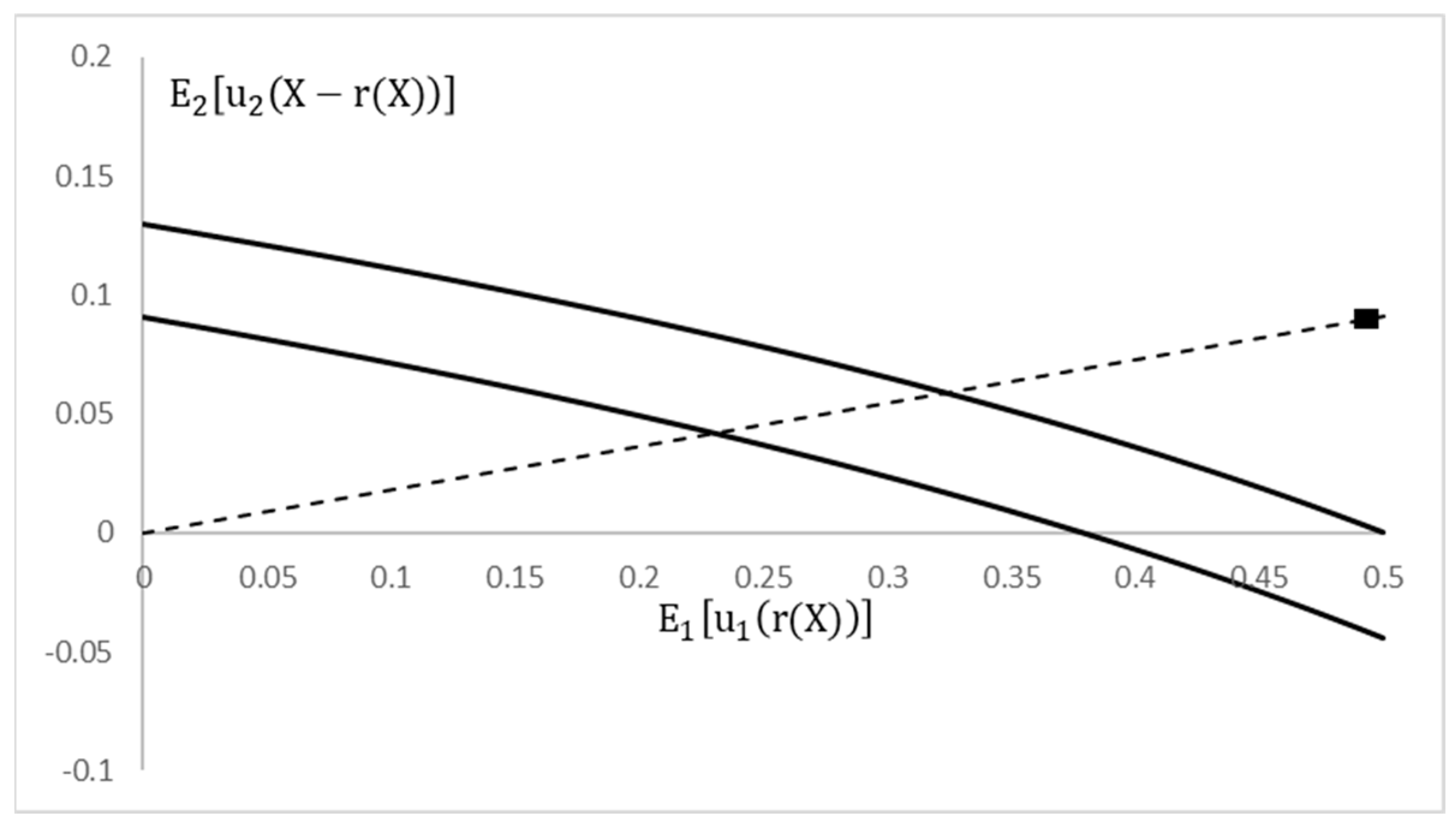
Example 3.

Now Let $r\left(x\right)=px+K, {\phi }_i\left(x\right)={\lambda }_i{e}^{-\lambda ,x}$ and $u_i\left(r\right)=u_i\left(1-e^{-{\mu }_{i}r}\right), i=1, 2.$

Figure 1 presents the feasible region of the expected utilities for the parameters

$$u_1=u_2=1,{ \lambda }_1=1, { \lambda }_2=2, {\mu }_1=1, \hspace{1em}\hspace{1em}{\mu }_2=0.2.$$

The region is bounded from above and below by the lines presenting the contracts with $p=1$ and $p=0$, respectively, where K is free. The dashed line connects the origin with the ideal point shown by the black square and located at (0.5, 0.091). The K-S solution is thus located at the intersection of the dashed line and the upper bound of the feasible region.

An analytic expression for the K-S solution is available for some specific cases. If, for example, ${\mu }_1={\mu }_2\equiv \mu ,$ then the K-S condition results in the following quadratic equation in $e^{K\mu }$:

$${\displaystyle \frac{\mu (u_1-\frac{{\mathrm{e}}^{-K\mu }{\mathsf{\lambda }}_1{u}_1}{{\mathsf{\lambda }}_1+\mu p})u_2}{{\mathsf{\lambda }}_2+\mu }}={\displaystyle \frac{\mu (u_2-\frac{{\mathrm{e}}^{K\mu }{\mathsf{\lambda }}_2{u}_2}{{\mathsf{\lambda }}_2+\mu -\mu p})u_1}{{\mathsf{\lambda }}_1+\mu }},$$

for which the only feasible $K$ is

$$K={\displaystyle \frac{1}{\mu }}ln{\displaystyle \frac{\left({\mathsf{\lambda }}_2-{\mathsf{\lambda }}_1\right)z_1{z}_2+\sqrt{{\left(\left({\mathsf{\lambda }}_1-{\mathsf{\lambda }}_2\right)z_1{z}_2\right)}^2+4{\mathsf{\lambda }}_1{\mathsf{\lambda }}_2\left({\mathsf{\lambda }}_1+\mu \right)\left({\mathsf{\lambda }}_2+\mu \right)z_1{z}_2}}{2{\mathsf{\lambda }}_2({\mathsf{\lambda }}_2+\mu )z_1}},$$

where $z_1={\lambda }_1+\mu p$ and $z_2={\lambda }_2+\mu (1-p)$. Then, after substituting this expression in the objective, $E_1\left(u_1\left(r\left(X\right)\right)\right)$, it is maximized as follows:

• If ${\lambda }_1<{\lambda }_2$ (i.e., $E_1\left(X\right)>E_2\left(X\right)$) and $\mu <{\lambda }_2-{\lambda }_1$, then

  $$p=1 \mathrm{and} K={\displaystyle \frac{1}{\mu }}ln{\displaystyle \frac{{\mathsf{\lambda }}_2-{\mathsf{\lambda }}_1+\sqrt{{\left({\mathsf{\lambda }}_1+{\mathsf{\lambda }}_2\right)}^2+4{\mathsf{\lambda }}_1\mu }}{2\left({\mathsf{\lambda }}_2+\mu \right)}};$$
• If ${\lambda }_2<{\lambda }_1$ and $\mu <{\lambda }_1-{\lambda }_2$, then

  $$p=0 \mathrm{and} K={\displaystyle \frac{1}{\mu }}ln{\displaystyle \frac{{\mathsf{\lambda }}_2-{\mathsf{\lambda }}_1+\sqrt{{\left({\mathsf{\lambda }}_1+{\mathsf{\lambda }}_2\right)}^2+4{\mathsf{\lambda }}_2\mu }}{2{\mathsf{\lambda }}_2}};$$
• Otherwise, if $\mu \ge \left|{\lambda }_1-{\lambda }_2\right|$, then

  $$p={\displaystyle \frac{1}{2}}+{\displaystyle \frac{{\lambda }_2-{\lambda }_1}{2\mu }}$$

  $$K={\displaystyle \frac{1}{\mu }}ln{\displaystyle \frac{\left({\mathsf{\lambda }}_2-{\mathsf{\lambda }}_1\right)z_1{z}_2+\sqrt{{\left(\left({\mathsf{\lambda }}_1-{\mathsf{\lambda }}_2\right)z_1{z}_2\right)}^2+4{\mathsf{\lambda }}_1{\mathsf{\lambda }}_2\left({\mathsf{\lambda }}_1+\mu \right)\left({\mathsf{\lambda }}_2+\mu \right)z_1{z}_2}}{2{\mathsf{\lambda }}_2({\mathsf{\lambda }}_2+\mu )z_1}}.$$

An illustration of this case is shown in Figure 2.

Another case where an analytic solution can be derived is the limit when ${\mu }_1\to 0$ and ${\lambda }_1={\lambda }_2\equiv \lambda$, ${\mu }_2=1$. In such a case, partner 1’s utility tends to be zero regardless of the contract, and the K-S problem is solved by maximizing the expected utility of partner 2. The solution is $p=1$, with a negative K that solves $\lambda ={\displaystyle \frac{e^K}{1-K-e^K}}$. In the opposite limit case, where ${\mu }_2\to 0$ and ${\mu }_1=1$, the K-S contract is $p=0$ with a positive K that solves

$$\mathsf{\lambda }={\displaystyle \frac{e^{-K}}{1+K-e^{-K}}}.$$

Example 4.

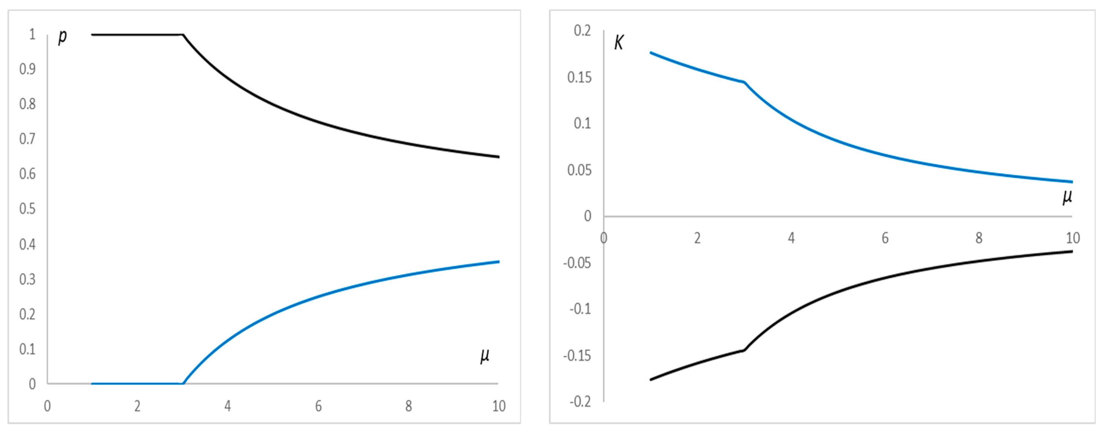
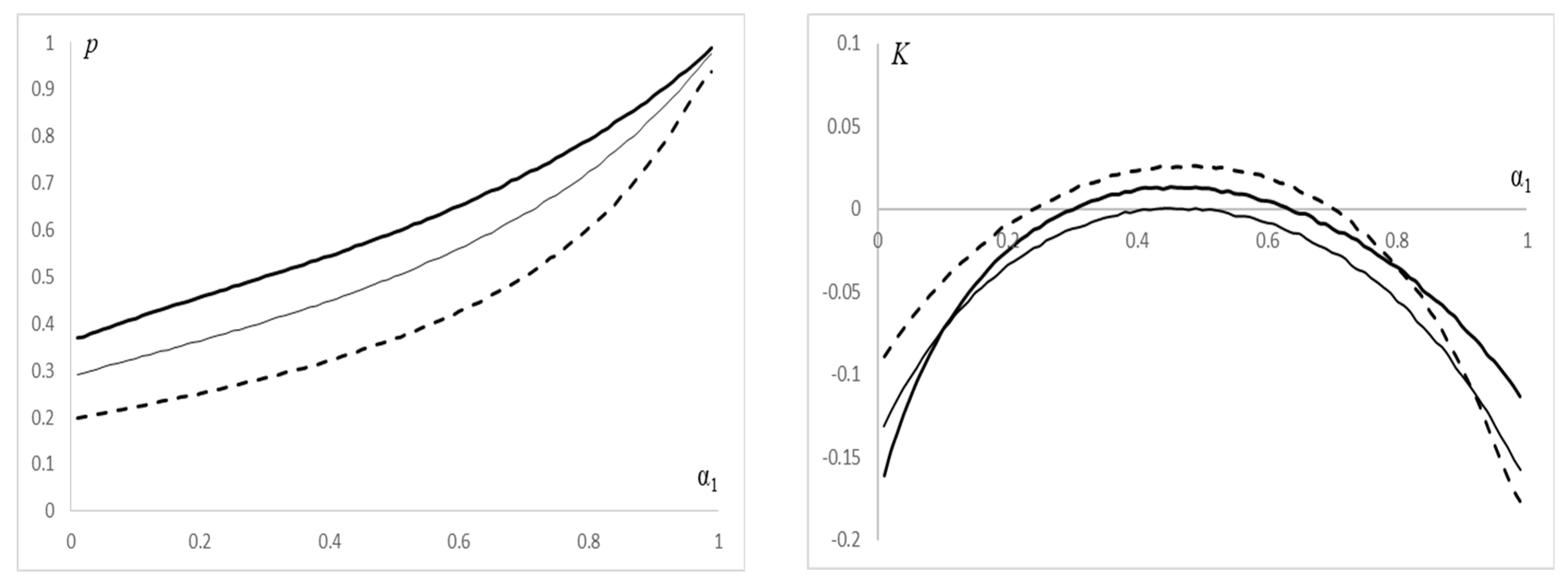
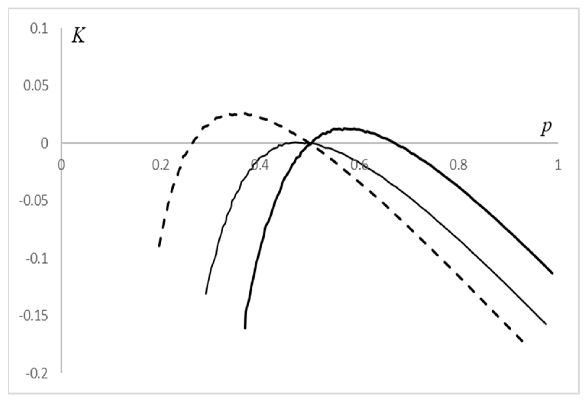
$r\left(x\right)=px+K$, $u_i\left(r\right)={\left(a+r\right)}^{{\alpha }_i}$, $r>-a$, $0<{\alpha }_i<1$, $a\ge 0$, $X_i~U\left[0, 1\right]$, $i=1, 2$. For the utility functions to be properly defined for all $x\ge 0$, the value of K must be in $\left[-a,a\right]$. The K-S condition (4) here is as follows:

$$\begin{array}{l}\left(1-p\right)\left({\left(1+a\right)}^{1+{\alpha }_2}-a^{1+{\alpha }_2}\right)\left({\left(a+K+p\right)}^{1+{\alpha }_1}-{\left(a+K\right)}^{1+{\alpha }_1}\right)\\ \hspace{1em}\hspace{1em}\hspace{1em}\hspace{1em}\hspace{1em}\hspace{1em}=p\left({\left(1+a\right)}^{1+{\alpha }_1}-a^{1+{\alpha }_1}\right)\left({\left(1+a-K-p\right)}^{1+{\alpha }_2}-{\left(a-K\right)}^{1+{\alpha }_2}\right).\end{array}$$

In the limit case where ${\alpha }_1\to 1$ and ${\alpha }_2\to 0$, multiple solutions of the K-S problem satisfy

$$K={\displaystyle \frac{1}{2}}\left(1-p\right), 0\le p\le 1.$$

In the opposite limit case, where ${\alpha }_1\to 0$ and ${\alpha }_2\to 1$, multiple solutions of the K-S problem satisfy

$$K=-{\displaystyle \frac{p}{2}}, 0\le p\le 1.$$

For both cases, solutions are independent of a. For intermediate values of ${\alpha }_1$ and ${\alpha }_2$, a numerical approximation of the unique solution of the K-S problem for $a=2$ is shown in Figure 3 and Figure 4. Figure 3 presents the plots of the two contract parameters, p and K, for ${\alpha }_1\in \left[\mathrm{0,1}\right]$, and Figure 4 presents a parametric plot in the (p,K) domain.

4. Multiple Partners

Assume now that more than two risk-neutral partners consider the linear contract $r_i{=p}_{i}x+K_i$, $i=1,2,\dots ,n$, with

$$p_i\ge 0, {\sum }_{i=1}^n{p}_i=1, {\sum }_{i=1}^n{K}_i=0.$$

(7)

The partners are assumed to be risk-neutral, $u\left(r\right)=r$. We seek the K-S solution, which, according to its definition, is the closest to the ideal point $\left(E_1\left(X\right),\dots , E_n\left(X\right)\right)$ among all feasible points in the expected revenues domain that lie on the line which connects the ideal point and the disagreement point of the partners (in this section $d_i=0, i=1,2,\dots ,n).$ Such a line is presented by the following equations:

$${\displaystyle \frac{E_i\left(X\right)}{E_i\left(p_{i}X+K_i\right)}}={\displaystyle \frac{E_j\left(X\right)}{E_j\left(p_{j}X+K_j\right)}}\forall i,j.$$

(8)

The minimization of the distance to the ideal point subject to constraints (7) and (8) is solved via

$$p_i=\left\{\begin{array}{c}1, if i=i^{*}\\ 0, otherwise\end{array}\right.$$

where $i^{\mathrm{*}}={argmax}_j{E}_j\left(X\right)$, and

$$K_i=\left\{\begin{array}{c}-E_{i^{*}}\left(X\right){\displaystyle \frac{{\sum }_{j=1}^n{E}_j\left(X\right){-E}_{i^{*}}\left(X\right)}{{\sum }_{j=1}^n{E}_j\left(X\right)}}, if i=i^{*}\\ {\displaystyle \frac{E_i\left(X\right)E_{i^{*}}\left(X\right)}{{\sum }_{j=1}^n{E}_j\left(X\right)}}, otherwise.\end{array}\right.$$

The expected profit of partner $i, i\ne i^{*}$

$$J_i={p_i{E}_i\left(X\right)+K}_i={\displaystyle \frac{E_i\left(X\right)E_{i^{\mathrm{*}}}\left(X\right)}{{\sum }_{j=1}^n{E}_j\left(X\right)}},$$

(9)

is proportional to both expected revenues of itself and of the most optimistic partner.

4.1. Partnership vs. Working Alone

We now derive conditions under which conducting business in a partnership with $n-1$ partners has an advantage over conducting business alone. The profit of partner $i$ when working alone is denoted by $Y_i$, and the factor by which the expected profits of the partners grow when working in a partnership of $n$ coworkers is denoted by $g\left(n\right)$. That is,

$$E_i\left(X\right)=g\left(n\right){E(Y}_i), g\left(1\right)=1.$$

We assume that $g\left(n+1\right)\ge g\left(n\right), n\ge 1$, and compare the expected revenue in (9) with ${E(Y}_i)$,

$${\displaystyle \frac{E_i\left(X\right)E_{i^{*}}\left(X\right)}{{\sum }_{j=1}^n{E}_j\left(X\right)}}>{E(Y}_i).$$

By substituting the factor $g\left(n\right)$ in the left-hand side of this inequality, we obtain the following:

$${\displaystyle \frac{g\left(n\right)E\left(Y_i\right)g\left(n\right)E\left(Y_{i^{\mathrm{*}}}\right)}{g\left(n\right){\sum }_{j=1}^{n}E\left(Y_j\right)}}>{E(Y}_i).$$

Equivalently,

$${\displaystyle \frac{g\left(n\right)}{n}}{\displaystyle \frac{{E(Y}_i\left)E\right(Y_{i^{\mathrm{*}}})}{\overline{E\left(Y\right)}}}>{E(Y}_i),$$

where $\overline{E\left(Y\right)}$ is the average expected revenue, $\overline{E\left(Y\right)}={\displaystyle \frac{1}{n}}{\sum }_{j=1}^n{E(Y}_j)$. The last inequality shows that a partnership benefits all partners if ${\displaystyle \frac{g\left(n\right)}{n}}>{\displaystyle \frac{\overline{E\left(Y\right)}}{E\left(Y_{i^{*}}\right)}}$ and is detrimental to all in the opposite case, ${\displaystyle \frac{g\left(n\right)}{n}}<{\displaystyle \frac{\overline{E\left(Y\right)}}{E\left(Y_{i^{*}}\right)}}$.

4.2. Increasing the Partnership

Consider now a scenario, where $n$ partners consider adding a new ${(n+1)}^{th}$ partner. The current expected revenue, ${\displaystyle \frac{g\left(n\right)}{n}}{\displaystyle \frac{{E(Y}_i\left)E\right(Y_{i^{*}})}{\overline{E\left(Y\right)}}}$, needs to be compared to the new one, ${\displaystyle \frac{g\left(n+1\right)}{n}}{\displaystyle \frac{{E(Y}_i\left)E\right(Y_{i^{*}})}{E\left(Y_{n+1}\right)/n+\overline{E\left(Y\right)}}}$, $i=1,2,\dots ,n.$ Consider first the case where the addition of the new partner does not alter the identity of the most profitable one, $i^{*}$, i.e., that $E\left(Y_{n+1}\right)$ is not the highest expected revenue in the group. Then, the inclusion of the new partner benefits all (including themself) if

$$E(Y_{n+1})<{\displaystyle \frac{g\left(n+1\right)-g\left(n\right)}{g\left(n\right)/n}}\overline{E\left(Y\right)}.$$

If the new partner is more profitable when working alone than any other partner, then the inclusion of such a partner benefits all (including themself) if

$$E(Y_{n+1})>{\displaystyle \frac{E\left(Y_{i^{\mathrm{*}}}\right)g\left(n\right)}{g\left(n+1\right)-\frac{g\left(n\right)}{n}\frac{E\left(Y_{i^{\mathrm{*}}}\right)}{\overline{E\left(Y\right)}}}}.$$

We note that the two cases above act in opposite directions. The less profitable the new partner in the first case or the more profitable the new partner in the second case, the more the inclusion of such a partner benefits all.

5. Non-Zero Disagreement Points

Assume that there are two partners and, without loss of generality, that $d_1>d_2$ and $E_i\left(X\right)>d_i, i=1,2.$ The K-S condition is as follows:

$${\displaystyle \frac{E_1\left(u_1\left(X\right)\right)-E_1\left(u_1\left(pX+K\right)\right)}{E_1\left(u_1\left(pX+K\right)\right)-d_1}}={\displaystyle \frac{E_2\left(u_2\left(X\right)\right)-E_2\left(u_2\left(X-pX-K\right)\right)}{E_2\left(u_2\left(X-pX-K\right)\right)-d_2}}.$$

(10)

For risk neutral partners, $u_1\left(r\right)=u_2\left(r\right)=r$, we have the following:

$${\displaystyle \frac{E_1\left(X\right)-E_1\left(pX+K\right)}{E_1\left(pX+K\right)-d_1}}={\displaystyle \frac{E_2\left(X\right)-E_2\left(X-pX-K\right)}{E_2\left(X-pX-K\right)-d_2}}.$$

That is,

$$\left((1-p)E_1\left(X\right)-K\right)\left(\left(1-p\right)E_2\left(X\right)-K-d_2\right)=\left(p{E}_2\left(X\right)+K\right)\left(p{E}_1\left(X\right)+K-d_1\right),$$

so,

$$\left(1-2p\right)E_1\left(X\right)E_2\left(X\right)-K\left(E_1\left(X\right)+E_2\left(X\right)-d_2\right)-d_2\left(1-p\right)E_1\left(X\right)=-d_1(K+p{E}_2\left(X\right)).$$

(11)

Thus,

$$K={\displaystyle \frac{\left(1-2p\right)E_1\left(X\right)E_2\left(X\right)-d_2\left(1-p\right)E_1\left(X\right)+d_{1}p{E}_2\left(X\right)}{E_1\left(X\right)+E_2\left(X\right)-d_2-d_1}}.$$

(12)

The K-S solution, i.e., the point closest to the ideal point $\left(u_1,u_2\right)=\left(E_1\left(X\right),E_2\left(X\right)\right)$ that satisfies (12), is as follows:

• For equal means, $E_1\left(X\right)=E_2\left(X\right)$, multiple solutions satisfy

  $$K=\left({\displaystyle \frac{E_i\left(X\right)-d_2}{2E_i\left(X\right)-d_1-d_2}}-p\right)E_i(X), 0\le p\le 1, i=1,2.$$
• If $E_1\left(X\right)>E_2\left(X\right)$, the solution is $p=1$ and $K=-{\displaystyle \frac{E_2\left(X\right)(E_1\left(X\right)-d_1)}{E_1\left(X\right)+E_2\left(X\right)-d_1-d_2}}$;
  i.e., K is negative.
• If $E_1\left(X\right)<E_2\left(X\right)$, the solution is $p=1$ and $K={\displaystyle \frac{E_1\left(X\right)(E_2\left(X\right)-d_2)}{E_1\left(X\right)+E_2\left(X\right)-d_1-d_2}}$;
  i.e., K is positive.

The dependence of K on $E_1\left(X\right)$ and $E_2\left(X\right)$ is further demonstrated by the following derivatives:

$${\displaystyle \frac{dK}{d{E}_1\left(X\right)}}=-{\displaystyle \frac{E_2\left(X\right)-d_2}{{\left(E_1\left(X\right)+E_2\left(X\right)-d_1-d_2\right)}^2}}\left\{\begin{array}{c}{E}_2\left(X\right), if E_1\left(X\right)>E_2\left(X\right)\\ d_1+d_2-E_2\left(X\right), if E_1\left(X\right)<E_2\left(X\right) \end{array}\right.$$

$${\displaystyle \frac{dK}{d{E}_2\left(X\right)}}={\displaystyle \frac{E_1\left(X\right)-d_1}{{\left(E_1\left(X\right)+E_2\left(X\right)-d_1-d_2\right)}^2}}\left\{\begin{array}{c}{d}_1+d_2-E_1\left(X\right), if E_1\left(X\right)>E_2\left(X\right)\\ E_1\left(X\right), if E_1\left(X\right)<E_2\left(X\right) \end{array}\right.$$

In a particular case where $d_1=d_2\equiv d$, the dependence of K on d is given by

$${\displaystyle \frac{dK}{dd}}=-{\displaystyle \frac{{E_1\left(X\right)-E}_2\left(X\right)}{{\left(E_1\left(X\right)+E_2\left(X\right)-2d\right)}^2}}\left\{\begin{array}{c}{E}_2\left(X\right), if E_1\left(X\right)>E_2\left(X\right)\\ E_1\left(X\right), if E_1\left(X\right)<E_2\left(X\right) \end{array}\right.$$

which is negative in the first case and positive in the second.

6. Non-Linear Contracts

Consider two risk-neutral partners and a non-linear contract:

$$r\left(x\right)=K+pf\left(x\right),$$

where $f\left(x\right)$ is positive and increasing. For the zero-disagreement point, the K-S condition satisfies

$$\left(K+p{E}_1\left(f\left(X\right)\right)\right)E_2\left(X\right)+\left(K+p{E}_2\left(f\left(X\right)\right)\right)E_1\left(X\right)=E_1\left(X\right)E_2\left(X\right).$$

Equivalently,

$$K={\displaystyle \frac{E_1\left(X\right)E_2\left(X\right)}{E_1\left(X\right)+E_2\left(X\right)}}-p{\displaystyle \frac{E_1\left(f\left(X\right)\right)E_2\left(X\right)+E_2\left(f\left(X\right)\right)E_1\left(X\right)}{E_1\left(X\right)+E_2\left(X\right)}}.$$

(13)

We see that, again, K decreases in p. Constraint (3) takes the following form:

$$0\le p\le \underset{x_0\le x\le x_1}{\min }{\left[f^{\prime }\left(x\right)\right]}^{-1}.$$

(14)

The K-S solution maximizes the linear objective:

$$\underset{K,p}{\max }\left(K+p{E}_1\left(f\left(X\right)\right)\right),$$

subject to the linear constraints (13) and (14). The solutions are as follows:

If $E_1\left(f\left(X\right)\right)>E_2\left(f\left(X\right)\right)$, then $p=\underset{x_0\le x\le x_1}{\min }{\left[f^{\prime }\left(x\right)\right]}^{-1}$;

If $E_1\left(f\left(X\right)\right)<E_2\left(f\left(X\right)\right)$, then $p=0$;

If $E_1\left(f\left(X\right)\right)=E_2\left(f\left(X\right)\right)$, then any feasible solution solves the problem.

Example 5.

$r\left(x\right)=K+p{x}^a$, ${\phi }_i\left(x\right)=b_i{x}^{b_i-1}$, $0\le x\le 1$, $b_i\ge 1$, $a\ge 1$.

$E_i\left(X\right)={\displaystyle \frac{b_i}{b_i+1}}$, $E_i\left(X^a\right)={\displaystyle \frac{b_i}{b_i+a}}$. Here, $0\le p\le 1/a$ and

$$K=b_1{b}_2{\displaystyle \frac{1-p\left(\frac{b_1+1}{b_1+a}+\frac{b_2+1}{b_2+a}\right)}{b_1\left(b_2+1\right)+b_2\left(b_1+1\right)}}.$$

K increases in a; i.e., the more convex r(x) is, the higher the transfer to that partner.

The rest of the K-S solution is

If $b_1>b_2$, then $p={\displaystyle \frac{1}{a}}$;

If $b_1<b_2$, then $p=0$;

If $b_1=b_2$, then multiple solutions are given by $0\le p\le {\displaystyle \frac{1}{a}}$.

Example 6.

$r\left(x\right)=K+p{e}^x$, $X_i~U[a_i, b_i]$

$E_i\left(X\right)={\displaystyle \frac{a_i+b_i}{2}}$, $E_i\left(e^X\right)={\displaystyle \frac{e^{b_i}-e^{a_i}}{b_i-a_i}}$. Here, p is bounded by $0\le p\le e^{-max\{b_1,b_2\}}$.

The K-S solution is

If ${\displaystyle \frac{e^{b_1}-e^{a_1}}{b_1-a_1}}>{\displaystyle \frac{e^{b_2}-e^{a_2}}{b_2-a_2}}$, then $p=e^{-max\{b_1,b_2\}}$;

If ${\displaystyle \frac{e^{b_1}-e^{a_1}}{b_1-a_1}}={\displaystyle \frac{e^{b_2}-e^{a_2}}{b_2-a_2}}$, then multiple solutions are given by $0\le p\le e^{-max\{b_1,b_2\}}$

for these two cases:

$$K={\displaystyle \frac{\left(a_1+b_1\right)\left(a_2+b_2\right)}{2\left(a_1+b_1+a_2+b_2\right)}}-{\displaystyle \frac{p}{a_1+b_1+a_2+b_2}}\left({\displaystyle \frac{e^{b_1}-e^{a_1}}{b_1-a_1}}\left(a_2+b_2\right)+{\displaystyle \frac{e^{b_2}-e^{a_2}}{b_2-a_2}}\left(a_1+b_1\right)\right).$$

If ${\displaystyle \frac{e^{b_1}-e^{a_1}}{b_1-a_1}}<{\displaystyle \frac{e^{b_2}-e^{a_2}}{b_2-a_2}}$, then $p=0$ and $K={\displaystyle \frac{\left(a_1+b_1\right)\left(a_2+b_2\right)}{2\left(a_1+b_1+a_2+b_2\right)}}$.

7. Asymmetric K-S Solution

This section considers asymmetric K-S solutions (Dubra, 2001; Karos et al., 2018). In our notation, and assuming that $d_1=d_2=0$, an asymmetric solution satisfies

$$E_2\left(u_2\left(X-r\left(X\right)\right)\right)=\lambda E_1\left(u_1\left(r\left(X\right)\right)\right){\displaystyle \frac{E_2\left(u_2\left(X\right)\right)}{E_1\left(u_1\left(X\right)\right)}},$$

(15)

“allowing” $\lambda$ to take any value in $[0,\infty )$. The rationale for such model, and its consequences, are given by Dubra.

Similarly to Section 2, The K-S solution is obtained by solving the following optimization problem:

$$\underset{r(·)}{\max }{E}_1\left(u_1\left(r\left(X\right)\right)\right)$$

(16)

s.t.

$$E_2\left(u_2\left(X-r\left(X\right)\right)\right)=\lambda E_1\left(u_1\left(r\left(X\right)\right)\right){\displaystyle \frac{E_2\left(u_2\left(X\right)\right)}{E_1\left(u_1\left(X\right)\right)}},$$

(17)

$$0\le {\displaystyle \frac{d}{dx}}r\left(x\right)\le 1.$$

(18)

The solutions of (16)–(18) for risk-neutral partners and a linear contract,

$r\left(x\right)=px+K$, are as follows:

• For equal means, $E_1\left(X\right)=E_2\left(X\right)\equiv E\left(X\right)$; multiple solutions are given by

  $$K=\left({\displaystyle \frac{1}{1+\lambda }}-p\right)E\left(X\right), 0\le p\le 1 \downarrow p.$$

  $${\displaystyle \frac{dK}{d\lambda }}=-{\displaystyle \frac{E\left(X\right)}{{\left(1+\lambda \right)}^2}}<0.$$
  So, $K$ is decreasing in $\lambda$ but less so as $\lambda$ grows.
• For $E_1\left(X\right)>E_2\left(X\right)$, the solution is $p=1$ and $K=-\lambda {\displaystyle \frac{E_1\left(X\right)E_2\left(X\right)}{E_1\left(X\right)+\lambda E_1\left(X\right)}}$;
  i.e., K is negative and more so the larger $\lambda$.
• For $E_1\left(X\right)<E_2\left(X\right)$, the solution is $p=0$ and $K={\displaystyle \frac{E_1\left(X\right)E_2\left(X\right)}{E_1\left(X\right)+\lambda E_2\left(X\right)}}$;
  i.e., K is positive and decreasing in $\lambda$.

Example 7.

$r\left(x\right)=px+K$, $u_i\left(r\right)={(a+r)}^{{\alpha }_i}$, $r>-a$, $0<{\alpha }_i<1$, $a\ge 0$,

$X_i~U\left[\mathrm{0,1}\right], i=1,2$. For the utility functions to be properly defined for all $0\le x\le 1$, the value of K must be in $\left[-a, a\right].$ The asymmetric K-S condition (15) becomes

$$\begin{gathered} \lambda \left(1-p\right)\left({\left(1+a\right)}^{1+{\alpha }_2}-a^{1+{\alpha }_2}\right)\left({\left(a+K+p\right)}^{1+{\alpha }_1}-{\left(a+K\right)}^{1+{\alpha }_1}\right) \\ =p\left({\left(1+a\right)}^{1+{\alpha }_1}-a^{1+{\alpha }_1}\right)\left({\left(1+a-K-p\right)}^{1+{\alpha }_2}-{\left(a-K\right)}^{1+{\alpha }_2}\right). \end{gathered}$$

(19)

Objective (16) is increasing in $K$, so $K^{*}=a \Rightarrow p^{*}={\displaystyle \frac{4\lambda a-1}{\lambda +1}}$.

A different kind of a generalization of K-S solution for $d_1=d_2=0$ is as follows:

$$E_2\left(u_2\left(X-r\left(X\right)\right)\right)=E_1\left(u_1\left(r\left(X\right)\right)\right){\left({\displaystyle \frac{E_2\left(u_2\left(X\right)\right)}{E_1\left(u_1\left(X\right)\right)}}\right)}^{\theta }, \theta >0.$$

For a rational and consequences of such model see (Karos et al., 2018). For risk-neutral partners and a linear contract, that equation, which is now

$$E_2\left(\left(1-p\right)X-K\right)=E_1\left(pX+K\right){\left({\displaystyle \frac{E_2\left(X\right)}{E_1\left(X\right)}}\right)}^{\theta },$$

is satisfied for

$$K={\displaystyle \frac{\left(1-p\right)E_2\left(X\right)-p{E}_1\left(X\right)m_{\theta }}{1+m_{\theta }}}, \mathrm{where} {m_{\theta }\equiv \left({\displaystyle \frac{E_2\left(X\right)}{E_1\left(X\right)}}\right)}^{\theta }.$$

Substituting into the objective, which is now

$$\underset{p}{\max }{\displaystyle \frac{p{E}_1\left(X\right)+\left(1-p\right)E_2\left(X\right)}{1+m_{\theta }}},$$

the conclusion is same as for the basic K-S solution: if $E_1\left(X\right)>E_2\left(X\right)$, then $p=1$; if $E_1\left(X\right)<E_2\left(X\right)$, then $p=0$.

8. Division Partly Proportional to Relative Investments

Suppose now that the parties invest $B_i \mathrm{e}\mathrm{a}\mathrm{c}\mathrm{h},i=1,2$, and the profit grows in the magnitude of $B_1+B_2.$ We shall assume that ${profit}_i=X_i+h_i\left(B_1+B_2\right)$, when $X_i$ is, according to partner $i$, the random profit when $B_1+B_2=0,$ and $h_i$ is increasing and functions concavely (reflecting diminishing returns of total investment) with $h_i\left(0\right)=0, i=1, 2.$ Thus, $E\left({profit}_i\right)=E\left(X_i\right)+h_i\left(B_1+B_2\right)\equiv {\tilde{E}}_i$.

Profit sharing is, according to $r\left(x\right)={\displaystyle \frac{B_1}{B_1{+B}_2}}x+K$, based on the fraction of total investment due to one partner. Suppose that $d_i=B_i, i=1, 2,$ thus, in case of disagreement, the parties retain their investments. Then, if parties are risk-neutral, the K-S condition implies that

$$K={\displaystyle \frac{B_2{\tilde{E}}_1({\tilde{E}}_2-B_2)-B_1{\tilde{E}}_2({\tilde{E}}_1-B_1)}{(B_1{+B}_2)({\tilde{E}}_1-B_1+{\tilde{E}}_2-B_2)}}.$$

Note that if $B_i=0$ then ${\displaystyle \frac{dK}{d{B}_j}}<0$.

Special cases:

• Equal investments, $B_1{=B}_2\equiv B.$ Then
  $K={\displaystyle \frac{B\left(E_2-E_1\right)}{2\left(E_1+E_2-2B\right)}},\begin{array}{c}{E}_1<E_2, { E}_1+E_2>2B \mathrm{o}\mathrm{r}\\ E_1>E_2, { E}_1+E_2<2B \end{array}$ $\Rightarrow K\uparrow B,$ in both cases.
• Equal expected profits, $E_1=E_2\equiv E$, and $h_1=h_2\equiv h$. Let $B_2>B_1.$

  $$K={\displaystyle \frac{(B_2-B_1)(E^2+2Eh+h^2-E{B}_1-h{B}_1)}{(B_1{+B}_2)(2E+2h-B_1-B_2)}}={\displaystyle \frac{(B_2-B_1)({\tilde{E}}^2-B_1\tilde{E})}{(B_1+B_2)(2\tilde{E}-B_1-B_2)}}.$$

  $${\displaystyle \frac{dK}{d\tilde{E}}}={\displaystyle \frac{2{\tilde{E}}^2-2(B_1{+B}_2)\tilde{E}+B_1(B_1{+B}_2)}{{(2\tilde{E}-B_1{-B}_2)}^2}}<0\mathrm{if} {\displaystyle \frac{B_1{+B}_2-\sqrt{B_2^2-B_1^2}}{2}}<\tilde{E}<{\displaystyle \frac{B_1{+B}_2+\sqrt{B_2^2-B_1^2}}{2}}.$$

  $${\displaystyle \frac{dK}{d{B}_1}}={\displaystyle \frac{2\tilde{E}(1-2\tilde{E})B_1^3+\tilde{E}(1{+B}_2+4{\tilde{E}}^2)B_1^2+2\tilde{E}(-\tilde{E}+B_2-B_2\tilde{E}+2B_2^2\tilde{E})B_1+\tilde{E}{B}_2^3+\tilde{E}(-4{\tilde{E}}^2-2\tilde{E}+1)B_2^2-2{\tilde{E}}^2{B}_2}{{(B_1{+B}_2)}^2{(2\tilde{E}-B_1{-B}_2)}^2}}$$

The denominator is clearly positive. As for the numerator, some cases are as follows:

$$B_2{=B}_1=1\Rightarrow {\displaystyle \frac{dK}{d\tilde{E}}}>0 \mathrm{i}\mathrm{f}\mathrm{f} \tilde{E}<1$$

$$B_2=2,B_1=1\Rightarrow {\displaystyle \frac{dK}{d\tilde{E}}}>0 \mathrm{i}\mathrm{f} \tilde{E}<{\displaystyle \frac{-1+\sqrt{29}}{4}}~1.07.$$

9. Concluding Remarks

The prediction of negotiation’s outcome via the K-S solution has some attractive properties when used in Operations Management (see Feng et al., 2022), and, as we saw, it can be used for the purpose of this paper as well. We formulated the general K-S profit division problem and showed its consequences for some sharing functions, utility functions and beliefs. Further, we showed that “richer” asymmetric versions (due to Dubra, 2001; Karos et al., 2018) can be used as well. We then focused on the commonly used linear contracts. The disagreement point was shown to have a major impact on the solution.

We also considered a scenario where profit is increasing in partners’ investments, and its shares equal the relative investment in the partnership. Future research in that direction may address diminishing returns on investment, of the type ${\left({\displaystyle \frac{B_1}{{B_1+B}_2}}\right)}^{\alpha }, 0<\alpha \le 1$, and/or profit multiplicative in investments.

One might explore profit sharing when partners generate their own revenue, as well as joint revenue. Cost allocation according to revenues of facility-sharing “partners” could also be of interest.