Abstract
This paper experimentally investigates the relationship between an investor and a project manager. Project managers choose from a pool of projects, the success probabilities of which are uncertain. Investors can change projects, but also have to change project managers if they want to do so. An additional joint project or a voluntary money transfer precedes their interaction. We hypothesize that investors favor projects of managers with whom they share positive experiences at that stage, even though these experiences do not provide any information about the subsequent project’s success probability. Interaction through a voluntary transfer plays a clear and significant role in the investors’ decision-making via bonding, whereas the influence of merely sharing a positive or negative experience proves more complex.
JEL Classification:
D01; D91; G00; G41; M12; M51
1. Introduction
Relationships matter. This statement appears to be true not only for everyday human interaction but also when it comes to business. The experiment presented here is designed to shed further light on the role of (affective) relationships in one specific context: the interaction between an investor and a project manager, who can either be retained or replaced by a new project manager following different experiences shared with that manager, in particular the transfer of a small gift by the manager.
Gifts are a ubiquitous phenomenon, and substantial evidence exists showing that even small gifts may matter for the behavior of the receiver. Evidence comes from various research fields, like social life (Mauss, 1990; Chan & Mogilner, 2017; Chao & Fischer, 2022), politics (Abbink, 2004; Finan & Schechter, 2012; Leight et al., 2020), and economics (Wazana, 2000; Fehr et al., 2009).1 Regarding investment—the focus of this paper—most attention concerns the experimental study of gift exchange using trust or investment games (Berg et al., 1995; for a review, see Johnson & Mislin, 2011). In these games, an investor can transfer money to a recipient who, in turn, can transfer back any share of the proceeds of the investment. Attention typically focuses on the question of how the behavior of the borrower can be controlled or predicted by the lender. In contrast to the one-shot experiments often used to avoid complicating repeated game effects, longer-term personal relationships between investors (lenders) and borrowers form another prominent research area regarding investment. Relationship banking is an important topic in microeconomics and finance (Boot, 2000) and has attracted attention in experimental economics (Cochard et al., 2004; Brown & Zehnder, 2007; Cornée et al., 2012; Cornée & Masclet, 2022). Also in this field, the focus is often on strategic aspects that come into play once an investor-borrower relationship extends through time, like reputation and regulation (Lunawat, 2013; Cornée & Masclet, 2022). Some empirical studies, however, emphasize a link between connectedness and more affective favoritism, where social proximity, relationship intensity, and physical contact play a role (Haselmann et al., 2018; Gabbi et al., 2020; Rehbein & Rother, 2024). More pertinent to this paper, a few studies suggest that connectedness and favoritism may also matter in relationships with managers, specifically regarding the allocation of capital through internal capital markets and managerial appointments (Kuhnen, 2009; Duchin & Sosyura, 2013).
All of these studies are concerned with existing relationships. This paper, in contrast, focuses on the development of an affective relationship between an investor and a project manager through the latter’s transfer of a small gift and its subsequent consequences, particularly relative to the shared experience of a project outcome.
Although a small gift can have a substantial influence on economic decision making, this phenomenon appears to be hard to explain, not only from a standard economic point of view—assuming a rational and selfish “homo economicus”—but also from a non-standard theoretical viewpoint. This is carefully and clearly shown by Malmendier and Schmidt (2017), the experimental study that is most closely related to ours. Their experiment focuses on a decision maker (with a fixed payoff) who has to choose, in the best interest of a client, between two possible projects (50/50 lotteries). Before this choice is made, one of the two producers can send a small gift. Carefully avoiding potential informational and incentive confounds, they find that decision makers strongly respond to gifts, even though they perfectly understand the gift giver’s (self-reported selfish intention. In trying to explain their findings they question the prominent existing models of social preferences relating other-regarding behavior to altruism (Andreoni & Miller, 2002), maximin preferences (Charness & Rabin, 2002), inequality aversion (Fehr & Schmidt, 1999; Bolton & Ockenfels, 2000), type-based reciprocity (Levine, 1998) or intention-based reciprocity (Rabin, 1993; Dufwenberg & Kirchsteiger, 2004): “Our evidence suggests that a gift triggers an obligation to repay, independently of the intentions of the gift giver and the distributional consequences. It seems to create a bond between gift giver and recipient, in line with a large anthropological and sociological literature on gifts creating an obligation to reciprocate.” (Malmendier & Schmidt, 2017, p. 495).2 To capture their findings, they propose a simple extension of the standard (selfish) utility model, where decision maker i attaches a weight to the payoff of counterpart j dependent on the difference between j’s intendedly chosen action affecting i and the action expected by i. Incorporating the expected behavior is seen as the key innovation relative to action-based reciprocity models, where the expectation may be related to past experience (Malmendier & Schmidt, 2017, p. 514).
Interestingly, Pan and Xiao (2016) provide experimental evidence suggesting that it may not be the intended action (which they label as the “pure intention”) that produces this weight but the gift that is actually received (labeled the “received intention”). In fact, from a psychological perspective, it may be questioned whether an intention is even required for an actual gift to be influential (for experimental evidence, see Strassmair, 2009). According to Zhang and Epley (2012) evidence shows that the importance of “It’s the thought that counts” is exaggerated for receivers in gift exchange: “mental state inference, or theory of mind reasoning, is not automatic or even primary in social judgments, but instead must be activated by the social context” (Zhang & Epley, 2012, p. 678). Considering another’s thought requires a trigger for (effortful) motivation and deliberation.
In this respect, the social ties model of van Dijk and van Winden (1997)—that both Malmendier and Schmidt (2017) and Pan and Xiao (2016) refer to—and especially its more recent elaboration: the Affective Ties Model (Bault et al., 2017; van Winden, 2023), seems to provide an interesting alternative for explaining the observed gift effect. This model—ATM for short—concerns the evolutionarily old and automatic emotional appraisal circuitry of the brain rather than the more recently developed deliberation and planning circuitry that the prominent extant reciprocity models are particularly concerned with. The key to ATM is the following two modules (van Winden, 2023). First, an agent-type (friend or foe) appraisal based on the experienced (beneficial or harmful) action of an interaction partner. A deviation of this action from a reference point—called an impulse—triggers an emotion. The valence and intensity of this emotion provide an appraisal of the agent’s type, represented by the value of a parameter α (or its update if a prior exists). Second, and crucial for bonding and an intrinsic motivation for caring, this type of appraisal generates a weight (equal to α)—coined the tie-value—which is attached to the utility of the relevant agent, thereby extending the utility function (as in the Malmendier and Schmidt model referred to above). ATM can be straightforwardly incorporated into a more general behavioral model for accommodating forward-looking and strategic behavior, because it only deals with the weight attached to another agent’s utility.3
Although providing an interesting formal modeling angle on the gift effect, which also predicts a negative effect from a gift that is smaller than expected,4 the Malmendier and Schmidt experiment addresses a very specific context, to wit: a decision maker (DM) asked to behave in the interest of a client, where the client has no choice regarding the DM and the DM faces a single choice between two producers (lotteries), only one of which can send a gift. In this experimental paper, we want to relax these assumptions and move one organizational tier up by focusing on the client (investor, from now on). The investor first randomly selects a DM (manager, from now on) from an anonymous pool. That manager, in turn, can send a gift (monetary transfer) to the investor before randomly selecting and implementing a project (lottery) from a known set. Then, following the experiences (resolution of the selected lottery) shared with that manager, the investor is to either re-appoint the manager for a new implementation of that manager’s project or replace the manager with a new manager and an alternative project. Note that, from a rational perspective, the latter decision is no longer a simple random choice due to the experience with the original project. Also, note that in this setup, each manager gets appointed and can send a transfer, while a noticeably longer amount of time passes between the manager’s gift decision and the investor’s subsequent appointment decision.
In addition to investigating the robustness of the gift-effect with this new experimental design, another novelty of this paper is that it, more generally and with the same design, studies the role of different shared experiences with a project manager on the investor-manager relationship; thereby carefully isolating this role from the predictive power that such experiences may have for the future profitability of a project. We do so by adding an experimental treatment where, instead of the gift/transfer stage, an appointed manager randomly selects a project. Thus, in this treatment, at two times, and independently, the manager selects a project before re-appointment or replacement is at stake. In both experimental treatments, investors share an experience with a manager when they have to decide whether to stay with this manager or not: one that is positively charged (transfer or successful previous project) and one that is negatively charged (no transfer or failed previous project).
In the experiment, the best response of a rational and selfish investor is not affected by the type of experience. Our research question is whether they react to the different histories nonetheless, and if so, why? In light of the evidence discussed above, we will focus particularly on positive experiences relative to negative ones. In the treatment involving transfers by managers, we may expect that affective-tie-based reciprocity will provide a motivation for a behavioral deviation from the standard best response, as observed for gifts. However, if anything, this (directly hedonic) action-related model would not predict a clear behavioral response to merely jointly experiencing the resolution of a project randomly selected by a manager. Nevertheless, experimental evidence suggests that investors could be emotionally motivated to react differently towards managers with whom they simply shared positive or negative experiences in the past. Psychological evidence, for instance, suggests that even simple subliminal stimuli can cause liking or disliking, as demonstrated by “mere exposure” experiments (Zajonc, 2001).5 Of greater potential relevance here is the evidence of unjustified blame (see Gurdal et al., 2013). Even though in our experiment the relevant managers’ decisions entail essentially only fully random results, in an unfamiliar situation, investors might nevertheless attribute the outcome of a project to the manager’s capability or effort in selecting profitable projects. Using a formal principal-agent model, Gurdal et al. (2013) argue that blame in case of a bad outcome—and praise if it is good—may be seen as the emotional expression of rational features of an optimal contract that might implicitly play a role in such a situation. In their experiment, an agent chooses between a lottery and a safe asset, while the monetary outcome goes to a principal who subsequently decides how much to allocate to the agent and a third party. Their findings show that principals routinely punish agents for bad events they had no influence on, while reporting a bad feeling about the agent’s choice in that event. Because project outcomes have a less direct emotional effect on an investor than a transfer does, at least a weaker emotional effect on the investor’s reappointment or replacement decision may be expected.
To make sure that any treatment effect can be related to the delegation to a manager, we include a non-social control treatment where the investor chooses and implements the project without the intervention of a manager. Questions from a post-experiment questionnaire, furthermore, are used to shed some light on the role of emotion and related motivational factors.
Our main findings are the following. Firstly, an investor’s decision to stay with or switch to a new project—respectively, involving a reappointment or replacement of the manager in a social treatment—is strongly influenced by whether they have received a transfer or not.6 Moreover, this behavior is significantly different from the stay or switch reaction in the non-social control treatment, which involves a project resolution outcome rather than a managerial transfer decision, as in past experience. Secondly, we do not detect a change in switching in response to a project outcome experience shared with a manager relative to the non-social control treatment. Although answers to the post-experiment questionnaire indicate that a subset of investors react to the experience emotionally in line with unjustified blame, this effect is not sufficiently strong at the group level. These two findings are consistent with the affective ties model (ATM). Finally, in comparison with the non-social treatment, decision times turn out to be significantly longer and are similarly affected in the social treatments.
2. Design and Hypotheses
The experiment consists of three different treatments: History, Transfer, and Control. Our main goal is to isolate the role of different social experiences, shared between the investor and an appointed manager at the beginning of the experiment, on the subsequent investors’ manager choice in a stochastic environment. Importantly, these social experiences should not matter from a rational, selfish perspective. In History, the distinctive experience concerns the joint experience of the success or failure of a project selected by the manager. In Transfer, instead, a manager either sends a monetary transfer to the investor or does not. Isolation of the impact of these different treatment experiences would become difficult if the behavior of the manager has predictive power for the future earnings of the investor. As detailed below, our design therefore eliminates this confounding factor. Control, finally, is similar to History, but does not include a manager, eliminating the social aspect. These treatments (Figure 1) are discussed in greater detail below. See Appendix B.1 for the Instructions.
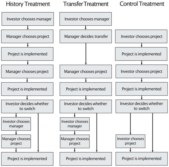
Figure 1.
Design of Treatments.
2.1. Treatments
2.1.1. History
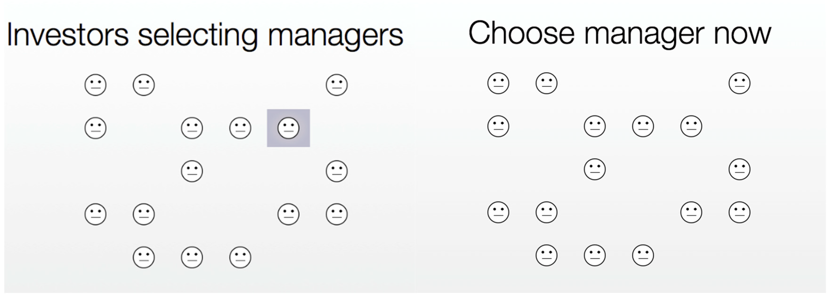
History has twice as many managers as investors, where the role of a participant in the computerized experiment is randomly allocated. At the beginning of each round, an investor chooses a manager from a pool of anonymous managers, who are presented in the form of identical icons spread across the computer screen of the participant (see Figure 2). The position of the icons is randomized in each round, so that the identities of the managers cannot be tracked across rounds. The order in which investors make this choice is randomized anew for each round. Investors who have not yet made a choice and managers who have not yet been chosen see the screen with all eligible icons until they have made a choice or have been chosen, respectively. Icons representing managers who have already been chosen by an investor disappear from the screen one after another. Managers are also informed which icon represents them. Managers who are not chosen by any investor are redirected to a waiting screen7.
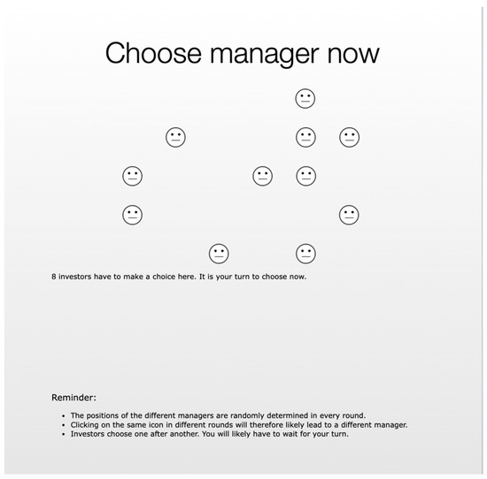
Figure 2.
Choice of Manager.
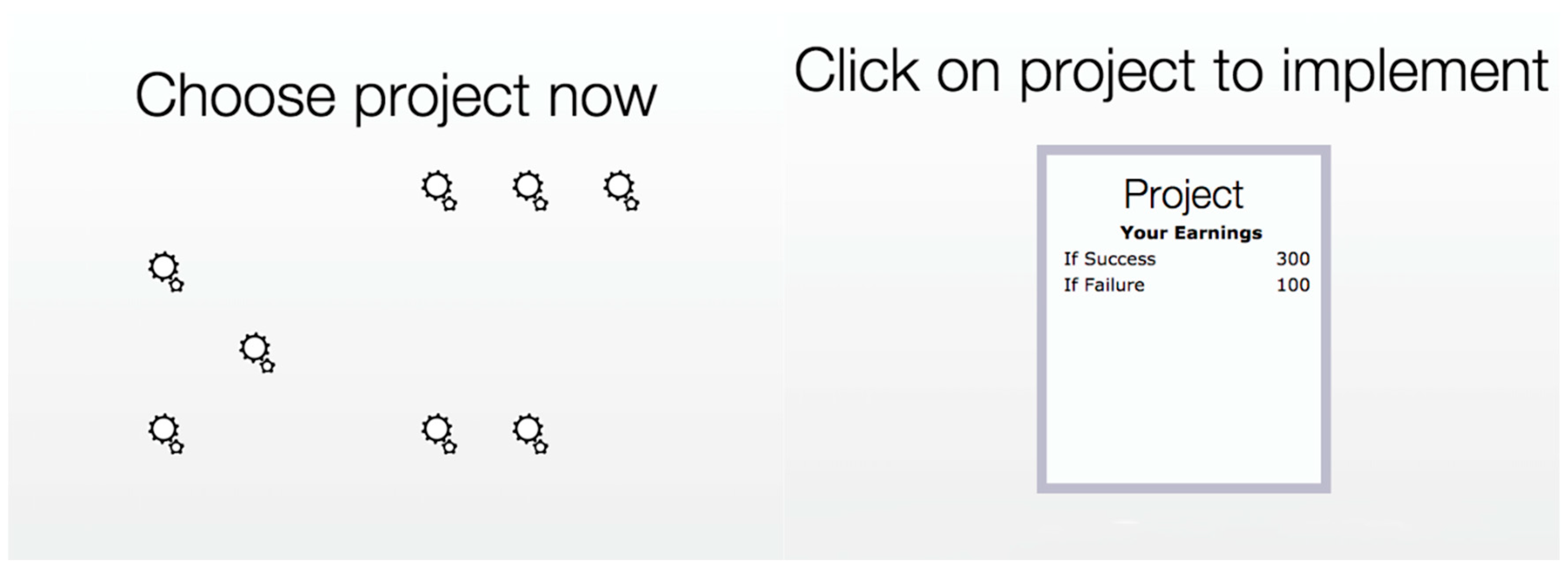
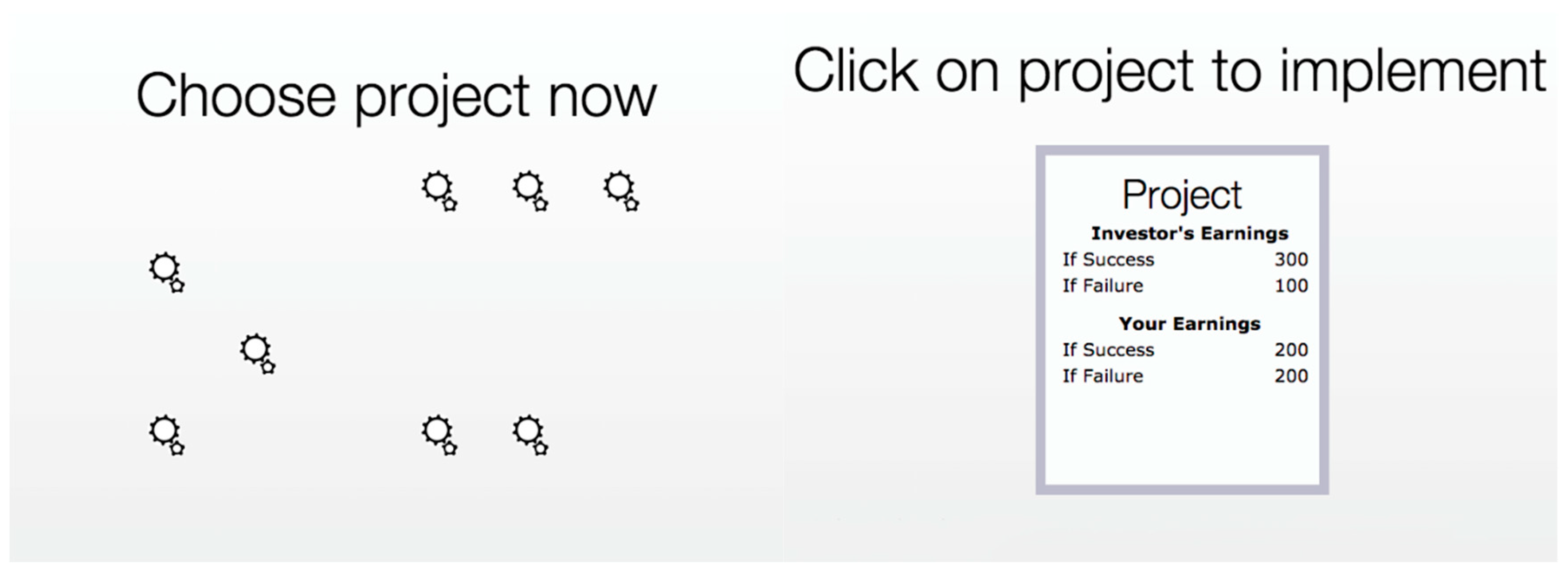
Managers selected by an investor choose one out of eight potential projects. Each project has a success probability of either 1/4 or 3/4. Both types of projects are equally likely, and neither investors nor managers can identify the projects at the time of choosing (their positions on the screen are randomized anew for every decision). The decisions are made in the same order as the choices of the investors, so that a manager who is chosen third is also the third to choose a project. Since all managers select from the same set of projects, for a manager who has been picked last, only one project remains. The project choice screen works in the same way as the investor screen: randomly positioned projects disappear one after another once they are chosen and are no longer available to other managers (see Figure 3). After selecting a project, a manager is asked to “implement” it by clicking on a box that symbolizes the project. Both investor and manager watch a 5-second-long animation resembling the “processing” animation typically found on computers, after which the success or failure of the project is announced.

Figure 3.
Choice of Project.
Following the observation of the project’s outcome by the investor and manager, the manager chooses a second project, which has no relation to the first project in any way. This implies that the success or failure of the first project provides no information at all about the success probability of any later project. The understanding of the last point was tested before the beginning of the experiment.
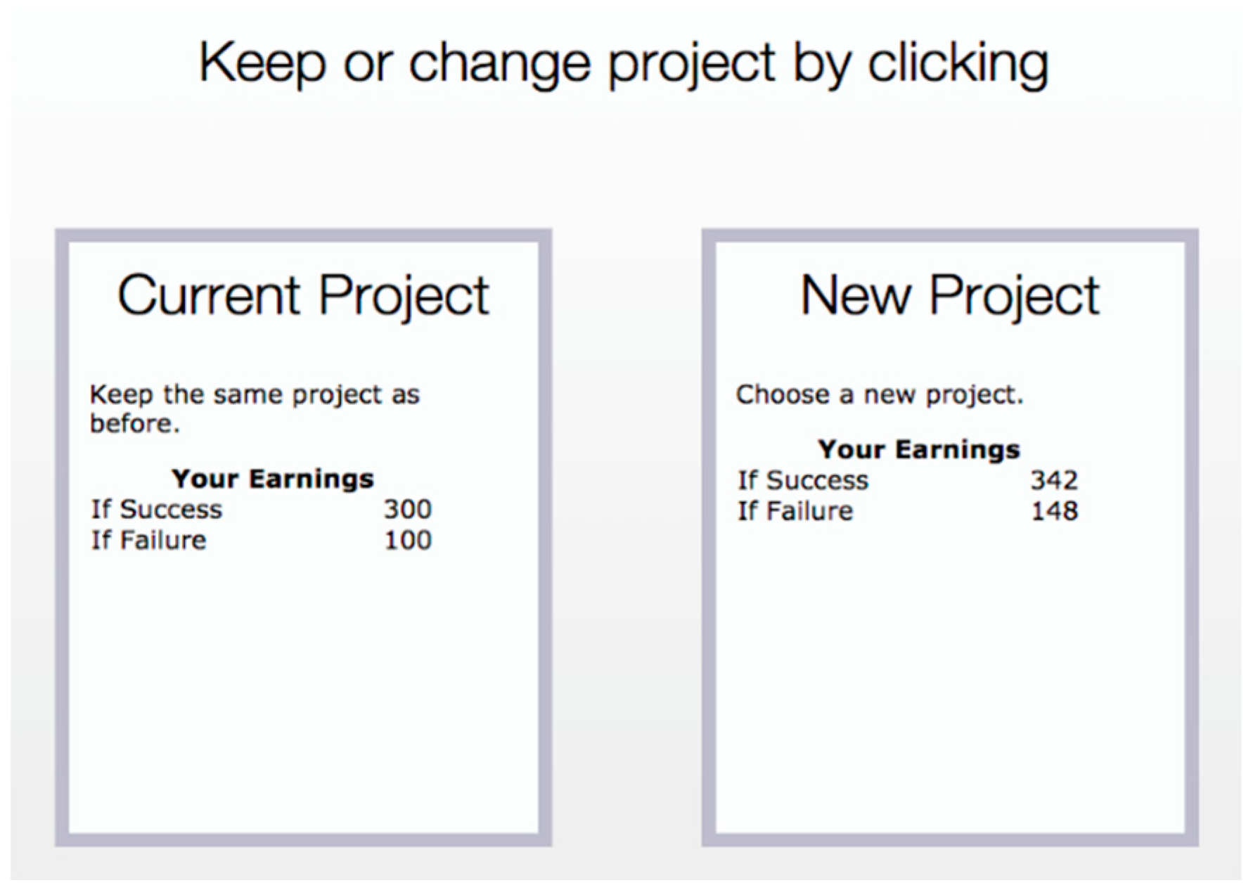
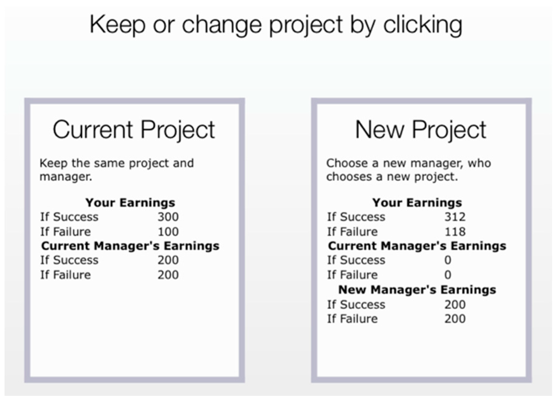
After observing the outcome of this second project, investors are now given the choice to either stay with this project and project manager (re-appointment) or to choose an alternative project manager and project (replacement) using the same method as before. If the investor chooses the first option, the manager is redirected to the implementation screen once more. After the new implementation of the second project, both parties are again informed about its success or failure. Upon choosing to replace the manager, an investor first must wait until all investors have made their decision. Once that is the case, all investors who opted to replace their managers are assigned a new random order and choose a new manager from the pool of managers left unchosen at the beginning of the round. A newly chosen manager then chooses and implements a new project with the same blind procedure as before. After observation of the implementation results, the round ends. There is a total of eight rounds, which only differ in the payoffs of the alternative projects. Payoffs are chosen so as to present the subjects with specific differences in expected value and variances, as explained later in Section 2.2. Every investor faces each combination of returns exactly once across the eight rounds, with the order of the different combinations being randomized to ensure that the distribution of experienced orders was as flat as possible.
2.1.2. Transfer
Transfer follows the same general structure as History, with one important difference. Whereas every round of History starts with a project that is completely unrelated to future projects, this part is now replaced. Instead, managers chosen by an investor are now given the option to transfer money to the investor or not. To that purpose, they are endowed with an extra 10 experimental currency units (ECU) for this transfer. If a manager decides to make that transfer, these 10 units are doubled and the investor’s earnings grow by 20 units.8
After deciding whether to transfer money or not, the manager chooses a project from a pool of eight different projects under the same procedure as in History and implements it in exactly the same way. Thereafter, investors face the same decision as in History, that is, either to stay with the same manager and project or to select a new manager, who then chooses a new project. See Figure 1.
2.1.3. Control
Control eliminates the social element that is present in the two other treatments. Investors now choose and implement their own projects instead of appointing a manager who then chooses and implements a project. Managers are not part of this treatment. Apart from that, this treatment is identical to History. Thus, projects are chosen and implemented in the same way as in the other treatments. See Figure 1.
2.2. Projects
The following explains the earnings of investors and managers and the investor’s (rational and selfish) best response.
A manager who actively manages a project earns 200 ECU, irrespective of the project’s success or failure. Managers who are inactive during the first project in Transfer or the first and second projects in History also receive the same 200 ECU.9 During the final project, inactive managers receive nothing.
Ignoring all social aspects of this experiment for the moment, a payoff-maximizing investor must use relevant past observations as a signal for the underlying success probability of the project to determine the best response.
In every round, an investor can only choose one project. All projects either have a high () or a low () success probability. The ex-ante probability of both types of projects is 50%. Apart from the alternative project that an investor can switch to at the end of a round, all projects generate earnings of 300 ECU in case of a success and 100 ECU in case of a failure. To determine the expected value of a project, we therefore have to calculate the expected value of both types of projects and then combine them to get to the overall expected value:
where we use πH and πL for the payoff of projects with a high or low success probability, denoted by H and L. If the project in question is a completely new project (with payoff π) this implies an expected value of:
The probability of observing the good outcome with payoff 300 is therefore . Once, however, a project has been implemented, its success or failure provides information about this project’s underlying success probability. Using Bayesian updating, we can calculate the probability of the project being of the good type after having observed a successful draw:
Using the same procedure we get , and . Combining Equations (1a,b) and (3), the expected value of a project that was observed to succeed equals:
Similarly, after observing a project to fail its expected value becomes:
Facing the decision whether to implement an old project again or choose a new one, a risk neutral selfish investor would therefore stay with a project that has been successful before (to earn in expectation: E(π|success) = 225) and choose a new manager with an unknown project if the first project implementation was a failure (to earn in expectation: E(π) = 200).
Investors face a more complex situation in the experiment, though. During the first project (in Transfer) or the first and second projects (in History and Control), they earn 300 units in case of success and 100 units in case of failure. The alternative project, however, has other returns, of which investors are informed when they must decide whether to stay with the original (current) manager and project or switch to a new manager and choose a new project. For this reason, the expected value of an original project and an alternative project is, more generally, expressed as follows:
where and , respectively, stand for payoff of the original project with, respectively, high and low success probability, and and for the payoff of the alternative project with, respectively, high and low success probability, while h denotes a particular (success or failure) history of experiences.
Importantly, compared with the original project, the alternative project’s returns are chosen such that they are either equal in their variances, their expected earnings, or both (see Table A1 and Table A2 of Appendix A). The alternative project has higher expected earnings in three cases, and lower expected earnings in one case, while it has a lower variance in two cases, and a higher variance in one case. There are no differences in the remaining cases. Consequently, an (even slightly risk-averse) selfish investor with a perfect ability to perform Bayesian updating will switch in 62.5% to 75% of all cases. Because in five of the eight cases the alternative project either has a higher expected value or a lower standard deviation, the alternative projects are taken as benchmark, both in the Appendix A and the results section below, when describing differences in expected value or standard deviation. For design efficiency, we condition the alternative project returns offered to investors on the success or failure of the original project. Every investor faces each combination of differences in expected value and standard deviation exactly once in different orders.
Calculating the optimal decision in the way outlined above is a challenging task, and we do not expect participants to be very good at that10. In fact, there are reasons to think of it as even beneficial from a design perspective. One is the greater degree of realism that participants face if they are not able to perfectly determine the value of the different options they are facing. Another reason is that situations which present a participant with a higher cognitive load seem more likely to trigger impulsive (emotional) behavior (Duffy & Smith, 2014), particularly in situations relevant for other-regarding behavior (Cornelissen et al., 2011; Schulz et al., 2014). Because the brain processes involved in impulsivity are regarded as relatively effortless (Camerer et al., 2005), this may be seen as an aspect of cognitive efficiency, that is, making decisions with the least amount of mental effort (Hoffman & Schraw, 2010).
2.3. Presentation and Organization
An important aim of the experimental design is to provide an engaging environment for participants, as the blind matching and project choice procedures are fairly impersonal. This motivated us to implement a computerized equivalent of a choice procedure where subjects blindly choose cards indicating their assigned managers and projects in turn. The act of choosing a partner should trigger a stronger engagement than if a partner is purely randomly assigned. A similar logic applies to the project choice of a manager. Participants witness constantly depleting pools of available managers and projects. Furthermore, inspired by computer games, animations are used to illustrate the implementation of projects. For the same reason, finally, the mechanics of choosing whether to stay with a project (and manager) or to choose anew employs a deliberately slow animation to reinforce the notion that this decision, which is our main outcome variable, is of relevance.
Participants’ understanding of the instructions is checked with a quiz covering the most important features of the experiment. After the experiment, a short questionnaire addresses some demographic variables and feelings during the experiment (see Appendix B.2).
Data are from 12 sessions run at the CREED laboratory of the University of Amsterdam in March and April 2015. A total of 222 participants participated. Both Transfer and History comprised 87 participants, a third (29) of whom were concerned investors, while Control had 48 participants, all of them investors. In each session, a random round was selected for payout. Both History and Control paid no show-up fee. The substitution of the first project by a relatively low-value transfer in Transfer motivated a show-up fee of 7 euros in Transfer to ensure satisfactory minimum earnings for participants. The sessions took about 70 min. ECUs were exchanged to euros at a rate of 1 euro per 35 ECU, while average earnings amounted to 16.55 euros.
2.4. Hypotheses
For reasons outlined in the Introduction, an investor’s motivation to stay with a project manager is expected to be relatively stronger (a) if in History the first project was a success instead of a failure, and (b) if in Transfer the manager sent a transfer instead of withholding the money. From now on, a successful first project (in History or, for that matter, Control) or a transfer will be labeled a “positive experience”, and a failure or no transfer a “negative experience”.
In the bonding model discussed in the Introduction, the additional utility of a bond with a manager is represented by the affective tie-value weighted payoff of that manager. Similarly, the hedonic value of the blame or praise felt towards a manager (as in Gurdal et al., 2013) may be seen as an additional utility. Incorporating this additional emotion-related utility, denoted by , into the investor’s utility function, we can compare the expected utility of switching to an alternative manager and project (E(πA), see (6b)) with the expected utility of staying with the original (E(πO), see (6a)) extended with . Using a simple linear function, the extended utility E(U) from each of these two possible options can be written as:
Assuming that is greater after a positive experience than a negative experience, there are more combinations of project payoffs for which is larger than after a positive experience, while the reverse holds for a negative experience. Therefore, we expect a higher (smaller) proportion of investors to stay with their original project and manager in case of a positive (negative) experience.
Because of our focus on the impact of gifts versus other shared experiences, attention will be concentrated on the first project of History. Note, furthermore, that History’s second project, which finds its equivalent in the first project of Transfer and can be expected to have similar effects as ascribed to its first project, is much more difficult to analyze due to being confounded with the calculation of the expected value of proceeding with the original project. Moreover, it does not lend itself well to an inter-treatment comparison since it is not clear how the (emotional) effect from a potential transfer interacts with an additional experience effect of a different type.
Regarding the potential relevance of social preferences models other than the bonding or affective ties model discussed in the Introduction, note that none of the prominent models of altruism, intention-based reciprocity, or those concerning distributional consequences (like inequality aversion or envy models) apply to the situation here (see Appendix C). This is particularly due to the randomness of choices and the equality of managerial earnings in the experimental design. The only exception could relate to giving or withholding a transfer in Transfer.11 But, as argued and further detailed in Appendix C, our results (joint with the findings of Malmendier & Schmidt, 2017) cast doubt on their relevance. See also the Concluding Discussion.
The assumed choice mechanism for the investor, involving Equations (7a) and (7b), is the same in History and in Transfer, the only difference regards the potential motivation. Whereas in History the investor is expected to be more (less) concerned about the earnings of the original manager if they experienced success (failure) in the first project, in Transfer the trigger is whether the manager chose to send the transfer or not, analogous to Malmendier and Schmidt (2017). This leads to our first hypothesis.
Hypothesis 1.
The probability of switching to the alternative project (and a new manager) is lower in the case of a positive experience than after a negative experience.
Merely showing this result is interesting. However, several issues may challenge its theoretical implications. Subjects could be confused by the fact that one project—the first project in Control and in History—is not predictive of the success probability of future projects, while the other project, in fact, is predictive. In addition, a positive experience could generally affect the subjects’ emotional state regarding any familiar project, making them feel more positive about the original project, as opposed to the person who chose it. Moreover, behavior related to a more general type of misunderstanding probabilities, such as the gambler’s fallacy, adds further potential problems. Without a method to control for these effects, we would not be able to attribute the supposed result in Hypothesis 1 to the assumed effect of sharing social experiences. Therefore, in addition to the first hypothesis, we also require that the effect size of the different experiences is larger in History and Transfer than in Control. Additionally, in History, as argued in the Introduction, transfers are more directly emotionally affecting an investor than a project outcome. This leads to our second hypothesis.
Hypothesis 2.
The effect of different experiences on the probability of switching follows the order Control < History < Transfer.
3. Results
Table 1 presents demographic data about the participants in the experiment and specifies the histories that the investors in the different treatments experienced prior to making their decision about staying with the same project (and manager) or not. Note that a “positive experience” (denoted by “+”) now also comprises the experience of a successful first project in Control, and a “negative experience” (denoted by “−”) a failure in that case. For notational simplicity, a success or failure of the project prior to the switch or stay decision is also indicated with, respectively, a “+” and a “−”. An “experienced history” contains both results. Thus, for example, a negative experienced history is indicated by “−/−”. The distribution of positive experiences (the sum of +/+ and +/− histories) and negative experiences (the sum of −/+ and −/− histories) in Control is perfectly balanced at 192 each by design, while in History the balance is not perfect because some sessions were run with only 18 or 21 instead of 24 participants due to low show-up, leading to a success rate of 48.7%. Experienced histories in Transfer are a function of the participants’ decision making: managers sent the voluntary transfer in 166 out of 232 possible cases, a grand total of 71.6%. This is close enough to our optimal distribution of 50% to allow us to make statements about the reaction of investors to either receiving the transfer or not.12

Table 1.
Demographic Data and Experienced Histories.
Pooling treatments, there is no significant change in the investors’ switching rate across the 8 rounds of the experiment (Figure 4).13 In Transfer, there appears to be a slight, but only weakly significant, increase in the second half of the experiment.14
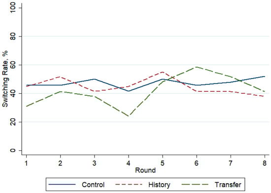
Figure 4.
Switching Rate across Rounds by Treatment.
We begin our investigation into the investor behavior with a simple question: Does the experience at the very beginning of a round matter? Figure 5a shows the proportions of investors choosing a new project (and manager) after a negative experience and after a positive experience in the different treatments. Recall that a perfectly selfish and Bayesian investor will switch in 62.5% to 75% of all cases, irrespective of the experience or treatment. A switching rate of 53.6% shows up in case of a negative experience, and 38.4% in case of a positive experience; a highly significant difference (p < 0.001).15 This result confirms Hypothesis 1:
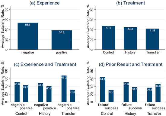
Figure 5.
Switching Rates by Experience, Treatment, and Prior Result.
Result 1.
A positive experience leads to a significant drop in switching rates relative to a negative experience, confirming Hypothesis 1.
Next, Figure 5b shows the overall switching rates in the different treatments, revealing a constant decrease going from Control to History and Transfer. These differences are not significant, however.16
A natural next step is to compare switching rates relative to types of experience in the separate treatments; see Figure 5c. While the difference in switching rates is substantial in Transfer (36.9 percentage points), the difference in History (8) is not only nigh-identical to Control (8.3), but even slightly smaller. The only treatment in which the investors’ behavior differs significantly between experiences is Transfer.
Another dimension for comparing investors’ decisions is the outcome of the project implemented just prior to the switch or stay decision, labeled the “prior project” from now on. Recall that the original prior project can be reimplemented by sticking with the original manager. The expected value of the alternative project is adjusted to the expected value of a new implementation of the original project, as can be calculated using Bayesian updating. Nevertheless, a positive experience effect of the original project might still be expected. This is not observed, however, as the difference decreases between Control and History, and even reverses in Transfer (Figure 5d; the only significant difference between prior results is found in Control).
The ability of participants to correctly perform Bayesian updating is not at the core of our analysis and is not necessary for the interpretation of our experimental findings. Nevertheless, note that investors have a monetary incentive to switch projects more often if it is relatively beneficial to do so. Figure 6 distinguishes the different alternatives that investors faced in the experiment. Pooling all treatments, there seems to be a discernible effect when comparing the most extreme cases of positive or negative differences in expected value (19.8%, p < 0.01).17 However, there is no monotonic increase in switching rates with increasing differences in expected value. The same is true for the projects with different variances, where one would expect an increasing switching rate, the lower the variance of the alternative project.
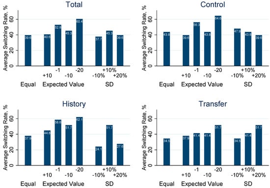
Figure 6.
Project Switching by Dilemma Type. Original and alternative projects either have the same expected value and variance or differ in one of these two dimensions. Labels refer to the situation in which the respective values for the original project differ from the alternative project (taken as the benchmark); the other dimension is always identical between projects. For example, in the case of the expected value −20, the original project has an expected value that is 20 units lower than the alternative project, implying that switching is the best response for a purely self-interested investor. Expected value differences are in absolute values, while differences in standard deviation are in relative values, rounded to full percentage points.
So far, we have only compared the investors’ behavior relative to their different experiences within the three treatments. Hypothesis 2 goes one step further. There, we hypothesized that the effect of different experiences on the switching rate should be smallest in Control and largest in Transfer, with History in the middle. Figure 5c indeed suggests that the difference is largest in Transfer. Comparing Control and History, however, the difference is smallest in Control. To come to a more conclusive statement, we use panel (logit) regressions in which treatments are interacted with experiences (Table 2). The switching probability in Control after a negative experience and prior result forms the baseline. Irrespective of the specification, the results fall in line with the first impression from Figure 5c. The coefficient of the interaction term between Transfer and a positive experience is always negative and significant at the 1%-level, while the coefficient of the interaction between History and a positive experience is not significant.
Table 2.
Investor Decision Regressions (logit model).
This impression is confirmed by running chi-square tests over the differences in switching rates predicted by the (logit) coefficients in the different treatments.18 Moreover, a regression similar to specification (4) using History, instead of Control, as baseline (5) confirms the absence of a difference in the differences between Control and History, while there is a significant negative interaction of Transfer with a positive experience. In conclusion, only partial evidence for Hypothesis 2 obtains:
Result 2.
Switching rates after different experiences are not significantly different between Control and History, failing to support a relevant part of Hypothesis 2. However, as hypothesized, in the Transfer treatment, the difference in switching rates is significantly larger than in the Control and History treatments.
Additional significant findings relate to the results of the prior project and differences in the expected values of the original and alternative projects. A positive outcome of the prior project leads to a lower switching rate, while a difference between the expected values of the original project and the alternative project affects switching in the expected direction also (that is, the higher the expected value of the original project, the less switching is predicted).19
Our next issue concerns the decision-making time of investors. Interestingly, the decision times in the two social treatments, History and Transfer, are significantly—and more than 40%—longer than in Control (Figure 7).20 The difference in decision times between History and Transfer, on the other hand, is negligible at 0.5 s. This result appears to be driven by a smaller proportion of investors making their decision very quickly (see density estimate in Appendix A Figure A2) and is stable across rounds (see Appendix A Figure A3). A panel regression confirms these findings (Appendix A Table A4). Interestingly, decision speeds do not seem to be correlated with either the decision made by the investor or the absolute difference in the expected value or variance between the two projects.21
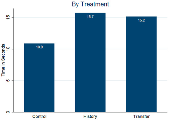
Figure 7.
Investor Decision Times by Treatment (seconds).
Finally, as part of the post-experiment questionnaire, managers were asked for the most important reason why they sent a transfer, if they sent any. In line with the findings of Malmendier and Schmidt (2017), a strategic selfish motivation dominates, with 86% (50 out of 58, Question 6 in Appendix B.2.1) hoping that it would make the investor stay with their project; only 7 wanted to be kind, and only 1 mentioned the group income (efficiency) as motive. Note that the absence of kindness is no problem for the affective ties model (ATM), because it focuses on directed actions and the emotions they trigger, irrespective of the underlying motivation (intentions).
Regarding the emotionality of investors, the questionnaire comprised a set of questions concerning their affective response to either receiving a transfer from a manager (in Transfer) or experiencing a successful first project with a manager (in History).22 More specifically, they were asked (with a 5-point intensity scale) whether they felt a positive emotion and a sense of obligation towards such a manager, and whether they were more likely to stay with that manager (and project). Figure 8 shows the distribution of their answers in the two treatments. Regarding the emotion question, the distribution of answers in History is bimodal, with 33% choosing 1, the lowest possible score on the intensity scale. In Transfer 0% chose 1, while 75% chose a value of 4 or 5. This picture is confirmed by the questions regarding the feeling of a sense of obligation towards the manager and the direct question concerning their likelihood to stay with such a manager. There is always a lot more mass on the upper part of the distribution in Transfer compared to History. In all questions, average scores are significantly higher in the former, with p-values below 0.001. This suggests that emotionality indeed played a much stronger role in Transfer than in History, as expected in the Introduction.
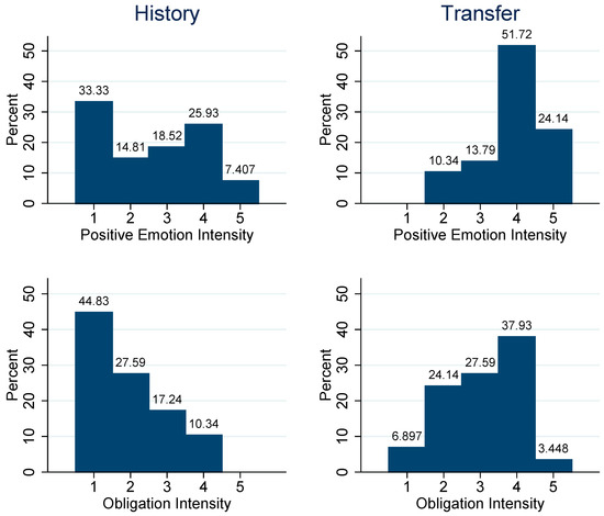
Figure 8.
Questionnaire: investor scores on emotion, obligation, and likelihood to stay with a project manager after a positive experience. Two subjects answered they had not experienced success in the first project when asked for their emotion rating, leaving 27 observations. In all other cases, we have answers from all 29 investors in both treatments.
Correlations between the intensity scores regarding the emotion, obligation feeling and likely to stay questions, for History and Transfer, show that the only significant correlations are between emotion and obligation feeling in History (0.54, p = 0.004) and between emotion and likely to stay in Transfer (0.41, p = 0.027), whereas obligation feeling and likely-to-stay are not significantly correlated in either treatment.23 These findings suggest that the feeling of an obligation plays a relatively stronger role in History, and “likely-to-stay” plays a stronger role in Transfer. Joint with the observed stay-reaction to positive experiences only in Transfer (Table 2), it is not surprising that investor decision regressions including these questionnaire data show that the emotion and likely to stay scores are predictive of the stay-reaction in that case (see Appendix A Table A6).24 Interestingly, in these regressions, obligation shows a significant switch-reaction to negative experiences,25 but only a marginally significant stay-reaction (of similar size) to positive experiences. Although Gurdal et al. (2013) do not measure specific emotions, our observations seem to provide some support for their unjustified blame model, discussed in the Introduction. The fact that this does not show up in the switching rate regressions (Table 2) seems due to the relatively small number of participants reporting relatively high scores (only 8/29 scoring at least 3 on the 5-point intensity scale).
Gurdal et al. (2013) see blame as an emotional expression that “can be rationally supported as part of a normative morality” (op. cit., pp. 1208–1209). A relationship with norms differentiates it from the observed bonding involved in likely-to-stay in Transfer.26 Although one may feel obliged upon receiving a gift from a stranger, the affective tie that it creates—which endogenizes a preference to take an interaction partner’s welfare/utility into account (see Equation (7a))—loosens the feeling of an obligation to reciprocate (see Silk, 2003, and references therein).27 Recall, in this context, the lack of correlation between likely-to-stay and obligation.
4. Concluding Discussion
Our experimental results show a clear differential impact on an investor-manager relationship of a context where the manager has the option to provide a transfer (gift) to the investor who randomly selected the manager (Transfer), compared to a context where the two only share an experience concerning the resolution of a project randomly selected by the manager (History). In Transfer, compared to a non-social yet otherwise comparable context (Control), the rate of switching to a new manager and project after a positive experience (receiving a transfer) is smaller. In stark contrast, in History, no such change is observed.
Like Malmendier and Schmidt (2017), we find a strong (transfer vs. no transfer) gift effect that reaches almost 37 percentage points (44 in their paper).28 This is despite the fact that decision-makers in our case only face the decision to stay or switch after an intermediate project. Not only does this project end with the cognitively strenuous task of having to evaluate the relative value of two project options, but it also adds to the passing of a non-negligible amount of time between transfer and decision. This makes our study a much more demanding test of a gift effect than the one investigated by Malmendier & Schmidt. Our experimental design further differs from that experiment in that, in our case, the decision is one about an ongoing relationship, as opposed to first-time choosing between two unknown producers. The comparison with a non-social, yet otherwise comparable treatment makes for another difference.
Although our findings are consistent with a bonding model as proposed by Malmendier & Schmidt—while none of the prominent social preferences models, like intention-based reciprocity or inequality aversion, are directly applicable (Appendix C)—we question their requirement of a perceived intention and their suggestion that the response is triggered by an (internalized) norm-related obligation to repay (see Introduction). Moreover, and importantly, their model lacks a theoretical bonding mechanism. The affective ties model (ATM) that we propose for explanation provides such a mechanism. It requires a hedonic action for bonding to occur, irrespective of its underlying motivation (van Dijk & van Winden, 1997; van Winden, 2023). The above findings for Transfer and History are, therefore, in line with that model. The self-reported strategic selfish motivation for sending a transfer and the feeling-related responses in the post-experimental questionnaire are supportive in this respect. After a positive experience, participants in Transfer are much more emotional than in History and report being much more likely to stay with the original manager. Interestingly, the feeling of an obligation also occurs in Transfer, but it is not correlated with the self-reported likelihood to stay in reaction to a transfer. This makes sense as it badly fits an affective tie (feeling obliged for a small gift is for strangers, not for friends) in contrast to a social norm. The reason is that if at all an internalized norm is at stake—for, note that a transfer is neither asked for nor can it be rejected—it will have to compete mentally with tie formation. Whereas the latter provides a direct hedonic motivation, the motivation for internalized norm reciprocity runs indirectly via the anticipation of emotions like guilt or shame in case of violating the normative interests of valued norm instillers (van Winden, 2023). Consistently, the feeling of an obligation is clearly correlated with emotional intensity in History only. Furthermore, in History, we also find a clear negative effect of feeling an obligation in the case of a negative experience (project failure), which reminds us of the unjustified blame observed in Gurdal et al. (2013). However, this feeling appears too weak among the participants to have an effect at the group level.
The participants’ understanding of the relative values of the different projects presented to them was at best tenuous (Figure 6). At least in Control, one would expect a dramatic difference in switching rates between the situation in which switching is advantageous compared to when it is disadvantageous. This is not in and of itself a problem for our comparative analysis, however, as the dilemmas that participants faced are identical across treatments. Furthermore, substantial evidence exists suggesting that a complex decision-making task (cognitive load) need not stand in the way of more intuitive and emotional mechanisms like ATM and, on the contrary, actually gives these a better chance (see discussion and references in Section 2.2). Thus, there is little reason to believe that the intensity of an investor’s loyalty towards a manager is weakened by the complexity of the situation.
Illusion of control (Langer, 1975), on the other hand, might play a role in the comparison between the Control treatment and the two social treatments. Investors in the Control treatment choose the lottery directly, rather than through a manager, hypothetically giving them a greater sense of control. It is, however, unclear in which direction this effect would go, since this applies to both the original and alternative projects.
Another potential problem referred to in the Introduction concerns the gambler’s fallacy. This well-known fallacy, however, should not lead to any differences in average switching behavior between treatments, as the experience prior to the switch is distributed the same.
By choosing an experimental protocol that clearly separates the two roles of investor and manager, we carefully avoided any complex behavioral effects that might arise otherwise. Mixing roles would have aided experimental efficiency by creating more observations, but, as has been shown for dictator-games, at potential cost (Grech & Nax, 2020). This only holds if all investors were aware that roles would not be mixed later, which we have no reason to doubt.
A remarkable difference between the social treatments (History and Transfer) and the non-social treatment (Control) concerns the investor’s time involved in making the stay or switch decision, which is substantially longer—while very similar—in the former. Although it is not clear at this stage what exactly the reason is, a plausible driving factor concerns the extended utility of an investor in that situation, due to an additional norm and/or interaction partner’s payoff-related utility component.
Another issue deserving further research regards the question of what counts as a relevant action for bonding.29 What seems essential is that the behavior of a protagonist (manager) has an associated hedonic impact on the decision maker (investor). Through the randomization in our design, a project’s success or failure provides minimal (if any) direct information about the type of manager the investor is dealing with, which is key in the affective tie model.
A further avenue for future research concerns the controlling for participants’ initial prosocial attitudes towards interaction partners, based on past interaction experiences in similar situations, referred to as generalized tie value above (see Note 3). A practical measure of which would be their social value orientation, a frequently used psychological measure in the study of social dilemmas (for some reviews, see: Au & Kwong, 2004; Bogaert et al., 2008; Murphy et al., 2011).
In conclusion, this study provides clear experimental support for the relevance of social preference dynamics (bonding) in an investor-manager relationship, based on (even relatively minor) direct hedonic interaction experiences. Only weak evidence is obtained for unjustified blame or praise.
Author Contributions
Conceptualization, M.O.H. and F.v.W.; Methodology, M.O.H. and F.v.W.; Software, M.O.H.; Formal analysis, M.O.H.; Investigation, M.O.H. and F.v.W.; Resources, F.v.W.; Data curation, M.O.H.; Writing—original draft, M.O.H.; Writing—review & editing, M.O.H. and F.v.W.; Visualization, M.O.H.; Supervision, F.v.W.; Project administration, F.v.W.; Funding acquisition, F.v.W. All authors have read and agreed to the published version of the manuscript.
Funding
This research was funded by the Research Priority Area Behavioral Economics of the University of Amsterdam, grant number 201502121002.
Data Availability Statement
Data from the experiment and code used for the analysis found in the paper is available publicly at https://github.com/mohoyer/investor-manager-relationship (accessed on 14 May 2025).
Acknowledgments
For useful comments on the previous version of this paper (“Investors have feelings too”) we are thankful to participants at ESA, FUR and CCC meetings and at seminars at the Tinbergen Institute and the University of Amsterdam, as well as two reviewers of a journal. Financial support from the Research Priority Area Behavioral Economics of the University of Amsterdam is gratefully acknowledged. For additional analysis we are grateful to William Backes.
Conflicts of Interest
Author M.O.H. was employed by the candidate select GmbH company. The remaining authors declare that the research was conducted in the absence of any commercial or financial relationships that could be construed as a potential conflict of interest.
Appendix A. Additional Figures and Tables
Table A1.
Possible situations after an experienced failure.
Table A1.
Possible situations after an experienced failure.
| Original Project | Alternative Project | Comparison Between Projects | ||||||||||
|---|---|---|---|---|---|---|---|---|---|---|---|---|
| EV Ex Ante | EV After Failure | SD Ex Ante | SD Ex Post | Earnings If Success | Earnings If Failure | Expected Value | Standard Deviation | Difference EV * | Difference SD ** | |||
| Same EV/SD | 200 | 175 | 100 | 96.8 | 272 | 78 | 175 | 97 | 0 | 0% | ||
| Different EV | 200 | 175 | 100 | 96.8 | 262 | 68 | 165 | 97 | 10 | 0% | ||
| Different EV | 200 | 175 | 100 | 96.8 | 273 | 79 | 176 | 97 | −1 | 0% | ||
| Different EV | 200 | 175 | 100 | 96.8 | 282 | 88 | 185 | 97 | −10 | 0% | ||
| Different EV | 200 | 175 | 100 | 96.8 | 292 | 98 | 195 | 97 | −20 | 0% | ||
| Different SD | 200 | 175 | 100 | 96.8 | 283 | 67 | 175 | 108 | 0 | −10% | ||
| Different SD | 200 | 175 | 100 | 96.8 | 263 | 87 | 175 | 88 | 0 | 10% | ||
| Different SD | 200 | 175 | 100 | 96.8 | 256 | 94 | 175 | 81 | 0 | 20% | ||
* The difference in expected value is expressed as the absolute difference in ECU by which the original project differs from the benchmark alternative project. ** The difference in standard deviation is the relative difference in variance of the original project compared to the alternative project, rounded to full percentage points.
Table A2.
Possible situations after an experienced success.
Table A2.
Possible situations after an experienced success.
| Original Project | Alternative Project | Comparison Between Projects | ||||||||||
|---|---|---|---|---|---|---|---|---|---|---|---|---|
| EV Ex Ante | EV After Failure | SD Ex Ante | SD Ex Post | Earnings If Success | Earnings If Failure | Expected Value | Standard Deviation | Difference EV * | Difference SD ** | |||
| Same EV/SD | 200 | 225 | 100 | 96.8 | 322 | 128 | 225 | 97 | 0 | 0% | ||
| Different EV | 200 | 225 | 100 | 96.8 | 312 | 118 | 215 | 97 | 10 | 0% | ||
| Different EV | 200 | 225 | 100 | 96.8 | 323 | 129 | 226 | 97 | −1 | 0% | ||
| Different EV | 200 | 225 | 100 | 96.8 | 332 | 138 | 235 | 97 | −10 | 0% | ||
| Different EV | 200 | 225 | 100 | 96.8 | 342 | 148 | 245 | 97 | −20 | 0% | ||
| Different SD | 200 | 225 | 100 | 96.8 | 333 | 117 | 225 | 108 | 0 | −0.1 | ||
| Different SD | 200 | 225 | 100 | 96.8 | 313 | 137 | 225 | 88 | 0 | 10% | ||
| Different SD | 200 | 225 | 100 | 96.8 | 306 | 144 | 225 | 81 | 0 | 20% | ||
* The difference in expected value is expressed as the absolute difference in ECU by which the original project differs from the benchmark alternative project. ** The difference in standard deviation is the rel. difference in variance of the original project compared to the alternative project, rounded to full percentage points.
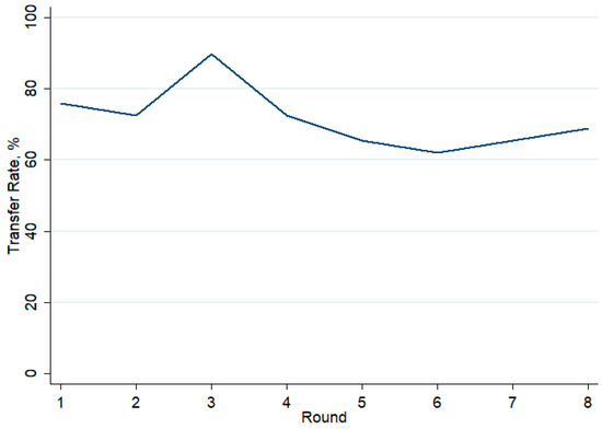
Figure A1.
Transfer Decisions over Different Rounds.
Table A3.
Investor Decision Regressions (probit model).
Table A3.
Investor Decision Regressions (probit model).
| Investor Switches Project | |||||
|---|---|---|---|---|---|
| (1) | (2) | (3) | (4) | (5) | |
| Control | 0.158 (0.97) | ||||
| History | −0.074 (−0.48) | −0.113 (−0.71) | −0.158 (−0.97) | ||
| Transfer | 0.430 * (2.24) | 0.368 (1.90) | 0.363 (1.85) | 0.521 * (2.43) | |
| Positive Experience | −0.216 (−1.66) | −0.435 *** (−4.77) | −0.307 * (−2.68) | −0.310 * (−2.31) | −0.211 (−1.22) |
| Control × Positive Experience | −0.100 (−0.46) | ||||
| History × Positive Experience | 0.009 (0.05) | 0.085 (0.39) | 0.100 (0.46) | ||
| Transfer × Positive Experience | −0.749 ** (−3.21) | −0.631 ** (−2.68) | −0.612 ** (−2.59) | −0.711 ** (−2.73) | |
| Prior Result Positive | −0.435 *** (−4.83) | −0.424 *** (−4.69) | −0.439 *** (−4.81) | −0.439 *** (−4.81) | |
| Expected Value Difference | −0.017 ** (−3.18) | −0.016 ** (−3.00) | −0.016 ** (−2.86) | −0.0156 ** (−2.86) | |
| SD Difference | 0.003 (0.48) | 0.002 (0.38) | 0.002 (0.34) | 0.002 (0.34) | |
| Round | 0.011 (0.58) | 0.011 (0.58) | |||
| Female | 0.041 (0.40) | 0.041 (0.40) | |||
| Age | 0.006 (0.32) | 0.006 (0.32) | |||
| Economics Student | −0.123 (−1.12) | −0.123 (−1.12) | |||
| Choice number | −0.033 (−1.60) | −0.033 (−1.60) | |||
| Constant | 0.041 (0.43) | 0.278 ** (3.22) | 0.248 * (2.22) | 0.287 (0.63) | 0.129 (0.29) |
| Individuals | 106 | 106 | 106 | 106 | 106 |
| N | 848 | 848 | 848 | 848 | 848 |
Random effects model with z-statistics in parentheses, using robust standard errors. *: p < 0.05, **: p < 0.01, ***: p < 0.001.
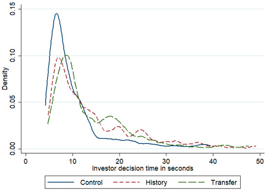
Figure A2.
Decision Time Density Estimate (ignoring outliers above 50 s; Epanechnikov kernel with bandwidth of 1 s).
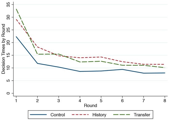
Figure A3.
Decision Time in Different Rounds.
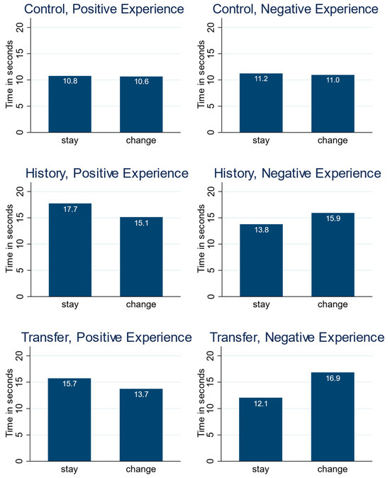
Figure A4.
Decision Time by Experience.
Table A4.
Investor Decision Time Regression.
Table A4.
Investor Decision Time Regression.
| Decision Time | ||||
|---|---|---|---|---|
| (1) | (2) | (3) | (4) | |
| History | 3.595 * (2.54) | 3.440 * (2.43) | 3.686 ** (2.62) | |
| Transfer | 4.267 * (2.55) | 4.180 * (2.49) | 4.734 ** (2.94) | |
| Positive Experience | −0.389 (−0.35) | 0.485 (0.63) | −0.622 (−0.56) | −0.606 (−0.60) |
| History × Positive Experience | 2.523 (1.39) | 2.801 (1.55) | 2.619 (1.58) | |
| Transfer × Positive Experience | 0.110 (0.06) | 0.292 (0.15) | −0.831 (−0.47) | |
| Investor Switches Project | −0.360 (−0.46) | −0.376 (−0.48) | −0.106 (−0.15) | |
| Prior Result Positive | −1.490 * (−1.97) | −1.587 * (−2.10) | −1.599 * (−2.32) | |
| Absolute Expected Value Difference | 0.00198 (0.03) | 0.000921 (0.02) | −0.00277 (−0.05) | |
| Absolute SD Difference | −0.0586 (−0.95) | −0.0586 (−0.95) | −0.0614 (−1.10) | |
| Round | −1.843 ** (−12.80) | |||
| Female | −0.0618 (−0.07) | |||
| Age | −0.208 (−1.29) | |||
| Economics Student | 1.558 (1.53) | |||
| Choice Number | −0.0132 (−0.08) | |||
| Constant | 11.10 *** (12.72) | 14.32 *** (13.66) | 12.48 *** (10.42) | 24.48 *** (5.81) |
| Individuals | 106 | 106 | 106 | 106 |
| N | 848 | 848 | 848 | 848 |
Random effects model with z-statistics in parentheses, using robust standard errors. *: p < 0.05, **: p < 0.01, ***: p < 0.001.
Table A5.
Correlations between Questionnaire Answers.
Table A5.
Correlations between Questionnaire Answers.
| History | Transfer | |
|---|---|---|
| Emotion and Obligation | 0.54 (0.0038) ** | 0.35 (0.0598) |
| Obligation and Likelihood to Stay | 0.15 (0.4260) | 0.06 (0.7430) |
| Emotion and Likelihood to Stay | 0.11 (0.5742) | 0.41 (0.0266) * |
*: p < 0.05, **: p < 0.01.
Table A6.
Investor decision regressions.
Table A6.
Investor decision regressions.
| Investor Switches Project | |||
|---|---|---|---|
| (1) | (2) | (3) | |
| Transfer | −0.0152 (−0.05) | −0.203 (−0.73) | 0.396 (1.47) |
| Positive Experience | 0.134 (0.25) | −0.0514 (−0.10) | 0.167 (0.35) |
| Result previous project | −0.00932 (−0.05) | −0.0217 (−0.11) | −0.0346 (−0.17) |
| Expected Value Difference | −0.0296 * (−2.39) | −0.0288 * (−2.36) | −0.0276 * (−2.26) |
| SD difference | 0.0112 (0.91) | 0.0137 (1.13) | 0.0135 (1.12) |
| Emotion | 0.210 (1.55) | ||
| Positive Experience × Emotion | −0.333 * (−2.11) | ||
| Obligation | 0.424 ** (2.71) | ||
| Positive Experience × Obligation | −0.337 (−1.88) | ||
| Likelihood to Stay | 0.0304 (0.22) | ||
| Positive Experience × Likelihood to Stay | −0.409 * (−2.53) | ||
| Constant | −0.438 (−0.97) | −0.800 * (−1.99) | −0.0670 (−0.17) |
| Individuals | 56 | 58 | 58 |
| N | 448 | 464 | 464 |
Random effects model with z-statistics in parentheses, using robust standard errors. *: p < 0.05, **: p < 0.01.
Appendix B. Instructions and Questionnaires
Appendix B.1. Instructions
Appendix B.1.1. Control Treatment
- Welcome to This Experiment
In this experiment you can earn a substantial amount of money. Your earnings will be paid to you privately and confidentially right after the end of the experiment. We will be using an Experimental Currency Unit (ECU), which will be exchanged to euros at a rate of 1 euro per 35 ECU.
Your decisions in this experiment will be recorded anonymously and neither participants nor experimenters will be able to link your decisions to you after the experiment.
You must not communicate with any of the other participants during the experiment. If you have a question raise your hand and wait until we come to your desk.
- Instructions
In this experiment you are an investor.
An investor chooses one from eight possible projects. Investors make their choices one after another in random order and there are up to eight investors in one group. Each project can either succeed or fail.
The investor does not know the exact probability with which a project will succeed or fail when choosing it. However, there are only two types of projects:
- Type 1 succeeds with a probability of 75% (meaning it succeeds on average in three out of four cases);
- Type 2 succeeds with a probability of 25% (on average in one out of four cases).
Each type of project is equally likely to occur.
A successful project generates more earnings for an investor than a failed project, the details of which will be explained later. You are always informed about your potential earnings before the project is implemented, but you never know for certain whether it is of the type with a high or a low success probability.
In practice the experiment will be presented to you as follows. Investors choose a project from a screen with eight different projects, as illustrated by the left screenshot below. They do so in random order. Half of the projects are of the type that is more likely to be successful and the other half is of the type that is less likely to be successful, but no investor knows which project is of which type. Once all investors have chosen a project, you implement your project by clicking on the box in the right screenshot. You are then told whether your own project was a success or a failure.
After the first project has been implemented, investors select a new project, which again is equally likely to be of the type that has a high (75%) or low (25%) success probability. The implementation of the project will follow the same procedure as before.
- The third project
Finally, a third project is to be implemented. However, in this case the situation changes: You can either proceed with the second project or choose to change to a new project.
If you choose to proceed with the second project, it is going to be implemented once more. It will still have the same success probability as before, meaning that if you chose a project with a high success probability of 75% it still has that success probability of 75%, and similarly for a project with a low success probability of 25%.
Of course, a previously successful project need not necessarily have to be of the high success probability type, and an unsuccessful project need not necessarily have to be of the low success probability type.
If, instead, you choose to change to a new project, you will choose from a set of 8 new projects. These projects are again equally likely to be of the high (75%) or low (25%) success probability type.
Note that new projects can have different earnings, both if successful or unsuccessful. You will be informed about the new earnings before choosing whether to stay with the current project or switching to a new one.
- Earnings from projects
For each of the first two projects investors earn 300 ECU in case of success and 100 in case of failure.
The third project can have different earnings. Here is an example of the screen that the investor may see when making her or his decision at that stage:
- Note
Note that a project that has been successful in the past is more likely to be of the type that is successful with 75% probability than with 25% probability. In the same way, a project that was unsuccessful in the past is more likely to be of the type that succeeds with 25% probability. In contrast, if you change to a new project, you will have no information about its success probability other than that each type is equally among the 8 new projects.
Furthermore, if you have reason to believe that a project is successful with 75% probability it is possible that it is a relatively valuable project, even if the amount of money that you earn in case of a success and in case of a failure are both lower than in another project.
- Rounds and payment
Each round of the experiment consists of the three projects described before. In total, there will be 8 rounds, each with different combinations of earnings for the different projects in case of success and failure.
The positions of the different projects on the screen on which they are chosen are randomly determined in each round, so you cannot track them throughout the different rounds.
After the end of the experiment we will randomly draw one of the 8 rounds. Your earnings in that round will determine your payment. Your payment from other rounds will be zero.
- Summary
- The experiment consists of eight different rounds.
- In each round you will have to choose two projects that may either succeed or fail with a certain probability.
- For the third and final project in a round you can decide either to stay with your current project or change to a new project.
- For each of the first two projects you will earn 300 ECU in case of success and 100 ECU in case of failure. The third project can have different earnings.
- Only one of the eight rounds (with three projects each) will be randomly selected for payment.
Appendix B.1.2. History Treatment
- Welcome to this experiment
In this experiment you can earn a substantial amount of money. Your earnings will be paid to you privately and confidentially right after the end of the experiment. We will be using an Experimental Currency Unit (ECU), which will be exchanged to euros at a rate of 1 euro per 35 ECU.
Your decisions in this experiment will be recorded anonymously and neither participants nor experimenters will be able to link your decisions to you after the experiment.
You must not communicate with any of the other participants during the experiment. If you have a question raise your hand and wait until we come to your desk.
- Instructions
In this experiment you are either an investor or a project manager. You will be informed about your role at the beginning of the experiment and your role will stay the same throughout the whole experiment.
There are twice as many project managers as investors in this experiment. Each investor chooses between different project managers. Investors make their choices one after another in random order and there are up to eight investors.
After each investor has chosen a manager, the project manager chooses one from eight possible projects. Each project can either succeed or fail. A successful project earns more money for the investor than an unsuccessful one.
After this decision the project manager chooses one from eight possible projects. Each project can either succeed or fail. A successful project earns more money for the investor than an unsuccessful one.
Neither the investor nor the project manager knows the exact probability with which a project will succeed or fail when choosing it. However, there are only two types of projects:
- Type 1 succeeds with a probability of 75% (meaning it succeeds on average in three out of four cases);
- Type 2 succeeds with probability 25% (on average in one out of four cases).
Each type of project is equally likely to occur.
A successful project generates more earnings for an investor than a failed project, the details of which will be explained later. You are always informed about your potential earnings before the project is implemented, but you never know for certain whether it is of the type with a high or a low success probability.
In practice the experiment will be presented to you as follows. You first see a screen with all the available project managers. One after another—in random order—the investors get to choose between different managers. If you are an investor you choose a project manager, if you are a project manager you wait for the investors to make their choice. You are not able to track the identity of the different project managers throughout the experiment, since their positions on the screen are randomly determined. The two pictures below show screenshots of the investor’s and manager’s screens on the left and right, respectively. The position of the square on the manager’s screen illustrates where the manager’s own icon is positioned.
The project managers that are chosen to be employed then choose a project from a screen with eight different projects, as illustrated by the left screenshot below. They do so in the same order in which they were chosen to be managers. Half of the projects are of the type that is more likely to be successful and the other half is of the type that is less likely to be successful, but no manager or investor knows which project is of which type. Once all employed managers have chosen a project, the manager implements the project by clicking on the box in the right screenshot. Investors and employed project managers are then told whether their own project was a success or a failure.
After the first project has been implemented, employed project managers choose a new project, which again is equally likely to be of the type that has a high (75%) or low (25%) success probability. The implementation of this project will follow the same procedure as before.
- The third project
Finally, a third project is to be implemented. However, in this case the situation changes: The investor can either proceed with the same currently employed manager or choose a new project manager.
If the investor chooses to go on employing the current project manager, the second project is going to be implemented once more. It will still have the same success probability as before, meaning that if the project manager selected a project with a high success probability of 75% it still has that success probability of 75%, and similarly for a project with a low success probability of 25%. Of course, a previously successful project need not necessarily have to be of the high success probability type, and an unsuccessful project need not necessarily have to be of the low success probability type.
If, instead, the investor chooses to change to a new project manager, this manager will then choose from a set of 8 new projects. These projects are again equally likely to be of the high (75%) or low (25%) success probability type.
Note that new projects can have different earnings, both if successful or unsuccessful. The investor will be informed about the new earnings before choosing whether to stay with the current project and project manager or switching to a new one.
A new project manager is chosen on a screen similar to the first time that a manager was chosen. Note, furthermore, that none of the managers that the investor can choose from at that stage have been chosen for a project before. This also implies that a manager who was employed for a first project, but who gets replaced by a new manager, will not be employed for a second project.
- Earnings from projects
Investors: for each of the first two projects an investor will earn 300 ECU in case of success and 100 in case of failure. The final third project can have different earnings.
Project managers: during each of the first two projects a project manager will earn 200 ECU, independent of whether the manager has been employed by an investor or not. For the final third project only employed managers will again earn 200 ECU. Managers who are not employed for this project earn nothing.
Here is an example of the screen that the investor may see when making her or his decision for the third project:
Here is an example of the screen that the investor sees when making her decision:
- Note
Note that a project that has been successful in the past is more likely to be of the type that is successful with 75% probability than with 25%. In the same way, a project that was unsuccessful in the past is more likely to be of the type that succeeds with 25% probability. In contrast, in case of a new project chosen by a new manager, you will have no information about its success probability other than that each type is equally likely among the 8 new projects that new managers choose from.
Furthermore, if you have reason to believe that a project is successful with 75% probability it is possible that it is a relatively valuable project, even if the amount of money that you earn in case of a success and in case of a failure are both lower than in another project.
- Rounds and payment
Each round of the experiment consists of the three projects described before. In total, there will be 8 rounds, each with different combinations of earnings for the different projects in the case of success and failure.
The positions of the different managers and projects on the screens on which they are chosen are randomly determined in each round, so you cannot track them throughout the different rounds.
After the end of the experiment we will randomly draw one of the 8 rounds. Your earnings in that round will determine your payment. Your payment from other rounds will be zero.
- Summary
- In this experiment you are either an investor or a project manager.
- The experiment consists of eight different rounds.
- In each round, each investor chooses a project manager, who then chooses a project that either succeeds or fails with a certain probability.
- These employed managers then select a second project, which again either succeeds or fails.
- For the third and final project in a round, an investor can decide either to stay with the current project and manager, or have a new manager choose a new project.
- For each of the first two projects an investor will earn 300 ECU in case of success and 100 ECU in case of failure. The third project can have different earnings.
- A manager earns 200 ECU for each of the first two projects, even if not employed. For the third project a manager earns 200 ECU if employed, and 0 ECU if not employed.
- Only one of the eight rounds (with three projects each) will be randomly selected for payment.
Appendix B.1.3. Transfer Treatment
- Welcome to This Experiment
In this experiment you can earn a substantial amount of money. Your earnings will be paid to you privately and confidentially right after the end of the experiment. We will be using an Experimental Currency Unit (ECU), which will be exchanged to euros at a rate of 1 euro per 35 ECU.
Your decisions in this experiment will be recorded anonymously and neither participants nor experimenters will be able to link your decisions to you after the experiment.
You must not communicate with any of the other participants during the experiment. If you have a question raise your hand and wait until we come to your desk.
- Instructions
In this experiment you are either an investor or a project manager. You will be informed about your role at the beginning of the experiment and your role will stay the same throughout the whole experiment.
There are twice as many project managers as investors in this experiment. Each investor chooses between different project managers. Investors make their choices one after another in random order and there are up to eight investors.
After each investor has chosen a project manager, each chosen project manager receives 10 ECU, which s/he can decide to transfer to the investor to increase the investor’s earnings. If the manager decides to transfer, these ECU are doubled and the investor receives 20 ECU, while the project manager receives nothing. If the manager decides not to transfer s/he can keep the 10 ECU.
After this decision the project manager chooses one from eight possible projects. Each project can either succeed or fail.
Neither the investor nor the project manager knows the exact probability with which a project will succeed or fail when choosing it. However, there are only two types of projects:
- Type 1 succeeds with a probability of 75% (meaning it succeeds on average in three out of four cases);
- Type 2 succeeds with probability 25% (on average in one out of four cases).
Each type of project is equally likely to occur.
A successful project generates more earnings for an investor than a failed project, the details of which will be explained later. You are always informed about your potential earnings before the project is implemented, but you never know for certain whether it is of the type with a high or a low success probability.
In practice the experiment will be presented to you as follows. You first see a screen with all the available project managers. One after another—in random order—the investors get to choose between different managers. If you are an investor you chose a project manager, if you are a project manager you wait for the investors to make their choice. You will not be able to track the identity of the different project managers throughout the experiment, since their positions on the screen are randomly determined. The two pictures below show screenshots of the investor’s and manager’s screens on the left and right, respectively. The position of the square on the manager’s screen illustrates where the manager’s own icon is positioned.
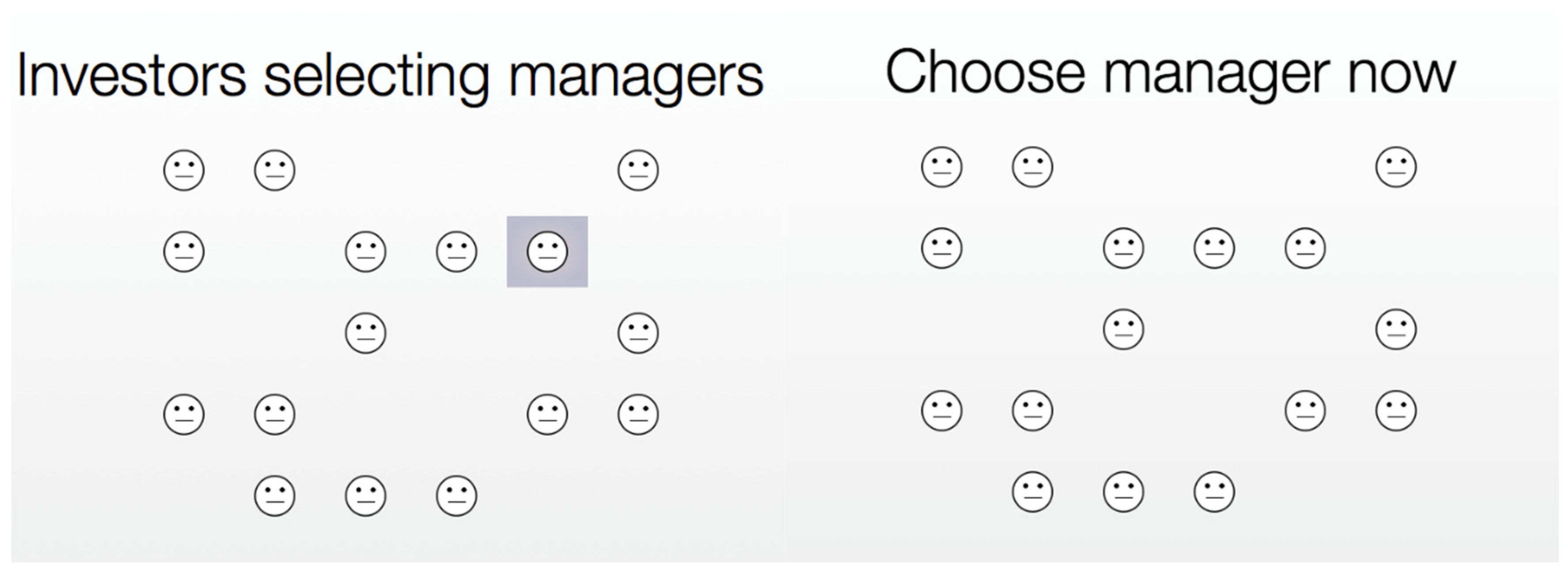
The project managers that are chosen to be employed then choose whether to transfer the extra 10 ECU or not, as illustrated by the screenshots below.
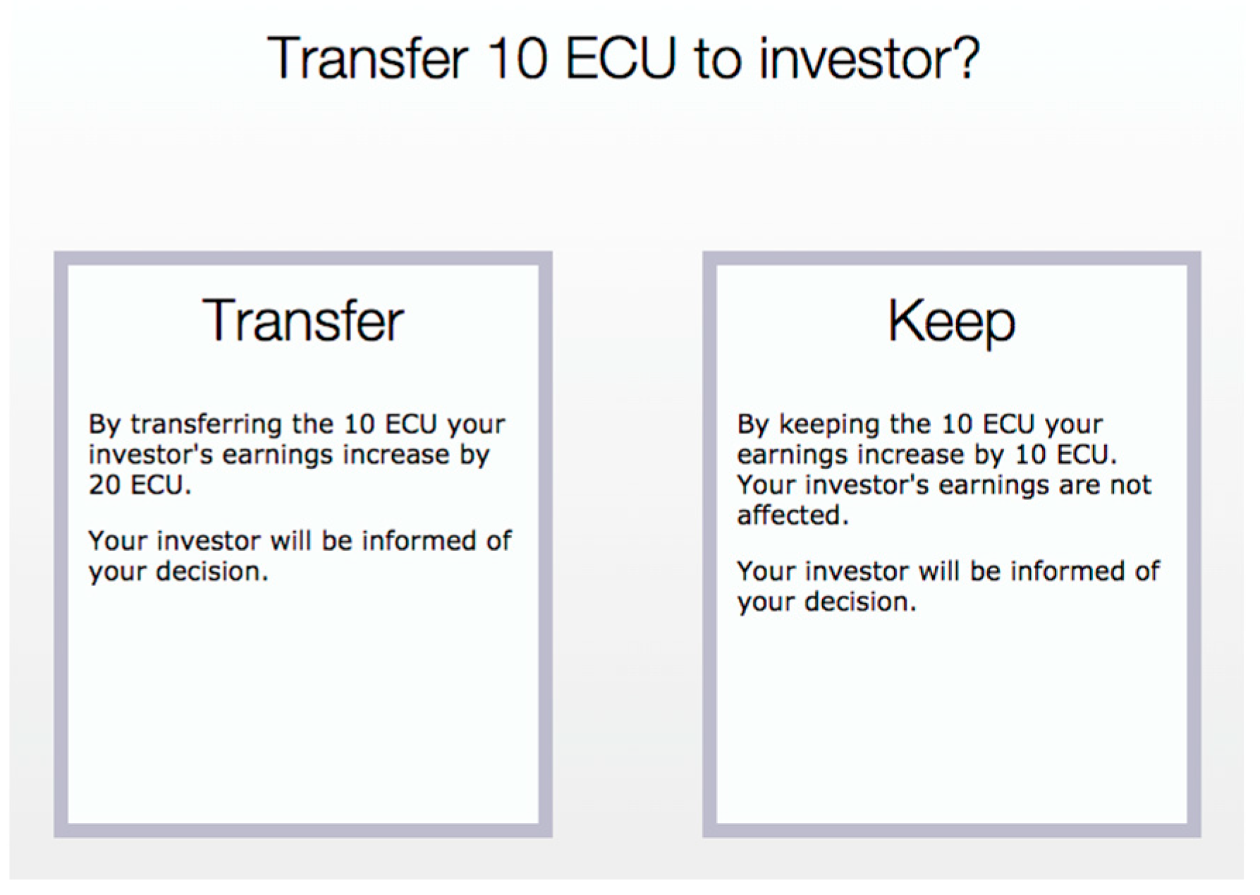
After deciding to transfer or not, the employed managers choose a project from a screen with eight different projects, as illustrated in the left screenshot below. They do so in the same order in which they were chosen to be managers. Half of the projects are of the type that is more likely to be successful and the other half is of the type that is less likely to be successful, but which is which is unknown at the time of choice. Once all employed managers have chosen a project, the manager implements the project by clicking on the box in the right screenshot. Investors and employed project managers are then told whether their own project was a success or a failure.
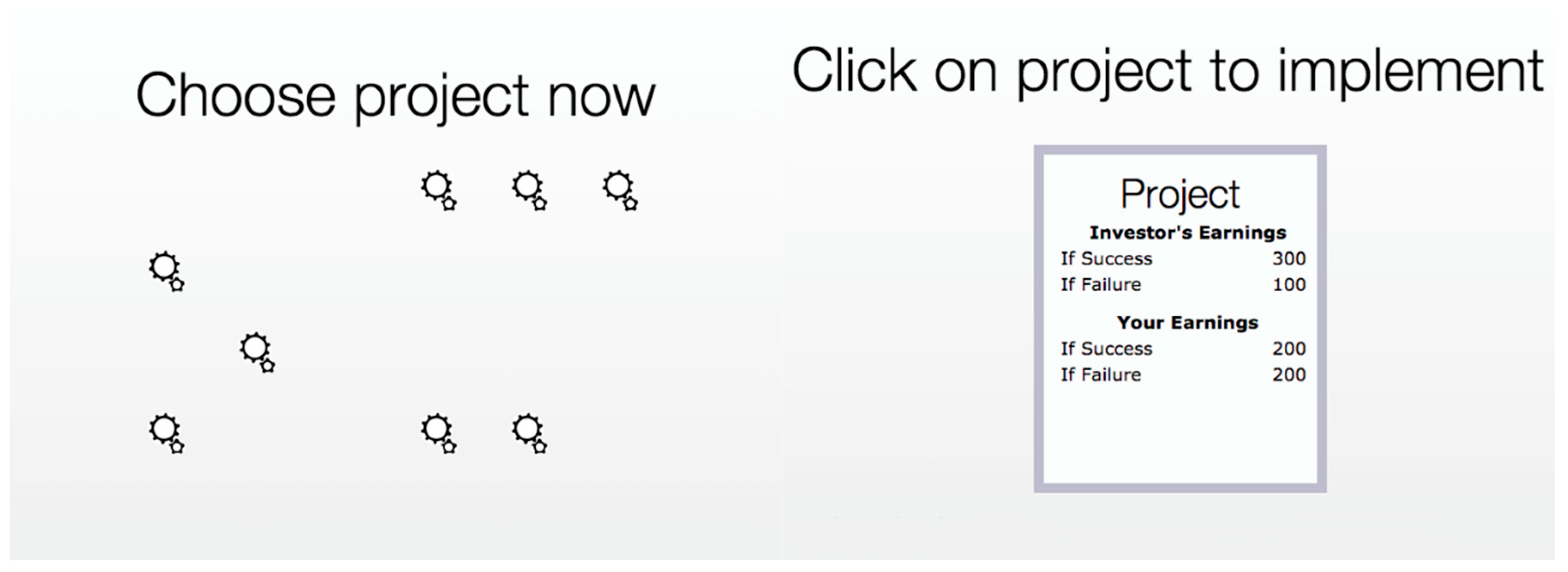
- The Second Project
Finally, a second project is to be implemented. However, in this case the situation changes: The investor can either proceed with the same currently employed manager or choose a new project manager.
If the investor chooses to go on employing the current project manager, the first project is going to be implemented once more. It will still have the same success probability as before, meaning that if the project manager selected a project with a high success probability of 75% it still has that success probability of 75%, and similarly for a project with a low success probability of 25%.
Of course, a previously successful project need not necessarily have to be of the high success probability type, and an unsuccessful project need not necessarily have to be of the low success probability type.
If, instead, the investor chooses to change to a new project manager, this manager will then choose from a set of 8 new projects. These projects are again equally likely to be of the high (75%) or low (25%) success probability type.
Note that new projects can have different earnings, both if successful or unsuccessful. The investor will be informed about the new earnings before choosing whether to stay with the current project and project manager or switching to a new one.
A new project manager is chosen on a screen similar to the first time that a manager was chosen. Note, furthermore, that none of the managers that the investor can choose from at that stage have been chosen for a project before. This also implies that a manager who was employed for a first project, but who gets replaced by a new manager, will not be employed for a second project.
- Earnings from Projects
Investors: for the first project an investor will earn 300 ECU in case of success and 100 in case of failure. The second project can have different earnings.
Project managers: during the first project a project manager will earn 200 ECU, independent of whether the manager has been employed by an investor or not. For the second project only employed managers will again earn 200 ECU. Those who are not employed for this project earn nothing.
Here is an example of the screen that the investor may see when making her decision for the second project:
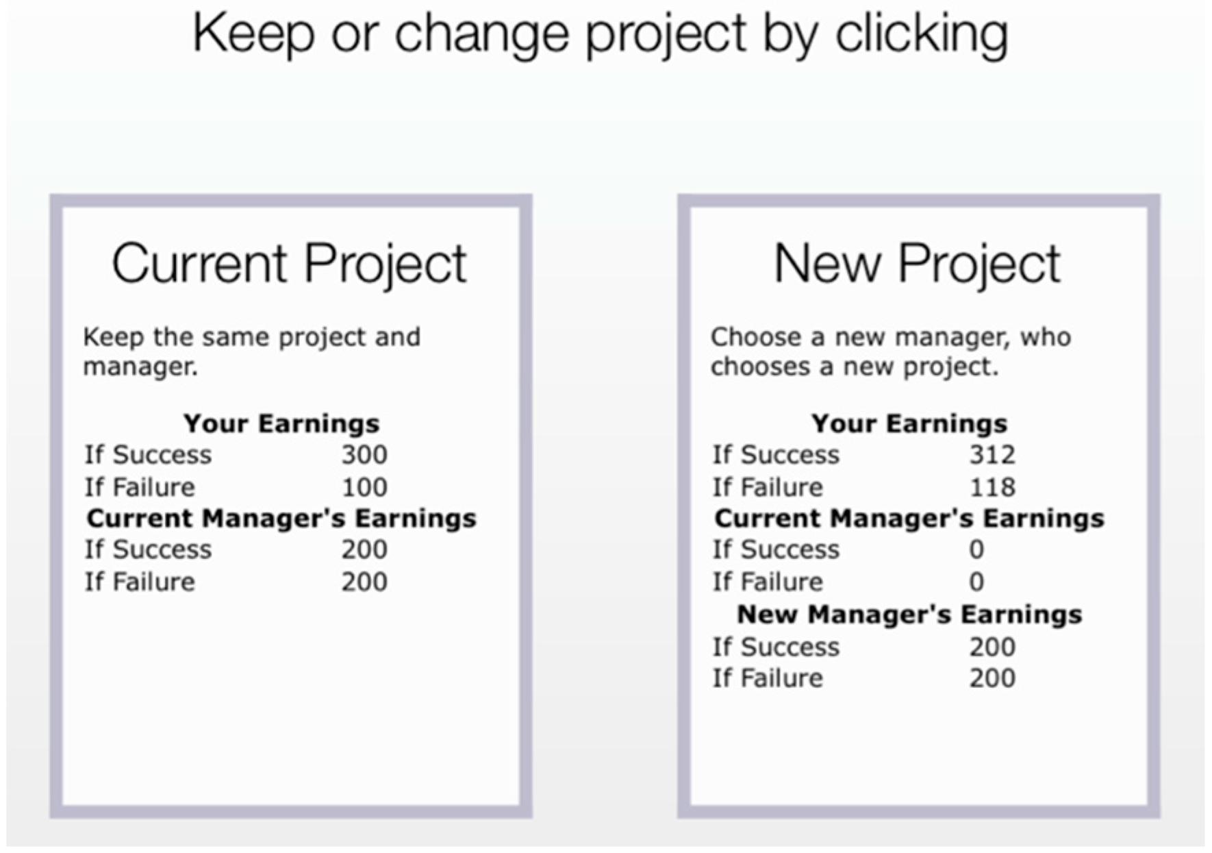
- Summary
- In this experiment you are either an investor or a project manager.
- The experiment consists of eight different rounds.
- In each round, each investor chooses a project manager, who then decides whether to transfer 10 ECU to increase the investor’s earnings by 20 ECU, or to keep the 10 ECU.
- Next, these employed managers choose a project that either succeeds or fails with a certain probability.
- For the second and final project in a round, an investor can decide either to stay with the current project and manager, or have a new manager choose a new project.
- For the first project an investor will earn 300 ECU in case of success and 100 ECU in case of failure. The second project can have different earnings.
- A manager earns 200 ECU for the first project, even if not employed. For the second project a manager earns 200 ECU if employed, and 0 ECU if not employed.
- Only one of the eight rounds (with two projects each) will be randomly selected for payment.
Appendix B.2. Questionnaires
Appendix B.2.1. Transfer, Manager
- What is your age (in numbers)?
- What is your gender?
- female
- male
- What is your (primary) study program (if not a student please choose that)?
- How would you describe your decision making process when deciding whether to send a transfer or not?
- Did you send any transfers to your investor after being chosen?
- Yes
- No
- If yes, which was the most important reason to do so?
- Transferring doubled the income for the group as a whole
- I hoped making the transfer would make the investor stay with my project
- I just tried to be nice to the investor
- Were you disappointed by an investor who switched to another project?
- Yes, every time.
- Yes, but only if my project was better than the alternative.
- Yes, but only if I had sent the transfer.
- No, the investor can choose what they want.
- Not applicable, every investor I met stayed with my project.
Appendix B.2.2. History, Manager
- What is your age (in numbers)?
- What is your gender?
- female
- male
- What is your (primary) study program (if not a student please choose that)?
Appendix B.2.3. Transfer, Investor
- What is your age (in numbers)?
- What is your gender?
- female
- male
- What is your (primary) study program (if not a student please choose that)?
- How would you describe your decision making process when choosing whether to stay with a project manager or not in general?
- Did you calculate the success probability of a project?
- Yes
- No
- I tried to, but failed
- Did you try to calculate the expected value of the different projects? (expected value is probability times earnings)
- Yes
- No
- Did you feel a positive emotion towards a manager who sent you a transfer?
- 1—Not at all
- 2
- 3
- 4
- 5—Very strongly
- The first project never succeeded.
- Did you feel a sense of obligation towards a manager who sent you a transfer?
- 1—Not at all
- 2 • 3
- 4
- 5—Very strongly
- Never received a transfer
- Were you more likely to stay with a project and manager if the manager sent you a transfer earlier?
- 1—Not at all
- 2 • 3
- 4
- 5—A lot
- Never received a transfer
Appendix B.2.4. History, Investor
- What is your age (in numbers)?
- What is your gender?
- female
- male
- What is your (primary) study program (if not a student please choose that)?
- How would you describe your decision making process when choosing whether to stay with a project manager or not in general?
- Did you calculate the success probability of a project?
- Yes
- No
- I tried to, but failed
- Did you try to calculate the expected value of the different projects? (expected value is probability times earnings)
- Yes
- No
- Did you feel a positive emotion towards a manager if the first project succeeded?
- 1—Not at all
- 2
- 3
- 4
- 5—Very strongly
- The first project never succeeded
- Did you feel a sense of obligation towards a manager who’s first project was a success?
- 1—Not at all
- 2
- 3
- 4
- 5—Very strongly
- Never received a transfer
- Were you more likely to stay with a project and manager if the manager’s first project was a success and, if so, how much more?
- 1—Not at all
- 2
- 3
- 4
- 5—A lot
- Never received a transfer
Appendix B.2.5. Control, Investor
- What is your age (in numbers)?
- What is your gender?
- female
- male
- What is your (primary) study program (if not a student please choose that)?
- How would you describe your decision making process when choosing whether to stay with a project or not in general?
- Did you calculate the success probability of a project?
- Yes
- No
- I tried to, but failed
- Did you try to calculate the expected value of the different projects? (expected value is probability times earnings)
- Yes
- No
Appendix C. The Role of Other Social Preference Models in Our Design
Looking at History first, given the experimental design, none of the prominent social preference models in economics play a role whatsoever. This is a direct result of two design features. Firstly, managers do not have any influence on the payoff of the investor beyond the act of randomly choosing a project that is more or less likely to be successful. This precludes any influence of reciprocity of any kind. Secondly, the payment scheme chosen for the (active and inactive) managers effectively nullifies inequality concerns that investors might have regarding the effect of their choice on other participants. By the time the investors’ decisions are made, every manager has earned the exact same amount (200 ECU). Motives such as inequity aversion or envy are meaningless. Since investors cannot affect the distribution of earnings in any way, this is true irrespective of the exact theory applied, such as, for example, Fehr and Schmidt (1999) or Bolton and Ockenfels (2000). In fact, social welfare concerns are not germane either, making irrelevant approaches such as altruism (giving the same weight to each anonymous manager), simple max-min preferences or the model of Charness and Rabin (2002).
In Transfer, the situation is somewhat different. Since the transfer decision is intentional, intention-based reciprocity models (Rabin, 1993; Dufwenberg & Kirchsteiger, 2004) or type-dependent preferences (Levine, 1998) are potentially relevant, that is, if kindness is at stake. However, about 90% of the transfers in our experiment are self-reportedly strategically selfish. A similar finding is reported in Malmendier and Schmidt (2017), which is also supported by the observation that gift receivers understand this phenomenon well. These results cast doubt on the relevance of kindness. This may not be surprising as participants typically enroll in an experiment to earn money, and the experimental context in this case focuses attention on the re-appointment or replacement as manager (a self-related context). Moreover, why would an investor bother about the precise motivation of their manager at the time the transfer was sent—which is not immediately preceding their decision as in Malmendier and Schmidt (2017)—given the mental effort it entails (Zhang & Epley, 2012). Inequality-oriented motives, furthermore, clearly play a negligible role. First of all, given the experimental design, they are potentially only relevant if the manager withholds the transfer and; in addition, earnings are individually considered (not averaged as in Bolton and Ockenfels (2000)). Moreover, in that case, the manager earns 10 ECU more than managers who did not send the transfer or, more importantly, were inactive, which amounts to only one-twentieth of their fixed payoff, if selected for the final project.
Notes
| 1 | For more extensive reviews, see: Malmendier and Schmidt (2017), Maréchal and Thöni (2019). |
| 2 | In this context, they refer to the prominent sociologists Gouldner (1960) and Blau (1964) arguing that the obligation to reciprocate is a universal social norm. |
| 3 | A third module of ATM concerns a generalization of tie values, based on previous interaction experiences, towards novel interaction partners in similar environments, called a generalized tie value (van Winden, 2023). This module will be neglected here, due to a lack of data. |
| 4 | See Malmendier and Schmidt (2017, pp. 506–507) for evidence. |
| 5 | There is also evidence that neurological processes related to preference ordering are activated when cues are not consciously recognizable (Pessiglione et al., 2008), and that subjects may unconsciously learn how to perform a task (Lebreton et al., 2009). |
| 6 | Note that the investor has no fixed payment but is the residual claimant (cf. Bandiera et al., 2009). |
| 7 | To ensure attention, inactive managers are given the possibility to watch a neutral video while they are inactive. Any behavioral effects of the video are irrelevant since we do not analyze the managers’ behavior. |
| 8 | The size of the transfer is chosen based on the observation that in the Malmendier and Schmidt (2017) experiment a transfer (gift) that is similarly sized relative to a project’s expected earnings leads to a reasonably even distribution of transfer and no transfer decisions. |
| 9 | This is intended to minimize the scope for inequity aversion as much as possible in the experiment. |
| 10 | In the instructions to Control and History participants are told a second time that information from earlier draws can be used to estimate the success probability of a project, on top of merely outlining the design of the experiment. This is not the case in Transfer. |
| 11 | Inactive managers were not compensated for the transfer stage. Therefore, active managers that had not sent the transfer had a slightly higher payoff than inactive managers. |
| 12 | The hypothesis of equal transfer ratios in all rounds is rejected at a 5%-significance level due to one outlier in round 3, where 90% of all transfers are sent. Excluding that round, the hypothesis cannot be rejected (Chi-square p = 0.695). Regressing the transfer decision on a trend in a random effects model produces a significantly negative coefficient at the 5% level (see Figure A1 in Appendix A). |
| 13 | The null hypothesis of equal project switching rates in the different rounds cannot be rejected (p = 0.66) and there is no discernible trend. |
| 14 | p = 0.069 in a regression of only the trend and a constant in a random effects model. |
| 15 | Unless otherwise specified, we use logit regressions with standard errors clustered at the subject level to test for significance when comparing switching rates. While the subjects interact indirectly, we argue that there is no possible channel for behavioral spillover within a group of investors, allowing us to treat different investors as independent. We also ran a test on only the first round as a robustness check, but results are only reported if they differ qualitatively using common significance criteria. |
| 16 | The lowest p-value occurs comparing Control and Transfer at p = 0.227. |
| 17 | In this case, the data are insufficient to run a meaningful test using only the first round. |
| 18 | Predicted between-treatment-change in the difference of switching probabilities relative to experience, keeping all other variables at their mean and using specification (4) from Table 2: Control vs. History 3.9%, p = 0.64; Control vs. Transfer: 23.5%, p < 0.01. |
| 19 | In line with Malmendier and Schmidt (2017) no effect of gender and field of study is observed. See Appendix A Table A3 for the same regression using a probit model. Results are qualitatively the same. |
| 20 | Using a clustered t-test, both comparisons of Control vs. History and Control vs. Transfer investor decision times have p-values below 0.001, while the difference between History and Transfer is not significant. Regarding investor decisions, decision time comparisons were also conducted on only the first round as a robustness check (using a simple logit instead of a random effects panel model); however, results are only reported if they differ qualitatively, as per common significance criteria. Note that all decision times include the 3 s that an investor must wait as part of the confirmation screen, plus additional waiting time if they decide to change their decision before confirming. In History and Transfer subjects, an additional reminder of the effect a decision has on managers is provided, but this is identical in all 8 rounds and hence unlikely to be relevant for this comparison. |
| 21 | Note from Appendix A Figure A4 that in both social treatments, after a positive experience, the decision time for staying with the current manager is longer than for decisions to switch, a relationship that completely reverses after a negative experience, whereas no reversal is observed in Control (difference between stay and switch in Control: from +0.2 to +0.2; in History: from +2.6 to −2.1 s; in Transfer: from +2 to −4.8 s). The differences only become weakly significant in a regression using an experience/investor decision dummy when pooling the social treatments, but not when analyzed in isolation for any individual treatment. |
| 22 | See Appendix B.2 for the exact questions. Note that, due to a coding error, the final answer should have been “The first project never succeeded” in the History treatment but was shown as “Never received a transfer.” This was not noticed by any subjects during the experiment. |
| 23 | Emotion and obligation feelings are only weakly correlated in Transfer (0.35, p = 0.06). See Table A5 for a full overview. |
| 24 | Running the same regressions separately for History and Transfer mostly results in results too weak to make conclusive statements about the directionality of the effect, except for likely to stay, the coefficient of which is a negative and significant (p = 0.03), when interacted with positive experience in Transfer. |
| 25 | Consistent with our argumentation, adding the interaction term “Obligation x Transfer” shows an insignificant effect of obligation in Transfer, while leaving the other estimates qualitatively the same. |
| 26 | According to van Winden (2023) the internalization of a social norm requires an already existing positive bond with the norm instiller(s). |
| 27 | This contrasts with Malmendier & Schmidt’s view (see Introduction) that a gift triggers an obligation to repay, which follows a universal internalized social norm. More on this in the Concluding Discussion. |
| 28 | To put the impact of a transfer into further perspective, note that its effect on the investor’s earnings is much less dramatic, compared to the potential gains in the other two treatments. While a successful project outcome implied a gain of 200 ECU relative to a project failure, a transfer only earned 20 ECU. |
| 29 | For a related discussion in social psychology concerning the conditions for the reduction of prejudice through intergroup contact (contact hypothesis), see (Paluck et al., 2019). |
References
- Abbink, K. (2004). Staff rotation as an anti-corruption policy: An experimental study. European Journal of Political Economy, 20(4), 887–906. [Google Scholar] [CrossRef]
- Andreoni, J., & Miller, J. (2002). Giving according to GARP: An experimental test of the consistency of preferences for altruism. Econometrica, 70(2), 737–753. [Google Scholar] [CrossRef]
- Au, W. T., & Kwong, Y. Y. (2004). Measurements and effects of social-value orientation in social dilemmas: A review. In R. Suleiman, D. V. Budescu, I. Fischer, & D. M. Messick (Eds.), Contemporary research on social dilemmas (pp. 71–98). Cambridge University Press. [Google Scholar]
- Bandiera, O., Barankay, I., & Rasul, I. (2009). Social connections and incentives in the workplace: Evidence from personnel data. Econometrica, 77(4), 1047–1094. [Google Scholar] [CrossRef]
- Bault, N., Fahrenfort, J. J., Pelloux, B., Ridderinkhof, K. R., & van Winden, F. (2017). An affective social tie mechanism: Theory, evidence, and implications. Journal of Economic Psychology, 61, 152–175. [Google Scholar] [CrossRef]
- Berg, J., Dickhaut, J., & McCabe, K. (1995). Trust, reciprocity, and social history. Games and economic behavior, 10(1), 122–142. [Google Scholar] [CrossRef]
- Blau, P. (1964). Exchange and power in social life. Wiley. [Google Scholar]
- Bogaert, S., Boone, C., & Declerck, C. (2008). Social value orientation and cooperation in social dilemmas: A review and conceptual model. British Journal of Social Psychology, 47, 453–480. [Google Scholar] [CrossRef] [PubMed]
- Bolton, G. E., & Ockenfels, A. (2000). ERC: A theory of equity, reciprocity, and competition. American Economic Review, 90(1), 166–193. [Google Scholar] [CrossRef]
- Boot, A. W. (2000). Relationship banking: What do we know? Journal of Financial Intermediation, 9(1), 7–25. [Google Scholar] [CrossRef]
- Brown, M., & Zehnder, C. (2007). Credit reporting, relationship banking, and loan repayment. Journal of Money, Credit and Banking, 39(8), 1883–1918. [Google Scholar] [CrossRef]
- Camerer, C., Loewenstein, G., & Prelec, D. (2005). Neuroeconomics: How neuroscience can inform economics. Journal of Economic Literature, 43, 9–64. [Google Scholar] [CrossRef]
- Chan, C., & Mogilner, C. (2017). Experiential gifts foster stronger social relationships than material gifts. Journal of Consumer Research, 43(6), 913–931. [Google Scholar] [CrossRef]
- Chao, M., & Fischer, G. (2022). Self-interested giving: The relationship between conditional gifts, charitable donations, and donor self-interestedness. Management Science, 68(6), 4537–4567. [Google Scholar] [CrossRef]
- Charness, G., & Rabin, M. (2002). Understanding social preferences with simple tests. Quarterly Journal of Economics, 117(3), 817–869. [Google Scholar] [CrossRef]
- Cochard, F., Van, P. N., & Willinger, M. (2004). Trusting behavior in a repeated investment game. Journal of Economic Behavior & Organization, 55(1), 31–44. [Google Scholar]
- Cornelissen, G., Dewitte, S., & Warlop, L. (2011). Are social value orientations expressed automatically? Decision making in the dictator game. Personality and Social Psychology Bulletin, 37(8), 1104–1116. [Google Scholar] [CrossRef]
- Cornée, S., & Masclet, D. (2022). Long-term relationships, group lending, and peer monitoring in microfinance: Experimental evidence. Journal of Behavioral and Experimental Economics, 100, 101921. [Google Scholar] [CrossRef]
- Cornée, S., Masclet, D., & Thenet, G. (2012). Credit relationships: Evidence from experiments with real bankers. Journal of Money, Credit and Banking, 44(5), 957–980. [Google Scholar] [CrossRef]
- Duchin, R., & Sosyura, D. (2013). Divisional managers and internal capital markets. The Journal of Finance, 68(2), 387–429. [Google Scholar] [CrossRef]
- Duffy, S., & Smith, J. (2014). Cognitive load in the multi-player prisoner’s dilemma game: Are there brains in games? Journal of Behavioral and Experimental Economics, 51, 47–56. [Google Scholar] [CrossRef]
- Dufwenberg, M., & Kirchsteiger, G. (2004). A theory of sequential reciprocity. Games and Economic Behavior, 47(2), 268–298. [Google Scholar] [CrossRef]
- Fehr, E., Goette, L., & Zehnder, C. (2009). A behavioral account of the labor market: The role of fairness concerns. Annual Review of Economics, 1(1), 355–384. [Google Scholar] [CrossRef]
- Fehr, E., & Schmidt, K. M. (1999). A theory of fairness, competition, and cooperation. Quarterly journal of Economics, 114(3), 817–868. [Google Scholar] [CrossRef]
- Finan, F., & Schechter, L. (2012). Vote-buying and reciprocity. Econometrica, 80(2), 863–881. [Google Scholar]
- Gabbi, G., Giammarino, M., Mathias, M., Monferrà, S., & Sampagnaro, G. (2020). Does face-to-face contact matter? Evidence from loan pricing. The European Journal of Finance, 26(7–8), 820–836. [Google Scholar] [CrossRef]
- Gouldner, A. W. (1960). The norm of reciprocity: A preliminary statement. American Sociological Review, 25(2), 161–178. [Google Scholar] [CrossRef]
- Grech, P. D., & Nax, H. N. (2020). Rational altruism? On preference estimation and dictator game experiments. Games and Economic Behavior, 119, 309–338. [Google Scholar] [CrossRef]
- Gurdal, M. Y., Miller, J. B., & Rustichini, A. (2013). Why blame? Journal of Political Economy, 121(6), 1205–1247. [Google Scholar] [CrossRef]
- Haselmann, R., Schoenherr, D., & Vig, V. (2018). Rent seeking in elite networks. Journal of Political Economy, 126(4), 1638–1690. [Google Scholar] [CrossRef]
- Hoffman, B., & Schraw, G. (2010). Conceptions of efficiency: Applications in learning and problem solving. Educational Psychologist, 45, 1–10. [Google Scholar] [CrossRef]
- Johnson, N. D., & Mislin, A. A. (2011). Trust games: A meta-analysis. Journal of Economic Psychology, 32(5), 865–889. [Google Scholar] [CrossRef]
- Kuhnen, C. M. (2009). Business networks, corporate governance, and contracting in the mutual fund industry. The Journal of Finance, 64(5), 2185–2220. [Google Scholar] [CrossRef]
- Langer, E. (1975). The Illusion of Control. Journal of Personality and Social Psychology, 32(5), 311–328. [Google Scholar] [CrossRef]
- Lebreton, M., Jorge, S., Michel, V., Thirion, B., & Pessiglione, M. (2009). An automatic valuation system in the human brain: Evidence from functional neuroimaging. Neuron, 64(3), 431–439. [Google Scholar] [CrossRef] [PubMed]
- Leight, J., Foarta, D., Pande, R., & Ralston, L. (2020). Value for money? Vote buying and politician accountability. Journal of Public Economics, 190, 104227. [Google Scholar] [CrossRef]
- Levine, D. K. (1998). Modelling altruism and spitefulness in experiments. Review of Economic Dynamics, 1(3), 593–622. [Google Scholar] [CrossRef]
- Lunawat, R. (2013). An experimental investigation of reputation effects of disclosure in an investment/trust game. Journal of Economic Behavior & Organization, 94, 130–144. [Google Scholar]
- Malmendier, U. M., & Schmidt, K. M. (2017). You owe me. American Economic Review, 107(2), 493–526. [Google Scholar] [CrossRef]
- Maréchal, M. A., & Thöni, C. (2019). Hidden persuaders: Do small gifts lubricate business negotiations? Management Science, 65(8), 3877–3888. [Google Scholar] [CrossRef]
- Mauss, M. (1990). The gift: The form and reason for exchange in archaic Societies. Routledge. [Google Scholar]
- Murphy, R. O., Ackermann, K. A., & Handgraaf, M. J. J. (2011). Measuring social value orientation. Journal of Judgment and Decision Making, 6(8), 771–781. [Google Scholar]
- Paluck, E. L., Green, S. A., & Green, D. P. (2019). The contact hypothesis re-evaluated. Behavioural Public Policy, 3(2), 129–158. [Google Scholar] [CrossRef]
- Pan, X., & Xiao, E. (2016). It’s not just the thought that counts: An experimental study on hidden cost of giving. Journal of Public Economics, 138(1), 22–31. [Google Scholar] [CrossRef]
- Pessiglione, M., Petrovic, P., Daunizeau, J., Palminteri, S., Dolan, R. J., & Frith, C. D. (2008). Subliminal instrumental conditioning demonstrated in the human brain. Neuron, 59(4), 561–567. [Google Scholar] [CrossRef] [PubMed]
- Rabin, M. (1993). Incorporating fairness into game theory and economics. The American Economic Review, 83(5), 1281–1302. [Google Scholar]
- Rehbein, O., & Rother, S. (2024). Social connectedness in bank lending. The Review of Financial Studies, hhaf014. [Google Scholar] [CrossRef]
- Schulz, J. F., Fischbacher, U., Thöni, C., & Utikal, V. (2014). Affect and fairness: Dictator games under cognitive load. Journal of Economic Psychology, 41, 77–87. [Google Scholar] [CrossRef]
- Silk, J. B. (2003). Cooperation without counting. The puzzle of friendship. In P. Hammerstein (Ed.), Genetic and cultural evolution of cooperation (pp. 37–54). MIT Press. [Google Scholar]
- Strassmair, C. (2009). Can intentions spoil the kindness of a gift? An experimental study. Available online: https://epub.ub.uni-muenchen.de/10351/ (accessed on 27 February 2025).
- van Dijk, F., & van Winden, F. (1997). Dynamics of social ties and local public good provision. Journal of Public Economics, 64(3), 323–341. [Google Scholar] [CrossRef]
- van Winden, F. (2023). The informational affective tie mechanism: On the role of uncertainty, context, and attention in caring. Journal of Economic Psychology, 97, 102625. [Google Scholar] [CrossRef]
- Wazana, A. (2000). Physicians and the pharmaceutical industry. Journal of the American Medical Association, 283(3), 373–380. [Google Scholar] [CrossRef] [PubMed]
- Zajonc, R. B. (2001). Mere exposure: A gateway to the subliminal. Current Directions in Psychological Science, 10(6), 224–228. [Google Scholar] [CrossRef]
- Zhang, Y., & Epley, N. (2012). Exaggerated, mispredicted, and misplaced: When “it’s the thought that counts” in gift exchanges. Journal of Experimental Psychology: General, 141(4), 667–681. [Google Scholar] [CrossRef]
Disclaimer/Publisher’s Note: The statements, opinions and data contained in all publications are solely those of the individual author(s) and contributor(s) and not of MDPI and/or the editor(s). MDPI and/or the editor(s) disclaim responsibility for any injury to people or property resulting from any ideas, methods, instructions or products referred to in the content. |
© 2025 by the authors. Licensee MDPI, Basel, Switzerland. This article is an open access article distributed under the terms and conditions of the Creative Commons Attribution (CC BY) license (https://creativecommons.org/licenses/by/4.0/).