Abstract
We study a simple model in which two vertically differentiated firms compete in prices and mass advertising on an initially uninformed market. Consumers differ in their preference for quality. There is an upper bound on prices since consumers cannot spend more on the good than a fixed amount (say, their income). Depending on this income and on the ratio between the advertising cost and quality differential (relative advertising cost), either there is no equilibrium in pure strategies or there exists one of the following three types: (1) an interior equilibrium, where both firms have positive natural markets and charge prices lower than the consumer’s income; (2) a constrained interior equilibrium, where both firms have positive natural markets, and the high-quality firm charges the consumer’s income or (3) a corner equilibrium, where the low-quality firm has no natural market selling only to uninformed customers. We show that no corner equilibrium exists in which the high-quality firm would have a null natural market. At an equilibrium (whenever there exists one), the high-quality firm always advertises more, charges a higher price and makes a higher profit than the low-quality one. As the relative advertising cost goes to infinity, prices become equal and the advertising intensities converge to zero as well as the profits. Finally, the advertising intensities are, at least globally, increasing with the quality differential. Finally, in all cases, as the advertising parameter cost increases unboundedly, both prices converge increasingly towards the consumer’s income.
JEL Classification:
D83; L13; M37
1. Introduction
The global advertising and communication market today weighs more than 1370 billion dollars (i.e., approximately 1.5 per cent of global GDP, in 2019) and continues growing faster than the world GDP. Advertising appears to be a key factor in the competition between firms. In France, for instance, commercial communication “expenditure”, strictly speaking (excluding human resources in particular), weighs 31 billion, which is nearly the equivalent of private investment in R&D (32 billion).
The question of differentiation and quality is a natural part of the debate. Advertising has been studied mainly in the case of horizontally differentiated markets. Only a few papers deal with the case of advertising in vertically differentiated markets, leaving important questions pending. We aim at filling the gap by studying random (or mass) advertising in a vertical differentiation model with a price competition. We aim at determining whether the advertisement increases with the quality sold and whether an increase in the advertising cost has a differential or a similar impact on the firms’ prices, advertising intensities and profits.
Advertising is generally considered either as persuasive or informative. In the first case, it does not provide any actual information on the product but tries to appeal to consumers’ desires and drives to have them buy the good. In the second one, it provides information on the existence of the product, the price, the characteristics of the good and so on. Advertising is also often considered as a quality signal if higher quality products are more advertised than lower quality ones, in which case it is indirectly informative.
In this paper, we deal directly with informative advertising in the framework of an oligopolistic competition. We analyze a simple vertical differentiation duopoly model with a low-quality firm and a high-quality one, where consumers differ in their preference for quality. The consumers are initially uninformed of the existence of the firms. When receiving an ad from one firm, they learn its existence, its price and its product quality.1 We focus on random (or mass) advertising, i.e., the dissemination of promotional content without any targeting of consumers. Each firm chooses its price and its advertising intensity (which, here, amounts to choosing a rate of the consumers population to be informed uniformly). We assume that consumers cannot spend on the good more than their (identical) income (or, possibly, a predetermined share of it), which puts an-upper bound on prices.2
We consider a vertical differentiation model, i.e., where consumers are unanimous on the ranking of variants sold at the same price (as considered in many papers, such as Gabszewicz and Thisse, 1980 [1]; Shaked and Sutton, 1982 [2], among others).3 Consumers differ, nevertheless, with regards to the intrinsic characteristic that we call an “intensity of preference for quality”, which measures how strongly a consumer is sensitive to quality, and thus how much a priori s/he is willing to pay to acquire a better quality. Moreover, we suppose consumers to be limited by a budget constraint, or, equivalently, that prices are upper-bounded by an exogenous limit. In doing so, we are supposing that the heterogeneity in the intensity of a preference for quality is not equivalent to the heterogeneity in income. The abundant literature in marketing and psychology may find this hypothesis by mainly using motivation theory (Reeve, 2017) [4]. Any purchase occurs, as any behavior, to satisfy physical (hunger; thirst) or psychological needs (recognition; esteem; belonging). When the need is activated, the consumer experiences a state of tension, driving the consumer to try to satisfy the need. The strength of the tension determines the intensity with which the individual is going to seek for the satisfaction of his/her need. Suppose the quality refers to environmental attributes, i.e., it measures the effort made by the firm to respect the environment in the entire process. Consumers differing in terms of individual and familial histories, physical and intellectual capabilities, cultural backgrounds, reaction and sensitivity to marketing4 would necessarily differ intrinsically with regards to the efforts they are willing to make to be friendly to the environment, possibly independently from their budget constraint or income. The intensity of the preference for quality ( in the model), representing the motives we have just described, is different in nature from the income (y), which represents what extrinsically limits the expenses. Considering both in the same model gives rise to interesting results that we would not have been able to observe, had we considered only one of them.
First, we characterize the firms’ choices at equilibrium. We show that, depending on the consumer’s income and the ratio between the advertising cost and quality differential (relative advertising cost), either there is no equilibrium in pure strategies or, one of three possible types of equilibrium holds. (1) Interior Equilibrium (IE), where both firms have positive “natural markets”5 and charge prices lower than the consumer’s income; (2) constrained Interior Equilibrium (CIE), where both firms have positive natural markets and the high-quality firm charges the consumer’s income; (3) corner equilibrium (COR), where the low-quality firm has no natural market. The intuition is that if there is no upper-bound or if the upper-bound on prices is too high, at least one among the two firms may benefit from deviating from the candidate equilibrium to a higher price and serving the customers who are uninformed of the existence of its rival. The necessity for the existence of an interior equilibrium of an upper-limit on prices is a first contribution to the existing literature. Once this upper limit is introduced, it plays an explicit role in the existence and the nature of the equilibrium, i.e., in particular, it entails the possible existence of a corner equilibrium and of a constrained interior equilibrium. This is a second contribution of this paper. All of these features have indeed been overlooked in the literature (see, for instance, Grossman and Shapiro, 1984 [6]; Tirole, 1988 [7]) which correspond to a specific contribution of this paper.
Secondly, we provide several comparative statics results at equilibrium, studying how the outcome at equilibrium varies with the relative advertising cost, for some given the consumer’s income. Depending on this income, when this relative advertising cost varies, we may go through two or three regimes, and even go through a hole (with no equilibrium). Interestingly, contrary to what has been supposed by the existing literature that considered only the interior equilibrium overlooking the problem of existence and the possible existence of equilibria of different types, the equilibrium may never be an interior one (for sufficiently low consumers’ income). For sufficiently high consumers’ income, the equilibrium is an interior equilibrium for low enough values of the relative advertising cost, but the type of equilibrium necessarily changes as the relative advertising cost goes beyond some threshold; and for still higher consumers’ income, we may come up against an existence problem. Moreover, the higher the consumer’s income, the larger the segment of the relative advertising cost for which there is no equilibrium. Hence, looking for all the possible types of equilibrium and investigating the existence problem properly, are not superfluous mathematical exercises.
Very intuitively, prices are increasing (in a broad sense) with the relative advertising cost. Beyond some critical threshold of this relative cost, both prices become equal to the consumer’s income.
Concerning the advertising intensities, both are decreasing (in a broad sense) in the cases of intermediate and high consumers’ income, as it can be predicted intuitively. But, in the case of low consumers’ income, the advertising intensity of the low-quality firm is increasing on a range of intermediate levels of the relative cost.
Regarding the profits, both go through three phases (not synchronized): they are decreasing at Phase 1, increasing at Phase 2 and then decreasing at Phase 3, converging each to zero as the ratio goes to infinity.
As for the profits ratio, equal to the high-quality firm’s profit over the low-quality firm’s one, it is always larger than 1, meaning that it always pays to be the high-quality firm. The variation of this ratio is, however, not simple. It goes through an increasing phase for a range of relative advertising costs close to zero, and it is decreasing for sufficiently high levels of this relative cost, converging to 1, as the relative cost advertising goes to infinity, meaning that it pays less and less to be the high-quality firm, as the relative cost increases unboundedly.
Literature Review
There is important literature in this field originating with the works of Butters (1977) [8], in the case of homogeneous goods (see, also, the more recent contribution of Roy, 2000 [9]). Grossman and Shapiro (1984) [6] and Tirole (1988) [7] launched the basis for the case of horizontally differentiated markets, distinguishing between mass (random) advertising (where there is no correlation between advertising intensities and consumers’ types) and targeted advertising (when the firms advertise their more interesting consumers more frequently). More recent papers consider the question of advertising within the horizontal differentiation framework, such as Celik (2007) [10], Ben Elhadj-Ben Brahim et al. (2011) [11] and Esteban and Hernandez (2014) [12]. Simbanegavi (2009) [13] also considers advertising within a horizontally differentiated market, but deals with the different question of cooperation between the firms on advertising or prices. The horizontal differentiation papers generally deal with ex ante symmetric firms, contrary to vertical differentiation ones.
A strand of literature considers questions relative to advertising targeting, supposing an exogenous segmentation of consumers: Esteves and Resende (2016, 2019) [14,15]; Iyer et al. (2005) [16]; Esteban and Hernandez (2016) [17]; Zhang and He (2019) [18]; Zhang, Cao and Yue (2018) [19]; Galeotti and Moraga-Gonzalez (2003) [20]. Even if the models in the cited papers may reflect some differentiation, to the extent that consumers do not react in the same way to a price differential between firms, it is definitely not vertical differentiation, as there is no unanimity on the ranking of the products by well-informed consumers.
Concerning asymmetry, all these papers consider symmetric firms except Zhang and He (2019) [18], who consider the exogenous cost asymmetry between firms, while in our model, this asymmetry is inherent to the vertical differentiation; the cost asymmetry emerges endogenously through the asymmetry in the choice of firms in terms of advertising intensities.
Colombo and Lambertini (2003) [21] is one of the few papers we identified that deals with advertising in a vertically differentiated market. But, our work is different in several respects. First, they consider persuasive advertising, while advertising is informative in our paper. Second, they deal with the endogenous interplay between advertising and product quality, while we consider exogenous qualities. Third, they consider a vertical differentiation model different from the one we consider. Tremblay and Martin-Filho (2001) [22] and Tremblay and Polasky (2002) [23] consider advertising within a vertically differentiated market but with persuasive advertising. Elliott (2004) [24], Esteban and Hernandez (2007) [25] Esteban and Hernandez (2018) [26] consider a vertical differentiation model but consider mass advertising as the distribution of ads to the entire market with no choice of advertising intensities.
Loosely related to our paper, Shen and Villas-Boas (2018) [27] deal with behavioral-based advertising, but, the valuation of consumers of the product in the second period, in the case of monopoly in a two-period model, may be correlated with her valuation in the first period. Johnson (2013) [28] deals with targeting within a model, where a continuum of firms choose the advertising amount, while consumers have the possibility to block ads, with no competition among firms.
This paper is organized as follows. Section 2 describes the model. Section 3 provides the results. Section 4 provides some comparative statics. Section 5 concludes.
All proofs are given in Appendix B.
2. The Model
Two firms produce two vertically differentiated products with exogenous qualities. Firms 1 and 2 are, respectively, the high- and the low-quality firm. The quality differential is denoted by We assume that marginal costs are zero and that Firms 1 and 2 compete in uniform prices, respectively, and . Firms invest in advertising to inform consumers about their existence, products’ characteristics and prices.
No production cost is supposed, for simplicities’ sake. It would be natural to suppose asymmetric costs with a higher cost for the high-quality firm. We were compelled to such a simplification, which already resulted in tough calculations. Moreover, cost asymmetry arises endogenously. Indeed, we will prove that, at equilibrium, the higher quality firm spends more on advertising than the lower quality one. This amounts somehow to an endogenous fixed cost (relative to quantities) that is proved to be higher for a higher quality.
There is a unit mass of consumers. Consumers are initially totally unaware of the existence of the firms and may become informed only through advertisements.6 Consumers informed only of the existence of Firm i buy one unit of i’s good, provided that its price is not greater than their income Y. Consumers informed of the existence of both firms buy the product which better fits their needs.7 A type -customer derives a gross utility from consuming one unit of the quality i-good in a given period, hence the indirect utility . Characteristic is uniformly distributed over , with a density normalized to 1.
The prices are thus assumed to belong to . U is assumed to satisfy , so that all consumers who are aware of the existence of at least one firm buy the good.
We define as the marginal consumer, i.e., the consumer who, when informed of the existence of both firms, is indifferent between purchasing at Firm 1 or at Firm 2. That is:
When fully informed, consumers with types greater than buy from Firm 1, while consumers of types smaller than buy from Firm From now on, we call Firm 1’s “natural market” and Firm 2’s “natural market”. When , Firm 2’s natural market is the whole market, and Firm 1 has a null natural market share. When both firms have a strictly positive natural market share. When Firm 1’s natural market is the whole market, and Firm 2 has a null natural market.
We consider here the case of mass or random advertising, in which the advertising intensity of Firm i, i.e., the proportion of consumers who are informed about product i, is uniform over all consumers’ types. This means that a fraction of consumers are informed of the existence of both firms (thus, they may actually compare between both and choose the one that ensures the best utility, as in the standard literature), a fraction are informed of the existence of none of them (thus, they buy nothing), a fraction are only informed of the existence of Firm 1 (and buy from it) and a fraction are only informed of the existence of Firm 1 (and buy from it). The cost of reaching a fraction of type -consumers is simply
For convenience, we define the relative prices , the relative income and the relative cost .
The game: the firms choose simultaneously8 prices in (or, equivalently, the relative prices in ) and advertising intensities .
3. The Equilibrium Outcomes
At the equilibrium, whenever there exists any, three cases are possible. (1) The two firms have positive natural markets and charge prices lower than the consumer’s revenue (interior equilibrium); (2) the two firms have positive natural markets with the high-quality firm charging a price equal to the consumer’s revenue (constrained interior equilibrium); (3) only one of the firms has a positive natural market (corner equilibrium). When no equilibrium candidate among the three described is an equilibrium, the game admits no pure-strategy equilibrium.
From the definitions, the profits of the two firms are, respectively:
The profits are thus defined above in the three possible price configurations: (i) When Firm 1 has no natural market and sells only to consumers unaware of the existence of its rival but informed of its own existence, while Firm 2 can sell to all customers informed of its existence; (ii) both firms have a positive natural market, and it sells both to consumers in their natural market and to consumers unaware of the existence of their rival, provided they are informed of their existence; (iii) if , Firm 2 has no natural market and sells only to consumers unaware of the existence of its rival but informed of its own existence while Firm 1 can sell to all customers informed of its existence. We define the relative profits to be
A pure-strategy Nash equilibrium of this game is a quadruple , such that is the best reply to for each , and . Proposition 1 characterizes the equilibrium whenever it exists in the space , and Figure 1 pictures, in this space, the areas corresponding to the different types of equilibria and to the nonexistence of a pure-strategy equilibrium.
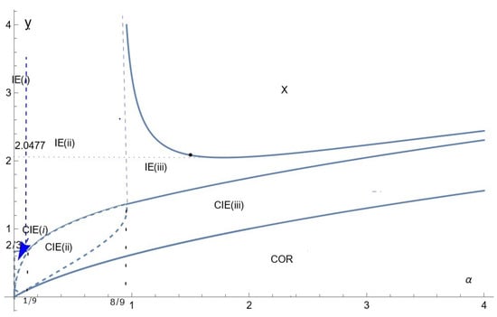
Figure 1.
Equilibrium in the -space.
Proposition 1
(Equilibrium). Whenever an equilibrium exists, it is unique. Depending on the position of relative to the zones depicted in Figure 1 and defined analytically in Appendix A, there are four main cases in terms of the existence and type of equilibrium.
- 1
- Zone IE (interior equilibrium): both firms have positive natural markets and charge prices lower than the revenue of the consumers. This zone is divided into three sub-zones, depending on whether or not the firms reach all consumers.
- IE(i)
- Both firms reach all consumers (), and relative prices are
- IE(ii)
- The high-quality firm reaches all consumers, while the low-quality firm reaches only a fraction of them: , ; the equilibrium relative prices are:
- IE(iii)
- Both firms reach only a fraction of consumers.9
- 2
- Zone CIE (constrained interior equilibrium): Both firms have positive natural markets, but the high-quality firm charges the revenue of consumers. This zone is also divided into three sub-zones, depending on whether or not firms reach all consumers.
- CIE(i)
- Both firms reach all consumers: , and charge the relative prices
- CIE(ii)
- The high-quality firm reaches all customers (), the low-quality firm only a fraction of them and relative prices are given by: ,
- CIE(iii)
- Both firms reach only a fraction of customers; the high-quality firm charges the relative price and the low-quality firm charges a lower price.10
- 3
- Zone COR (CORner equilibrium): the low-quality firm has a zero natural market, with the following relative prices and advertising intensities:
- 4
- Zone X: There is no equilibrium in pure strategies.
From Figure 1, it appears clear that a pure strategy equilibrium exists whatever the value of y when the relative advertising cost is small enough (smaller than 8/9). The question why is quite clear. When the advertising cost is small and/or the quality differential is high, Firm 1 informs all customers, which leaves no possibility for Firm 2 to serve uninformed consumers at a high price. Another feature is that the range of values of y for which an interior equilibrium11 exists shrinks when the relative advertising cost increases. This is because, as this relative cost increases, less and less consumers are informed; thus, a deviation toward serving at a high price only becomes more and more profitable, because consumers are unaware of the existence of one’s rival, and this prevents the equilibrium candidate from being an equilibrium.
To prove Proposition 1, we deal consecutively with each possible case.
For the first case (interior equilibrium), we write the first-order conditions for the associated Lagrangian, supposing that each firm has a positive natural market. After eliminating the trivial solution with null prices and advertising rates, we examine the four possible cases: (i) Both firms reach all customers (); (ii) Firm 1 reaches all customers, but Firm 2 only reaches a fraction of them (, ); (iii) both firms reach only a fraction of their customers (, ); (iv) Firm 1 reaches only a fraction of its customers, and Firm 2 reaches its whole natural market (, ).
For sub-cases (i), (ii) and (iii), we calculate the equilibrium candidates and determine necessary and sufficient conditions for each candidate to correspond to a maximum for the set of prices, such that both firms have positive natural markets. As for case (iv), it turns out that it can never correspond to an equilibrium.
The reasoning above eliminates the deviations such that each firm has a positive natural market, but not deviations such that one of them has no natural market. Look at the profit of Firm i when it has no natural market share and its competitor does not reach the entire market (). We see easily that this profit may increase unboundedly with the price, and hence may become higher than the profit at the equilibrium candidate, thus constituting a profitable deviation. Therefore, if the upper-bound on prices is too high, the equilibrium candidate cannot be an equilibrium. In other words, to ensure that the identified candidate is an equilibrium, the price must not be allowed to be too high, so that the best possible deviation is not profitable. In each sub-case of case 1) of Proposition 1, we write conditions of y and , such that, on the one hand, the profit at the best possible deviation is lower than the profit at the equilibrium candidate; and on the other hand, the price candidates are less than Y.
Regarding case 2 (constrained interior equilibrium), we proceed exactly in the same way as for case 1, except that we take the constraint on prices into account in the Lagrangian.
As for case 3 (corner equilibrium), we identify the corner equilibrium in each considered situation (either Firm 1 or Firm 2 has a null natural market). Then, we consider possible deviations.
There is an asymmetry between firms regarding the existence of corner equilibria. While a corner equilibrium with a null natural market for the low-quality firm may exist, there is never an equilibrium with a null natural market for the high-quality firm. Indeed, the low-quality firm is the one which has less incentives to have customers who would buy the product when they know its “true value”. Thus, it may be interested in relying completely on uninformed customers.
4. Comparative Statics
We are now going to provide some comparative statics at the equilibrium whenever it exists. There are qualitatively three cases depending on the position of the consumer’s income relative to the two critical values (2/3 and approximately 2.0477), as depicted in Figure 1. We refer to the three cases as low, intermediate and high consumer income, which is self-explanatory. We are going to study, in the three cases, consecutively, the prices/advertising intensities, profits and profits’ ratio (the high-quality firm’s profit over the low-quality firm’s profit), as a function of , the relative advertising cost. This amounts to moving along a horizontal line in Figure 1. In doing so, we may go through multiple regions characterized by different types of an equilibrium. For instance, for , increasing starting from zero, we go through CIE (i), then CIE (ii), then CIE (iii) and finally COR and remain there.
Corollary 1 provides the comparative statics for prices and advertising intensities. Figure 2, Figure 3 and Figure 4 depict the relative equilibrium prices as a function of the relative advertising cost, respectively, in the low, intermediate and high consumers’ income. Figure 5, Figure 6 and Figure 7 depict the equilibrium advertising intensities as a function of the relative advertising cost, respectively, in the three cases and in the same order.
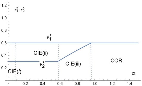
Figure 2.
Comparative statics for prices: the case of low consumers’ income.
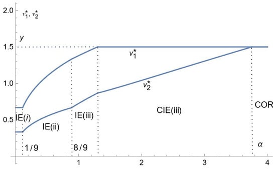
Figure 3.
Comparative statics for prices: the case of intermediate consumers’ income.
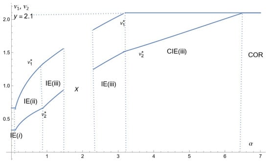
Figure 4.
Comparative statics for prices: the case of high consumers’ income.
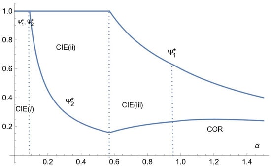
Figure 5.
Comparative statics for advertising intensities: the case of low consumers’ income.
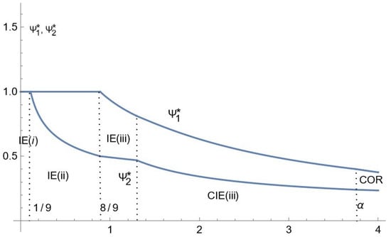
Figure 6.
Comparative statics for advertising intensities: the case of intermediate consumers’ income.
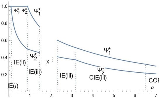
Figure 7.
Comparative statics for advertising intensities: the case of high consumers’ income.
Corollary 1
(Prices and advertising intensities). At the equilibrium (whenever it exists), the high-quality firm charges a higher price and advertises more (in a broad sense) than the low-quality one.
The proof corresponds to the representation of the relative prices and advertising intensities given in Proposition 1 in each case (low, intermediate and high consumers’ income), as a function of .
The variation of prices with is as expected. The higher , the higher the relative advertising cost, and the higher they have to set prices in order to cover their costs.
Also, as expected, the equilibrium price of the high-quality firm is always larger (in a broad sense) than the equilibrium price of the low-quality one, and the high-quality firm advertises more (in a broad sense) than the low-quality one.
Interestingly, for high enough , both prices become equal (to the consumer’s income), while Firm 1 invests more in advertising than its rival. Hence, for high enough (high advertising cost and/or low-quality differential), the price can not signal quality, whereas the advertising intensity may do so. On the contrary, for low enough (a low advertising cost and/or high-quality differential), the advertising intensities are both equal to 1, while prices are distinct, with Firm 1 charging the highest price. Hence, for low enough , the advertising intensities cannot serve as a signal of quality, whereas prices may do so.
As for advertising intensities, they are decreasing with , that is decreasing with the advertising cost butincreasing with the quality differential12, except for Firm 2 in the case of low consumer’s income under CIE (iii) and a part of COR (Figure 5). Indeed, increasing has two contradictory effects on advertising intensities. It has a direct negative effect as relative advertising costs are higher. As it thus discourages the competitor’s investment in advertising, it has an indirect positive effect: the less the rival firm invests in advertising, the more a firm is encouraged to do so. It appears that the direct negative effect is dominant except for Firm 2 in the case of the low consumer income for some range of .
Corollary 2 provides the comparative statics for the firms’ profits. Figure 8, Figure 9 and Figure 10 depict the relative profits at equilibrium, respectively, in the cases of the low, intermediate and high consumer income.
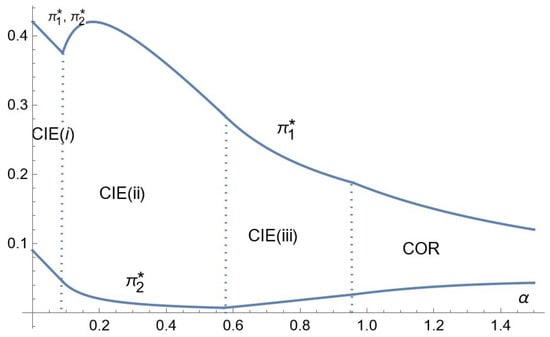
Figure 8.
Comparative statics for profits: the case of low consumer income.
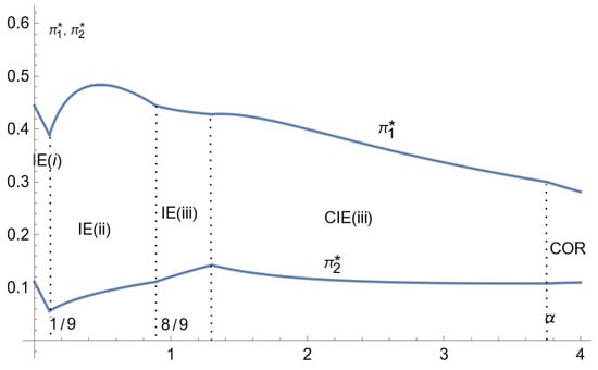
Figure 9.
Comparative statics for profits: the case of intermediate consumer income.
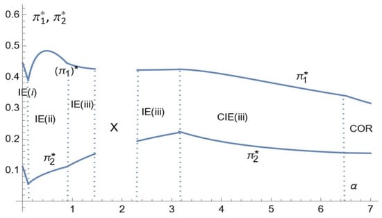
Figure 10.
Comparative statics for profits: the case of high consumer income.
Corollary 2
(Profits). The high-quality firm makes a strictly larger profit than the low-quality one. Both profits converge to zero as α goes to infinity.
To prove the result, we just represent the two firms’ profits as function of in the three cases of consumer income.
Note that even if the firms’ prices become equal beyond some critical value of , this is not profit destructive: profits are always positive. In fact, when firms charge the same price, they maintain differentiation through distinct advertising intensities.
The variation of the profit functions with the cost parameter is qualitatively the same across firms. The profit of each firm goes through three phases: at Phase 1, it is decreasing, at Phase 2, it is increasing, and at Phase 3, it is decreasing. Both profits converge to zero as goes to infinity.
An increase in the relative advertising cost parameter has a direct negative effect on the firms’ profits, which equals for Firm . This is the only one over the range of , over which they both reach all the customers; the equilibrium prices and advertising intensities do not depend on Outside of this range, there is, in addition, a positive strategic effect: an increase in the advertising cost raises the rival’s equilibrium price (Figure 2, Figure 3 and Figure 4) and generally lowers its equilibrium advertising intensity (Figure 5, Figure 6 and Figure 7). In the exceptional case where the advertising intensity of Firm 2 is increasing (over a range of in the case of low consumers’ income, Figure 5), the mild increase in has a negative strategic effect on Firm 1’s profit. As a result, Firm 1’s profit is strongly decreasing on that range Figure 5 and Figure 8).
Corollary 3 is about the profits ratio, i.e., Firm 1’s profit over Firm 2’s profit. Figure 11, Figure 12 and Figure 13 depict the profits’ ratio as a function of the relative advertising cost, respectively, in the low, intermediate and high consumers’ income.
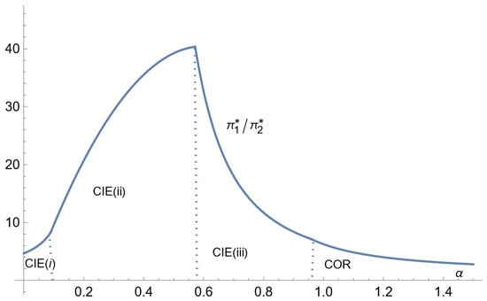
Figure 11.
Comparative statics for the profits’ ratio: the case of low consumer income.
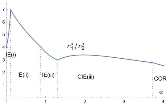
Figure 12.
Comparative statics for the profits’ ratio: the case of intermediate consumer income.
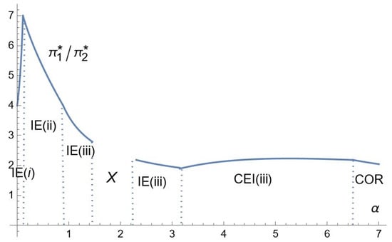
Figure 13.
Comparative statics for the profits’ ratio: the case of high consumer income.
Corollary 3
(Profits ratio). In all cases of consumers’ income, the profits’ ratio () is increasing for low enough α and decreasing above some critical level of α, converging to 1, as α goes to infinity.
The proof consists once more in representing the ratio as function of in each case, in terms of the consumer income.
It appears that the profits’ ratio in the three cases goes first (for low ) through a strongly increasing phase, during which, the higher , the more it pays to be the high-quality firm. Indeed, for low , both firms reach all consumers who are thus aware of the existence of both products, which is to the advantage of the high-quality firm (Firm 1) that thus has the possibility of charging a much higher price than its competitor. As increases, remaining in a range close to zero, the profits’ ratio equals . In the case of low consumers’ income, it occurs under CIE (i), with and ; and in the two cases of intermediate and high consumers’ income, it occurs under IE (i) for which and . In all cases, the strong increase in the profits’ ratio with is the result of a purely mathematical mechanism.
Now, as increases more, in the case of low consumers’ income, we enter zone CIE (ii), and the profits’ ratio continues to increase, and in the two other cases, we go into IE (ii); the profits’ ratio begins to decrease. We explain this contrasted effect as follows. In zone CIE (ii), while Firm 1’s price and advertising intensity remain constant, Firm 2’s advertising intensity is strongly decreasing. Firm 2’s profit is affected only by a direct negative effect, while Firm 1’s profit benefits from an indirect positive effect through the decrease in , resulting in an information advantage of the high-quality firm. In zone IE (ii), however, Firm 2 benefits from a positive indirect effect through the increase in Firm 1’s price, which outweighs the negative direct effect.
In the three cases, when goes beyond some critical value, we go into zone CIE (iii), and upon entering this zone, the profits’ ratio begins to decrease in the case of low consumers’ income, while it begins to slightly increase in the two other cases. This contrasted effect is explained as follows. In the case of low consumers’ income, the advertising intensity of Firm 2 begins to increase in zone CIE (iii), while Firm 1’s advertising intensity begins to decrease, which reduces the informational disadvantage of Firm 2, and allows it to charge a higher price ( increasing), resulting in a decreasing profits’ ratio. In the case of intermediate and high consumers’ income, both advertising intensities are decreasing, but only Firm 2’s price is increasing, while Firm 1’s price is constant when it is equal to the maximal value. Both profits bear direct negative effects of increasing . Firm 1 benefits from a positive indirect effect through the increase in Firm 2’s price and the decrease in its advertising intensity. It turns out that this is to the advantage of Firm 1, which results in an increasing profits’ ratio. But, this increase is only slight, as the effects on both firms are comparable.
As goes beyond some critical level, in all cases, the profits’ ratio decreases and converges to one. Indeed, for a high enough , both prices become equal and both advertising intensities converge to zero. Hence, as increases beyond a critical level, less and less consumers are aware of the existence of the products and thus of the advantage of the high-quality firm. It pays less and less to be the high-quality firm, as it is already constrained by the consumer’s income in terms of pricing and benefits less and less from the high-quality status because of the lack of information.
5. Conclusions
In this paper, we studied mass advertising for vertically differentiation products, whereas it has been studied only for horizontally differentiated products. This has allowed us to analyze the way the different variables (prices, advertising intensities and profits) vary with key parameters, possibly in different ways for high- and the low-quality firms. We showed, in particular, that the high-quality firm has larger prices, advertising intensities and profits than the low-quality one, but that the gap eventually shrinks as the relative advertising cost increases. We showed that the proportion of consumers who receive advertisements is increasing with the quality differential.
We qualified the result put forward by Tirole (1988) [7], according to which the equilibrium profits first decrease with the advertising cost, due to the direct effect, before they increase due to the strategic effect. We indeed found that there are three phases rather than two: profits first decrease, then increase; but, they finally decrease again with the relative advertising cost.
Besides the specific comparative statics results following from addressing the vertical differentiation case, there is a methodological contribution of this paper. We indeed showed that without an upper limit on prices, there is no pure strategy equilibrium for a relative advertising cost above some critical level13, because firms would benefit from deviating by posting very high prices and selling only to customers uninformed of the existence of their rival. Introducing, accordingly, an upper bound on prices then led us to discover the existence of two other types of equilibria, constrained interior and corner ones, which were overlooked by the existing literature.
This paper has assumed a number of simplifying hypotheses. First, it would be more natural to assume asymmetric marginal costs, with higher quality firms bearing higher marginal costs. Second, we supposed that firms use random (mass) advertising. An interesting, if unnecessary, extension will be to consider the alternative case of targeted advertising and to observe whether our results are robust. Finally, we supposed that advertising is trusted. If this hypothesis is relaxed, we will have to introduce the cost incurred by the firm in case a consumer realizes that he has been wronged; the probability that this happens is a function of the difference between the announced and the actual values.
Author Contributions
Conceptualization, R.L.-A. and D.L.; methodology, R.L.-A. and D.L.; software, R.L.-A. and D.L.; validation, R.L.-A. and D.L.; formal analysis, R.L.-A. and D.L.; investigation, R.L.-A. and D.L.; resources, R.L.-A. and D.L.; data curation, R.L.-A. and D.L.; writing—original draft preparation, R.L.-A. and D.L.; writing—review and editing, R.L.-A. and D.L.; visualization, R.L.-A. and D.L.; supervision, R.L.-A. and D.L.; project administration, R.L.-A. and D.L.; funding acquisition, R.L.-A. and D.L. All authors have read and agreed to the published version of the manuscript.
Funding
This research received no external funding.
Data Availability Statement
No new data were created or analyzed in this study. Data sharing is not applicable to this article.
Acknowledgments
We are grateful to Ibrahim Ayed for his very helpful assistance.
Conflicts of Interest
The authors declare no conflicts of interest.
Appendix A. Definition of Zones
Zone (IE)
- (i)
- (ii)
- (iii)
- Let be the equilibrium value of as a function of , and write the equilibrium profit of Firm 2 as ,
Zone (CIE)
- (i)
- .
- (ii)
- and
- (iii)
- and ,wherecorresponds to the price equilibrium of case IE (iii).
Zone (COR)
Proposition A1.
Details for Proposition 1 Zone IE (iii). At the equilibrium, advertising intensities are such that
with equilibrium relative prices of
where
Zone CIE (iii). At the equilibrium, the low-quality firm’s relative price is the real solution of the third-order polynomial, etc.
That is: where and .
Appendix B. Proofs
Proof of Proposition 1.
Elimination of the trivial solution
More precisely, if , then necessarily . Indeed, with a null price, a firm has no revenues and should not invest in advertising.
However, does not correspond to an equilibrium. Indeed, for , the profit of Firm 1 is given by: , which is not maximal at .
First-Order Conditions with a positive natural market for each firm ().
Given the expressions of the profits provided in Equations (3) and (4), the profit maximization by Firms 1 and 2 under the constraints with the associated non-negative Lagrangian multipliers yields the necessary conditions:
At the equilibrium, , for .
Indeed, if one of the , then necessarily, by Equations (A2) and (A3), the second . Hence, by Equations (A4) and (A5), prices are . But, , hence , then . But, we have just proved that does not correspond to an equilibrium.
Second-Order Conditions: Any solution to Equations (A2)–(A5), such that corresponds, for each firm, to a profit maximum.
Indeed, as , Equation (A2) implies , which corresponds precisely to , which is thus equal to zero. We prove, similarly, that .
The Hessian matrix for Firm 1 is given by:
which is a definite negative.
As for Firm 2,
which is also a definite negative.
We now deal with four possible cases, depending on whether the constraints are binding or not. One of them turns out to never be possible.
Case (i): Both firms reach all customers.
Both constraints are binding, so that There is a unique solution of Equations (A2)–(A5), which is The condition is necessary and sufficient to ensure that both multipliers are indeed non-negative. Finally, as both , the solution corresponds to a maximum for each firm.
Case (ii): Firm 1 reaches all customers, Firm 2 only a fraction of them.
We must then have and Solving Equations (A2)–(A5), we obtain a unique solution, which is and Notice that is non-negative if , while iff
As both , then the solution corresponds to a maximum for each firm.
Consequently, case (ii) corresponds to an equilibrium if
Case (iii): Both firms reach only a fraction of customers (interior equilibrium).
Here, Let us first solve for advertising rates as functions of prices. We obtain:
We decompose the reasoning into three steps in order to facilitate the reading.
Step 1: We prove that there is no equilibrium, such that and/or
(a) Consider first From (A6), it follows that Now, from Equations (A4) and (A5), , so that
Now, from (A2), for , , which implies and then
(b) Consider then From (A2), we obtain and then
As shown above, however, we cannot have at the equilibrium.
Step 2: A necessary and sufficient condition for the solution.
Substituting the expressions obtained in Equations (A6) and (A7), into Equations (A2) and (A3), and accounting for the fact that at the equilibrium, one obtains the two equilibrium conditions which the equilibrium prices must satisfy:
and
We can then conclude that the equilibrium prices must satisfy
where is strictly greater than and strictly smaller than14.
Substituting this value for in (A9), we obtain that the equilibrium value of must satisfy:
Let and The equilibrium condition (A11) can be rewritten as:
Step 3: Existence and unity of the solution of Equation (A12).
Using the above change of variables and , we can write
Let us then use the equilibrium relationship to obtain
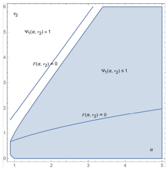
Equation (A12) has two positive real solutions which are depicted in Figure A1 in the -space using the ContourPlot function of Mathematica. In the same figure, using the RegionPlot function, we have depicted in blue the area in this space where It turns out that only the smallest solution of (A12) (corresponding to the expression of of case IE (iii) of Proposition 1) is an equilibrium. The greatest one belongs to the white area, where
Figure A1.
Representation in the -space of Equation (A12).
Denoting by , the equilibrium value from Equation (A12), we obtain that = 1 and for all
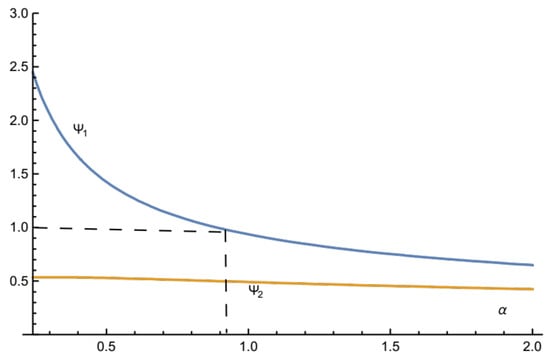
We define similarly to . We use Equation (A7), giving as a function of prices, then Equation (A10) to eliminate . We use the same change in variables to express as a function of and ; finally, we use , the value of , satisfying Equation (A12).
Plotting and on the same Figure A2, for all , we obtain that (i) , if and only if implying that the solution we just described is valid, if and only if, and (ii) .
Finally, the obtained are both positive; thus, the obtained solution corresponds to a maximum for each firm.
Case (iv): We prove that there is no equilibrium where Firm 2 reaches all consumers, while Firm 1 reaches only part of them.
Suppose this is the case; we should then have and Using the first-order conditions with regards to prices (A2), we would then obtain:
Substituting for and the above values into Equation (A4), we obtain ():
On the other hand, from Equation (A5), we obtain
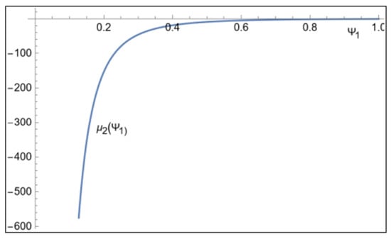
From (A14) one obtains , where the value of is the equilibrium candidate value. Substituting this value for in (A15), we should have
As pictured in Figure A3 (representing the expression given in Equation (A16)), the RHS is always negative for all values of Since the multiplier has to be positive, this does not correspond to an equilibrium.
Figure A2.
Representation of the expressions of and as functions of .
Figure A3.
Representation of the RHS of Equation (A16).
Deviations: We deal with each sub-case of case 1 to prove that no firm admits a profitable deviation.
Case (i): Here, for As long as the price candidates are less than Y, no profitable deviations exist for firms. In fact, each firm’s profit is always null outside of its natural market, as all consumers are informed of the competitor’s product, leaving no room to make a profit on uninformed ones. Hence, for the equilibrium candidate to be an equilibrium, it suffices to have .
Case (ii): Here, there is no possible profitable deviation by Firm 2, since if , for the same reason explained in case (i).
As for Firm 1, as long as , only deviations toward prices may potentially be profitable. But, if , such deviations do not exist at all.
Moreover, we know that as . Hence, the interval has a positive measure and for all , there is no deviation of Firm 1, showing that a null natural market is possible.15
Case (iii). Here, we have to consider deviations by Firm 1 and Firm 2.
Let us begin with Firm 1. We have to consider deviations in prices , resulting in a null natural market for Firm 1.
We conduct the same reasoning as in case (ii). Noting that , for all , such deviations are not possible.
Let us turn to Firm 2. The prices , such that Firm 2 has no natural market, satisfy and provide the firm the profit:
which is maximal at .
The optimal value in terms of is equal to which yields the profit:
It has to be smaller than the candidate equilibrium profit, which can be written as This is equivalent to
□
Proof of Proposition 1, Case 2 (CIE).
Given the expressions of the profits provided in Equations (3) and (4), the profit maximization by Firms 1 and 2 under the constraints and with, respectively, the associated non-negative Lagrangian multipliers and , yields the necessary conditions:
We are looking for an equilibrium such that , and each firm has a positive natural market. This necessarily implies , hence .
Now, we consider each possible case, one by one. We first write the first-order conditions allowing us to identify the candidate, then we check the second-order conditions.
(i) For from Equation (A18), one obtains This corresponds to an interior equilibrium only if
The F.O.C. with respect to (Equation (A17)), together with the condition and the expressions of and , imply
On the other hand, from condition A19 and the necessary condition , we must have
From condition A20 and the necessary condition , we must have
Notice then that whenever Thus, when , we have .
To sum up, only the conditions are necessary.
The second-order conditions.
For Firm 1, the two constraints are binding, while there are also two variables. Then, we have nothing to check for the second-order conditions.
Firm 2’s bordered Hessian, given that the constraint on is the only one active, is:
We have to consider the sign of the last principal minor, as there are two variables and one binding constraint. The last principal minor (the third) is equal to , which has the same sign as . Thus, the second-order conditions are satisfied for Firm 2.
(ii) Case and . Conducting the same reasoning as in case (i), we obtain and the necessary condition to have an interior equilibrium.
As , then and Equation (A20) implies which is smaller than 1 iff
Now, from Equation (A17) and the condition , we obtain
Using Equation (A19) and the condition , we obtain
Notice, finally, that the latter condition implies16 .
To sum up, only the conditions and are necessary.
The second-order conditions.
For Firm 1, as in case (i), there is nothing to check, since there are two variables and two binding constraints.
As for Firm 2, given that no constraint is binding, we have to consider the Hessian.
It is obviously a definite negative; thus, the second-order conditions are satisfied as well for Firm 2.
(iii) Case and . We have Using Equations (A19) and (A20) simultaneously, we express and , each as a function of the two prices, and thus obtain Equations (A6) and (A7) again. Then, we substitute these expressions into Equation (A18), which yields Equation (A9) again, i.e.:
In this equation, substitute for , for a and for , then we obtain condition (A1).
We are going to show that (1) this equation has one and only one acceptable real positive solution17 under the conditions indicated in Proposition 1 case CIE (iii); (2) otherwise (when these conditions are not satisfied), either no solution exists or the solution is not acceptable.
The derivative of with regards to is given by:
The discriminant of this second-order polynomial is given by , which is of the same sign as . The analysis depends on this sign.
(1) Suppose, first, that , and the discriminant of is always negative; thus, is always decreasing.
The limit of as goes to infinity is . Condition (A1) has one and only one real non-negative root, if and only if .
We have
(a) For , simultaneously satisfying and , , the unique real non-negative root of corresponds to an interior equilibrium only if (so that ).
Since is decreasing, in this case, and , then Equation is equivalent to , which writes as , and thus is equivalent to .
In the same way, we use the decrease in , , if and only if , which is equivalent to
We graphically prove that the two conditions and imply the condition
The interior equilibrium identified in case IE (iii) of Proposition 1 corresponds to the solution of the present system that is composed of Equations (A17)–(A20), with .
The three Equations (A18)–(A20) are satisfied here in the same way as in case IE (iii). For to correspond to the choice of Firm 1 at the equilibrium, necessarily .
Equation (A18) can we easily be rewritten (replacing with y) as
Therefore, is equivalent to .
But, we have supposed , which implies for all . Thus, . We have
This way, we have shown to be equivalent to
Finally, we consider the value of , as given by Equation (A7) and substitute Y for and for We obtain that an inequality must hold at the equilibrium.18
Graphical analysis19 shows that and g( hold when and
Second-order conditions:
Firm 1’s bordered Hessian, given that only the constraint on is active:
We have to consider the sign of the last principal minor: the determinant of the matrix, which equals , so that the SOC are satisfied for Firm 1.
Firm 2’s Hessian (since no constraint is binding) given by
is a definite negative; thus, the SOC are also satisfied for Firm 2.
(b) For satisfying but , the polynomial is decreasing with , which implies for all . This means that the profit of Firm 2 is decreasing with ; thus, the equilibrium candidate in this case is , , . The inequation is equivalent to . But, implies, on the one hand, , and on the other hand , for which the equilibrium corresponds to case (iii) of the proposition with a positive . Thus, no new case appears with a null price
(2) Suppose now that , is a second-degree polynomial that admits two roots:
and
with . is positive between the two roots and negative outside, which means that is decreasing before , increasing between and , and then begins to decrease.
We have that , which is negative when . Polynomial admits potentially three roots, depending on the sign of , and .
When they exist, these roots ( satisfy necessarily , and .
The root , whenever it exists, is never relevant because .
The root exists, if and only if, , . For this root to be acceptable, it must satisfy , and the multiplier calculated at must satisfy . Recall that
and
The representation of the set of , such that we have, simultaneously , , , and , leads to an empty set.
Finally, regarding , it exists if and only if .
Again, for this root to be acceptable, has to satisfy simultaneously , , and . And, this set is proved, graphically, to be empty.
Deviations. Finally, we have to check that, for each firm, no profitable deviation exists among the prices, such that its natural market is null20.
For Firm 1, such prices must satisfy , or equivalently . Such prices do not exist as .
As for Firm 2, the prices such that it has no natural market must satisfy , thus , or . But, this price cannot be a profitable deviation for Firm 2 as satisfies the first-order conditions over the segment of prices , and the profit is concave in over this segment; thus, it is decreasing in the neighborhood of y. □
Proof of Proposition 1, Case 3 (corner equilibrium).
We deal successively with each possible case: first, when Firm 2 has no natural market, and second, when Firm 1 has no natural market. For each case, we identify the equilibrium candidate, then check whether profitable deviations exist.
(1) If a corner equilibrium exists such that Firm 2 has no natural market, this means that , thus .
We first prove that necessarily . Indeed, Firm 1’s profit writes:
If ever then, necessarily, , which leads to profit .
Firm 2’s profit writes:
which would be maximal for . Then, Firm 1 has interest in deviating to a positive price and a sufficiently small that ensure a positive . Thus, necessarily, .
Firm 2’s profit writes:
First, note that necessarily . Indeed, otherwise the best profit in this situation would be , obtained at , whereas Firm 2 may obtain a positive profit if it deviates to a price (which is possible since ) and a sufficiently small .
Hence, is increasing with . Thus, and
Firm 1’s profit
is increasing in , and then it reaches its maximum at .
The optimal value of is given by Since , then, necessarily, , or equivalently , which is thus a necessary condition. Hence, we have which implies .
Deviations: For this equilibrium candidate to be an equilibrium, we have to check whether the firms have interest in deviating.
For Firm 1, when , its profit has only one expression, given by
The best option for Firm 1 in absolute terms is the one provided by the equilibrium candidate. This implies that Firm 1 has no interest in deviating.
As for Firm 2, if ,
If , only the second line of the above profit applies. We have to consider two types of deviations: and , when and only for .
Let us begin with deviations .
The expression of for is a continuous and concave function21 in , which necessarily reaches its maximum. When an interior solution to the first-order conditions exists, it is the maximum of the function, otherwise the maximum is reached on the borders.
The first-order conditions yield:
For a deviation to a price to be non-profitable, it is necessary and sufficient that , which is equivalent to
As , this implies . Condition (A21) is thus more constraining than , and the couple of conditions reduces to the only condition (A21).
The proof ends here when .
For and supposing condition (A21), we have also to consider deviations to prices , for which the profit writes:
which increases with and concave in . Thus, the best deviation of this nature is
Note that condition (A21) implies (or, equivalently, ), so that The resulting profit is then equal to
which is smaller than the equilibrium candidate profit , if and only if But, , meaning that condition (A21) implies This ends the proof for the corner equilibrium, such that Firm 2 has no natural market.
(2) We now deal with possible corner equilibria, such that Firm 1 has no natural market. We first identify the equilibrium candidate; then, we consider deviations. We will prove that the identified equilibrium candidate does not resist to unilateral deviations, thus it is not an equilibrium.
That Firm 1 has no natural market means that , i.e., . This necessarily implies .
Firm 1’s profit is then given by:
Then, necessarily at equilibrium. is then increasing in , thus and
As for Firm 2, with Hence, and , which is necessarily .
At this step, is a necessary condition.
Deviations: Now let us deal with the deviations.
We focus on Firm 2. Firm 2’s profit for all possible prices is given by:
The identified equilibrium candidate corresponds for Firm 2 to the best and for ; thus, there exist no profitable deviations by Firm 2 among these prices.
We now consider the deviations to prices such that . is a concave function in . The first-order condition with regards to is independent of and gives:
For deviations to such prices to be non-profitable, it is necessary and sufficient to have , which is equivalent to
But, may have two expressions.
When , then and Equation (A22) are equivalent to or equivalently .
When , then and Equation (A22) are equivalent to .
We consider now the deviations of Firm 1. Firm 1’s profit writes:
We consider first the deviations of Firm 1 to prices , such that . For such prices, which is a concave function in . The first-order condition, with regards to and independent of , yields:
For such deviations to be non-profitable, it is necessary and sufficient to have , which is equivalent to .
Considering , the profit is increasing in . When , is increasing for all prices, reaching its maximal value at . Hence, no deviation is profitable for Firm 1. □
To summarize, the equilibrium candidate is an equilibrium if and only if satisfies either condition 1 ( and ) or condition 2 ( and and ).
As depicted in Figure A4, when one condition 1 is satisfied, another condition 1 () is violated. Figure A5 shows also that no satisfies all conditions 2.
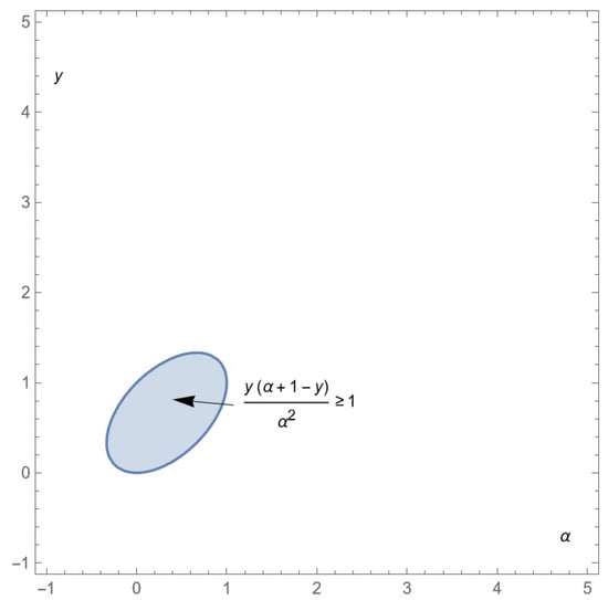
Figure A4.
Representing Conditions 1 in the -space.
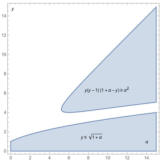
Figure A5.
Representing Conditions 2 in the -space.
Notes
| 1 | We assume that this information, notably the one on product quality, can be trusted, for instance because false advertising is banned or because quality amounts to some verifiable characteristics. |
| 2 | While here this limit comes from the fact that prices cannot exceed consumers’ income, it could alternatively be derived from the existence of a maximum utility level from consuming the good. |
| 3 | In contrast, in horizontal preferences models, consumers have different choices between variants sold at the same price. This is the case in the spatial competition models, such as the well-known Hotelling (1929) [3] model. |
| 4 | and also in terms of the “perceived consumer effectiveness” (PCE), i.e., their perceived belief in that her/his purchase will prove to have an actual effect (Nurse et al., 2012) [5]. |
| 5 | the natural market of a firm is composed of consumers who, when informed of both products, will choose the firm’s product. |
| 6 | We rule out the possibility of using misleading advertisements. We think that firms have all the less interest in deceiving consumers as, in real life, consumers increasingly may seek information on past experiences and have the option of returning products when they are not satisfied. |
| 7 | The same proviso obviously applies. |
| 8 | This is not the only possible option. We could have adopted a two-step game, where advertising intensities are chosen prior to prices, or the other way around. We may think that advertising is a decision as flexible as prices, at least in some industries, for which the static game adopted is appropriate. |
| 9 | Appendix A provides more details on the equilibrium outcome. |
| 10 | More details may be found in Appendix A. |
| 11 | The only one identified in the literature. |
| 12 | In this sense one can say that more differentiated industries advertise more. |
| 13 | Such that the high-quality firm reaches all customers for values below the critical one |
| 14 | Implying that |
| 15 | This implies , because |
| 16 | This can be observed by using Mathematica’s RegionPlot function. |
| 17 | It is too long to be reproduced here. |
| 18 | is too long to be reproduced here. |
| 19 | Using the RegionPlot function of Mathematica. |
| 20 | No profitable deviation exists among the prices, ensuring for the firm the whole market as a natural market. |
| 21 | The Hessian matrix is a definite negative. |
References
- Gabszewicz, J.J.; Thisse, J.F. Entry (and exit) in a differentiated industry. J. Econ. Theory 1980, 22, 327–338. [Google Scholar] [CrossRef]
- Shaked, A.; Sutton, J. Relaxing Price Competition Through Product Differentiation. Rev. Econ. Stud. 1982, 49, 3–13. [Google Scholar] [CrossRef]
- Hotelling, H. Stability in competition. Econ. J. 1929, 39, 47–51. [Google Scholar] [CrossRef]
- Reeve, J. Understanding Motivation and Emotion, 7th ed.; Wiley: Hoboken, NJ, USA, 2018. [Google Scholar]
- Nurse, G.; Onozaka, Y.; McFadden, D.T. Understanding the Connections between Consumer Motivations and Buying Behavior: The Case of the Local Food System Movement. J. Food Prod. Mark. 2012, 18, 385–396. [Google Scholar] [CrossRef]
- Grossman, G.M.; Shapiro, C. Informative advertising with differentiated products. Rev. Econ. Stud. 1984, 51, 63–81. [Google Scholar] [CrossRef]
- Tirole, J. The Theory of Industrial Organization; MIT Press: Cambridge, UK, 1988; pp. 292–294. [Google Scholar]
- Butters, G. Equilibrium distributions of sales and advertising prices. Rev. Econ. Stud. 1997, 44, 465–491. [Google Scholar] [CrossRef]
- Roy, S. Strategic segmentation of a market. Int. Ind. Organ. 2000, 18, 1279–1290. [Google Scholar] [CrossRef]
- Celik, L. Strategic Informative Advertising in a Horizontally Differentiated Duopoly; Mimeo, CERGE-EI 2008, Working Paper Series; Center for Economic Research and Graduate Education, Academy of Sciences of the Czech Republic, Economics Institute: Staré Město, Czech Republic, 2007; ISSN 1211–3298. [Google Scholar]
- Ben Elhadj-Ben Brahim, N.; Lahmandi-Ayed, R.; Laussel, D. Is targeted advertising always beneficial? Int. J. Ind. Organ. 2011, 29, 678–689. [Google Scholar] [CrossRef]
- Esteban, L.; Hernández, J.M. Endogenous direct advertising and price competition. J. Econ. 2014, 112, 225–251. [Google Scholar] [CrossRef]
- Simbanegavi, W. Informative Advertising: Competition or Cooperation? J. Ind. Econ. 2009, 57, 147–166. [Google Scholar] [CrossRef]
- Esteves, R.B.; Resende, J. Competitive targeted advertising with price discrimination. Mark. Sci. 2016, 35, 576–587. [Google Scholar] [CrossRef]
- Esteves, R.B.; Resende, J. Personalized pricing and advertising: Who are the winners? Int. J. Ind. 2019, 63, 239–282. [Google Scholar] [CrossRef]
- Iyer, G.; Soberman, D.; Villas-Boas, J.M. The targeting of advertising. Mark. Sci. 2005, 24, 461–476. [Google Scholar] [CrossRef]
- Esteban, L.; Hernández, J.M. Advertising media planning, optimal pricing, and welfare. J. Econ. Manag. 2016, 25, 880–910. [Google Scholar] [CrossRef]
- Zhang, J.; He, X. Targeted advertising by asymmetric firms. Omega 2019, 89, 136–150. [Google Scholar] [CrossRef]
- Zhang, J.; Cao, Q.; Yue, X. Target or not? Endogenous advertising strategy under competition. IEEE Trans. Syst. Man Cybern. Syst. 2018, 50, 4472–4481. [Google Scholar] [CrossRef]
- Galeotti, A.; Moraga-González, J.L. Strategic Targeted Advertising; Tinbergen Institute Discussion Paper. TI 2003-035/1; Tinbergen Institute: Amsterdam, The Netherlands, 2003. [Google Scholar]
- Colombo, L.; Lambertini, L. Dynamic advertising under vertical product differentiation. J. Optim. Theory Appl. 2003, 119, 261–280. [Google Scholar] [CrossRef]
- Tremblay, V.J.; Martins-Filho, C. A model of vertical differentiation, brand loyalty, and persuasive advertising. In Advertising and Differentiated Products; Emerald Group Publishing Limited: Boston, MA, USA, 2001. [Google Scholar]
- Tremblay, V.J.; Polasky, S. Advertising with subjective horizontal and vertical product differentiation. Rev. Ind. Organ. 2002, 20, 253–265. [Google Scholar] [CrossRef]
- Elliott, C. Vertical product differentiation and advertising. Int. J. Econ. Bus. 2004, 11, 37–53. [Google Scholar] [CrossRef]
- Esteban, L.; Hernandez, J.M. Strategic targeted advertising and market fragmentation. Econ. Bull. 2007, 12, 1–12. [Google Scholar]
- Esteban, L.; Hernández, J.M. Mass versus Direct Advertising and Product Quality. J. Econ. Theory Econom. 2018, 29, 1–22. [Google Scholar]
- Shen, Q.; Miguel Villas-Boas, J. Behavior-based advertising. Manag. Sci. 2018, 64, 2047–2064. [Google Scholar] [CrossRef]
- Johnson, J.P. Targeted advertising and advertising avoidance. Rand J. Econ. 2013, 44, 128–144. [Google Scholar] [CrossRef]
Disclaimer/Publisher’s Note: The statements, opinions and data contained in all publications are solely those of the individual author(s) and contributor(s) and not of MDPI and/or the editor(s). MDPI and/or the editor(s) disclaim responsibility for any injury to people or property resulting from any ideas, methods, instructions or products referred to in the content. |
© 2024 by the authors. Licensee MDPI, Basel, Switzerland. This article is an open access article distributed under the terms and conditions of the Creative Commons Attribution (CC BY) license (https://creativecommons.org/licenses/by/4.0/).