Article

A Qualitative Game of Interest Rate Adjustments with a Nuisance Agent

by
Jacek B. Krawczyk
1,*,† and
Vladimir P. Petkov
2,†
1
School of Mathematics and Statistics, The University of Sydney, Sydney, NSW 2006, Australia
2
School of Economics and Finance, Victoria University of Wellington, Wellington 6011, New Zealand
*
Author to whom correspondence should be addressed.
These authors contributed equally to this work.
Games 2022, 13(5), 58; https://doi.org/10.3390/g13050058
Submission received: 17 June 2022 / Revised: 17 August 2022 / Accepted: 19 August 2022 / Published: 29 August 2022
(This article belongs to the Section Applied Game Theory)

Abstract

:
A qualitative game describes a situation in which antagonistic players strive to keep the evolutions of their state variables in predetermined constraint sets. We argue that a qualitative game model is a suitable mathematical representation of the struggle between a domestic central bank of a small open economy and a foreign central bank of a large economy to maintain their respective state variables within an acceptable band regardless of the other player’s choices. The actions of the foreign central bank affect the domestic exchange rate and, hence, domestic inflation, output gap and interest rate. However, these actions do not necessarily aim to destabilise the small open economy, nor do they take into account the state of the latter. The domestic bank’s problem, therefore, is similar to that of a game against nature. We refer to this type of qualitative game as a nuisance-agent game (or NA-game). We use viability theory to derive satisficing rules (in the sense of Simon) of nominal interest-rate adjustments for the domestic central bank of a small open economy in a qualitative NA-game against the foreign central bank.
MSC:
37N40; 91B54
JEL Classification:
C61; D9

1. Introduction

The aim of this paper is to build and explore a qualitative monetary policy game between central banks, and draw conclusions about the interest rate adjustment strategy of the central bank of a small open economy1.
A qualitative game is a mathematical model of a problem in which antagonistic players do not maximise their respective utility functions (see [2]), but, instead, each of them strives to keep his2 own state variables in a constraint set, using his available instruments. Our model features two players: a domestic (or “local”) central bank and a foreign central bank. The actions of the latter impact former through the exchange rate between these countries’ currencies. We assume that the domestic economy is small, while the foreign economy is large. The central bank of the domestic economy will be trying to keep the country’s inflation (and, possibly, other key economic indicators such as output gap) in a predetermined set, allowing for the other country’s monetary policy. Problems of that class were introduced in the set-valued analysis literature, of which [2] is a leading example, in an abstract and general context. In that literature, the foreign player would actively seek to push the local competitor outside his constraint set. In our game, the foreign central bank does not intend to destabilise the local economy or to keep it in a specific set. The foreign bank could therefore be called a nuisance agent (rather than evil, as the players in [2] or adversary agents in other strands of economic literature tend to be called). Therefore, our qualitative game is effectively a game-against-nature (See e.g., [3] or [4].), and for brevity in this paper will be referred to as a “nuisance agent game” (or “NA-game”).
We note that the monetary policy problem of a small open economy, when a foreign country’s monetary strategy has to be allowed for, can be framed as a robust control problem as in, e.g., [5,6,7]. It could also be formulated as a minimax problem à la [8]. The main difference between those approaches and ours is that the robust and minimax control problems yield a sole robust strategy, while our qualitative game approach delivers a whole array of satisfying policies that the central bank’s governor can pick from according to his priorities (compare [9,10]). Moreover, our qualitative game framework does not require the specification of a utility function, so the underlying game model involves fewer parameters than optimisation-based models. Consequently, it is less vulnerable to the Lucas critique.
The central bank in a country such as New Zealand is in charge of maintaining price stability and supporting sustainable employment (with the latter being closely related to the output gap). This suggests that a sole optimal solution is not a priority for the bank: its mission can be accomplished with multiple combinations of inflation and output gap values, and adjustment paths leading to one of these. Indeed, even if some central banks compute an optimal interest rate policy that minimises a loss function, they do not always follow this policy in reality. Instead, they may implement it in a modified form (e.g., because of some exogenous considerations), they might utilise a Taylor-like rule, or apply an ad hoc strategy. In any case, they take into consideration the future states of the economy that can be reached from the present state using acceptable interest-rate adjustments. This sort of reasoning can be modelled rigorously with the help of viability theory, and in particular as a qualitative game.
To better justify the viability-theory framework within which we study the monetary policy problem, we invoke the idea of Herbert A. Simon (1978 Economics Nobel Prize laureate) that many economic agents use satisficing (his neologism), rather than optimising, strategies. In our view, the central bank’s behaviour is consistent with this class of strategies. Specifically, the bank seeks a satisfying policy that will keep inflation in check and will preclude major social problems such as high unemployment or an exchange rate crisis. We believe that an economic theory that follows Simon’s prescription provides a more accurate description of agents’ behaviour in the real world. We also think that viability theory (in the spirit of [11,12]) rigorously captures the essence of satisficing. Its usefulness in macroeconomics has been demonstrated by [13], who solve the monetary policy problem of a central bank in a stylised closed economy, and by [10] who study its open economy counterpart. The present paper extends their analysis by incorporating a link between the exchange rate and the foreign central bank’s actions.
In 2022, many economies experienced a significant spike in inflation. A recent article in [14]) alleges that the Federal Reserve “has made a historic mistake on inflation”. We see merit in this claim and contend that many other central banks also have erred in their approach to the inflation problem. We propose that the qualitative NA-game model examined in this paper may be of assistance to central banks. In particular, it may help the central bank of a small open economy formulate a policy of timely interest rate adjustments that could allow it to control inflation. In our model, such a policy is a function of the distance between the current state of the economy and the viability kernel boundary (see [15]). In the present paper, we show, among other things, how to compute the viability kernel for a small open economy.
In the next section, we provide a brief introduction to viability theory. In Section 3, we construct a monetary policy game model of a small open economy that interacts with a “nuisance” agent (or a NA-game). In Section 5 and Section 6 we use a viability analysis to solve the qualitative NA-game at hand. The paper ends with concluding remarks.

2. What Are Viability Problems and Their Solutions?

2.1. The Meaning of Viability

Viability theory is an area of mathematics concerned with viable evolutions of dynamic systems that are subjected to constraints on states. For controlled dynamic systems, this definition extends to allow for constraints on controls.
A system’s evolution is considered viable if the system’s trajectory remains, for the entire time of the evolution, within a prescribed region of the state space, referred to later as the constraint set K. A viability domain D is a subset of this set such that, given a constrained control set U, evolutions that originate at any point of the domain can be controlled to remain within K. The basic problem that viability theory attempts to solve is to determine whether a non-empty domain exists, and if so, what its boundaries are. The viability kernel V F K is the largest viability domain, where F denotes the system’s dynamics i.e., the collection of equations and inclusions of motion of the dynamic system (see (3) below).
In other words, the viability kernel is the set of all initial conditions for which a control strategy exists such that each trajectory originating in the kernel remains in the constraint set while the controls stay in U.
Environmental policy design has so far been the most popular social sciences problem solved by viability-theory methods. Here we cite [9,16,17,18,19] among others. Viability theory applications in other economic areas include: finance—[20]; managerial economics—[21]; macroeconomics—[10,13,15,22,23,24,25,26,27,28]; and microeconomics—[29]. Notwithstanding the economic applications, of which we address one in this paper, the viability theory has been applied to other problems where the uniqueness or optimality of the control strategy is not of major concern.
The viability kernel is the solution to a viability problem. Establishing it, will enable us to analyse the system’s transition trajectory at some distance from a steady-state rather than toward the steady-state, as in the classical analysis. We believe that an evolutionary analysis enabled by viability theory gives us a better insight into the system’s economics than just an equilibrium analysis.
We reproduce Figure 1 from [30] for an illustration of the viability idea.
The state constraint set K is represented by the yellow (or light shaded) round contour contained in state-space X. The solid and dashed lines symbolise system evolutions, which converge to where the arrows end.
The brown (darker) shaded contour is the viability kernel V F K . The trajectories that start in the kernel remain in K, hence are viable. The viability property is not satisfied by the other trajectories which start outside the kernel and leave K in finite time.
A rigorous introduction to viability theory can be found in [11,31,32], Veliov [33]. For a basic introduction to applications of viability theory see [30]. Here, we will present only these notions of viability theory that are essential to the understanding of our treatment of the monetary policy model with a “nuisance” agent (see later in Section 3 and Section 5).

2.2. Mathematical Formulation

Consider a dynamic system on the horizon Θ , where Θ can be infinite or finite, with n state variables x ( t ) R n and m control variables u ( t ) R m . Let F be a set-valued map from system’s states to the set of possible state velocities x ˙ R n .
In control theory, the multivalued map F has the form F ( x ) = f ( x , U ) = { f ( x , u ) ; u U } , where f : R n × U R n is a continuous vector-function composed of the right-hand sides of the system’s equations of motion and U is a compact set in R m . The control choices u ( t ) can depend on the state x ( t ) at which the system occurs to be. If so, the set of controls is U ( x ( t ) ) and the dynamic system is described as
x ˙ ( t ) = f ( x ( t ) , u ( t ) )
u ( t ) U ( x ( t ) ) .
In viability theory, the differential inclusion,
x ˙ ( t ) F ( x ( t ) ) ,
is the basic tool of equivalent description of the dynamic system (1) and (2). It states that at x ( t ) the change in the system’s state—its velocity—will be a member of F ( x ( t ) ) , where F is, as above, the set-valued map from system states to sets of possible velocities.3
Many economic systems can be formulated in such terms. For example, in the fishery-management problem considered in the subject literature (commented on above), the immediate future fish biomass will be in a cone determined by the apex at the present state and rays corresponding to different fishing strategies. In a monetary policy problem, the next point in time inflation will be in a cone with the apex where the current inflation is and whose rays depend on the change in the nominal interest rate.
Let K represent the closed set of constraints that state x ( t ) must satisfy for all t. The set K is an abstraction of all relevant state constraints for the problem. Given a set-valued map F : K X , we say that x 0 K X is viable in K under F if at least one solution to the system:
t Θ x ( t ) K , x ˙ ( t ) F ( x ( t ) ) ,
originates at x ( 0 ) = x 0 and remains in K forever, i.e., Θ [ 0 , ) .4 A philosophical interpretation can be attributed to the above model: an evolution that starts at a viable point follows a path that satisfies fate F and desire (or craving) K.
Formulation (4) allows us to talk about the viability of an individual system’s state. Comments on viable areas are provided in Appendix A.
We can say that a viable strategy is a realisation of a satisficing policy postulated in [34]—so long as viability is not threatened, any control is “good enough”. It is our belief that such characterisations of economic states provide a good description of the decision-making behaviour of managers in the “real world”. In particular, inflation-targeting central banks will often avoid changing interest rates for as long as they can.
It might be argued the current inflation in many countries is due to the central banks’ unawareness of their respective viability kernel boundaries. Would policy-makers have been aware that the economic states are approaching a viability kernel boundary whose crossing makes it impossible to contain inflation through a smooth interest rate adjustment, they would have acted earlier. It seems plausible that central banks would want to know the kernel’s boundary (to avoid a crisis management control à la see [35,36]), at which the pace of interest rate adjustment would have to be accelerated. We contend that central bank management strategies based on viability analysis will be closer to how managers actually want to deal with their problems.
We also want to stress that there is a crucial difference between the optimisation approach and the viability approach to modelling dynamic systems. A viability-theory problem formulation does not include a utility, or loss, function, and explicitly defines the set of acceptable states K. A solution to the viability problem consists of a multiplicity of satisficing controls. In the optimisation approach, the constraints that represent K are usually implicit in the loss function and the resulting solution is typically a unique control strategy. A concise discussion on this rather orthogonal relationship between viability and optimality can be found in [30]. In [37], also in [13], optimal and viable solutions to a pedagogical 2D problem are juxtaposed.

2.3. A Qualitative Game

As explained in the Introduction, a qualitative game is a mathematical problem in which players do not maximise their respective utility functions, but, instead, each of them strives to keep his own state variables in a constraint set, using his instruments.
The authors of [2] trace down their work on qualitative differential games to the seminal book by [38]. They propose a model for a “target problem”, in which one of two players with coupled dynamics aims at reaching an open set O and, at the same time, avoid a closed set E . The other player seeks to avoid O until he reaches E . This game is an abstraction of a pursuit-and-evasion problem typically played on a finite horizon. A solution to such a game consists of the characterisation of the set of initial positions from which a player may win, whatever his adversary plays.
In our model, there are also two players with coupled dynamics. The first player is the domestic bank of a small open economy, whose objective is to keep the domestic economy in the closed set K (i.e., avoid being in K’s complement for all t Θ ). The other player is the bank of a large foreign economy, which pursues its own target that is unrelated to K. The dynamics are coupled through the actions of the foreign bank, which affect the domestic economy’s position. Hence, in seeking to remain in K, the domestic player must react to the foreign player’s actions.
The foreign player’s impact is filtered through the given system’s dynamics and, in our model, the domestic player will need to hedge against only one of the foreign player’s state variables. This makes our qualitative game less antagonistic than a pursuit-and-evasion problem. So, this is a qualitative NA-game (“nuisance-agent game”), as opposed to the pursuit-and-evasion problem, which is a genuine qualitative game. A solution to our game will consist of the characterisation of the viability kernel i.e., the set of the domestic player’s initial conditions, from which he may keep his states in K.
We will use a specialised piece of software VIKAASA to obtain a numerical characterisation of the viability kernel. A brief description of the software is provided in Appendix C.

3. A Macroeconomic Model

3.1. A Viability Theory Problem

In reality, central banks are often tasked to maintain a few key macroeconomic variables within predetermined bounds. Some of these bounds may result from a welfare maximisation problem solved by a social planner. Others may be exogenously imposed and politically or socially motivated. The bank can achieve these targets using an optimising solution that minimises a loss function. Typically, the central bank’s loss function will include penalties for violating allowable bands on inflation and output gap, as well as a punishment term for excessive interest rate adjustments. In a standard linear-quadratic framework, the solution that minimises the loss function is unique for a given selection of parameters. Hence, this approach does not allow for a multiplicity of strategies.
Our paper takes an alternative approach. We apply viability theory methodology to a central bank that wants to maintain economic variables of concern in a constrained set. The bank’s problem is similar to the viability theory problem (4), illustrated in Figure 1. We will characterise the set of economic states V F ( K ) that enables the central bank to keep the economy within the prescribed set K, given the set of available instruments U. The set V F ( K ) is the viability kernel.
V F ( K ) x ( 0 ) : s . t . x ( t ) starting from x ( 0 ) , satisfying ( 1 ) and ( 2 ) and constraints K t Θ .
In the next section we will examine a stylised monetary policy model (inspired by [39]; also, by [40,41]). We will then show that the solutions obtained through viability theory do not suffer from the common drawbacks of their optimisation-based counterparts.

3.2. The Central Bank’s Problem

Suppose that a central bank in charge of a small open economy such as New Zealand’s is using the nominal interest rate i ( t ) as an instrument to control inflation π ( t ) and output gap y ( t ) , and the real exchange rate q ( t ) .
Following [39], we adopt the notation as below.
I.
Output gap y ( t ) is the log deviation of actual output from “natural” output. Since this is a log deviation, it is interpreted as a fraction of natural output.
II.
Inflation is defined as the CPI inflation rate. The symbol π ( t ) denotes the deviation of CPI inflation from a reference value of inflation.
III.
Interest rate is the short-term nominal interest rate that is used by the central bank as the policy instrument. We denote the deviation of the nominal interest rate from its reference value by i ( t ) .
Both rates are expressed as fractions rather than percentages. We also follow the convention in this literature by considering annualised rates. The reference values can be steady-state values (if available) or some typical long-term averages. In this paper, we assume that the reference values of inflation and nominal interest rate are 0.02 and 0.04, respectively. Hence, the level inflation and interest rates will be π ( t ) + 0.02 and i ( t ) + 0.04 , respectively. We will use I to denote the level interest rate.
IV.
Exchange rate q ( t ) is the log ratio of
nominal exchange rate × foreign price index domestic price index .
It can be viewed as an aggregate measure of the strength of a country’s currency. If the local currency weakens, then q ( t ) increases. That is, a larger value of q ( t ) implies real depreciation: the domestic goods become relatively cheaper when q ( t ) is large. Conversely, if q ( t )  decreases, the local currency strengthens, hence the domestic goods become relatively more expensive.
Furthermore, we assume that interest rate adjustments u ( t ) are selected from a closed set U. Specifically, U is an interval [ u ̲ , u ¯ ] , where u ̲ , u ¯ R + . That is, u ̲ and u ¯ are the fastest downward and upwards interest rate adjustments, respectively. The values of u ̲ , u ¯ will depend on the bank’s view on how smooth the interest rate adjustments should be.
In the parlance of optimal control and dynamic games, the vector [ y ( t ) , π ( t ) , i ( t ) , q ( t ) ] , t Θ is the state vector for the domestic central bank. The vector’s domain is R 4 K . The control variable in this model is u ( t ) U R . The noise (disturbance) input into this model is the real interest rate of the large (foreign) economy, which is controlled by the foreign central bank. This input will be introduced in (11).
The authors of [10] examined a continuous-time state-space representation of an open economy with the following system’s dynamics:
d y d t = a y d 2 ( i π ) + d 3 q
d π d t = 2 p y
d q d t = ( i π ) ρ u
d i d t = u U ,
where all variables are in expectation. We note that this system is a differential inclusion because of (9). The parameters a , d 2 , d 3 , p , ρ are nonnegative.5 The time-dependent variables y , π , q , i , u are as defined above (to simplify the notation, we have dropped the time index t). We claim that the above model is easier to comprehend, and captures the underlying economic dynamics more succinctly than its discrete-time analogues i.e., [39,40,41]. We refer the readers to [10] for the algebra of the transition from discrete-time to continuous-time dynamics.
Equations (6)–(9) define the expected output gap (see (6)) as a (zero) mean-reverting process that is driven by the real interest rate and the exchange rate. The exchange rate determines the competitiveness of domestic goods in the world market and, as a result, affects the change in the output gap. If the domestic currency appreciates (i.e., q ( t ) diminishes), foreign goods become cheaper relative to domestic goods and the output gap shrinks. A positive deviation in the real interest rate depresses output by incentivising agents to save more and consume less, thus causing the output gap to shrink. Conversely, a negative deviation in the real interest rates stimulates output, so the output gap grows.
The expected speed of inflation (see (7)) is proportional to the expected output gap. The reason is that, in the discrete-time model of [39], inflation depends on the current as well as on the delayed output gap. In our continuous-time setting, these effects add up to the coefficient 2 p . Furthermore, in contrast to the discrete-time model of [39], the continuous-time (short-term) expected change in inflation does not depend on the exchange rate. The reason is that in [39] inflation is a function of the exchange rate difference, which tends to zero for short intervals. Therefore, q ( t ) disappears from differential Equation (7).
Equation (8) captures the process of currency adjustment to changes in the domestic real interest rate when the foreign real interest rate level remains unchanged. As explained earlier, q is the log transformation of the real exchange rate. Therefore, the derivative d q / d t is the rate of change of the real exchange rate. If the right-hand side of this equation contained only the bracketed term (i.e., the real interest rate), this would be a straightforward continuous-time version of the real interest parity condition (see [42]). Indeed, if we denote the log transformation of the nominal exchange rate by s, then by definition
d q d t = d s d t + foreign inflation domestic inflation .
After combining this relationship with the classical interest parity condition in continuous time, see ibid., we obtain the real interest parity as formulated in (10), apart from the last term whose inclusion is explained below.
If the domestic real interest rate goes up, then local bonds will earn more in domestic currency. Foreign demand for these bonds will increase, which causes the currency to appreciate. In our model, this effect is captured by the second term of the right-hand side of (8). Indeed, for u > 0 , d q / d t diminishes, so the currency appreciates (or depreciates more slowly). However, bond returns in all countries will be equalised in the long run due to arbitrage. If there is little effect on π , a higher i would imply a higher real interest rate, so possibly i π > 0 and q will grow. This means that the currency will depreciate over time, so the domestic bond yields for a foreign investor will eventually decrease to compensate for the interest rate differential.
At this stage, we need to remark that the real interest rate i π in (8) could be preceded by a coefficient that determines the speed with which the exchange rate moves up or down, given the changes on the right hand side of (8). In the above formulation, this coefficient is set to 1. Since i and π are annualised, this corresponds to q depreciating by 1 per cent annually, provided that the real interest rate is 1 per cent and there are no central bank interventions. However, as we will see in Section 4, the parameters a , d 2 , d 3 , p , ρ (borrowed from [39]) define d y / d t and d π / d t as quarterly velocities. For consistency, we define u as an admissible interest-rate adjustment per quarter, and divide the domestic and the foreign real interest rates in (10) by 4. We will revisit this issue in Section 4, where we calibrate (6)–(9).
If the expected deviation of the foreign real interest rate is zero, then it can be ignored, as in Equation (8). However, since we are explicitly interested in the interaction between foreign and domestic monetary policies, our model must account for changes in the foreign real interest rate. To allow for such changes, we modify Equation (8) as follows:
d q d t = 1 4 i ( t ) π ( t ) 1 4 i * ( t ) π * ( t ) ρ u ( t ) ,
where the foreign economy’s variables are denoted with an asterisk * .
The movements in the foreign real interest rate are a “nuisance” for the domestic bank, as they are transmitted to inflation in (7) via Equations (10) and (6).6 These movements complicate the domestic bank’s monetary policy problem, as compared to a model in which the foreign country’s real interest rate remains unchanged. From the domestic bank’s point of view, varying foreign real interest rates is a shock that needs to be hedged or attenuated.
If we assume that the foreign central bank also wants to keep its economy inside a viability kernel, then the domestic bank can expect a limited variation of the foreign real interest rate:
v ( t ) i * ( t ) π * ( t ) V ,
where V is a closed interval [ v ̲ , v ¯ ] , with v ̲ , v ¯ denoting the lowest and highest foreign real interest rates, respectively, expressed as deviations from a reference level. The allowance for the foreign real interest rate shocks transforms Equation (10) into the following differential inclusion:
d q d t 1 4 i ( t ) π ( t ) 1 4 [ v ̲ , v ¯ ] ρ u ( t ) .
The system’s dynamics (i.e., the mapping F) of the domestic bank’s monetary policy problem will then be given by:
d y d t = a y d 2 ( i π ) + d 3 q
d π d t = 2 p y
d q d t 1 4 ( i π ) 1 4 [ v ̲ , v ¯ ] ρ u
d i d t [ u ̲ , u ¯ ] .
Assume that the domestic central bank must keep inflation in a predetermined region [ π ̲ , π ¯ ] . Moreover, the bank wants to maintain some boundaries on the output gap, [ y ̲ , y ¯ ] , the interest rate [ i ̲ , i ¯ ] and exchange rate [ q ̲ , q ¯ ] , all expressed as deviations. Limiting the interest rate adjustment velocity u = d i / d t to the interval U would yield a smooth time profile of i ( t ) . Additionally, setting a (tight) band will help the private sector form expectations about the economy’s future.
As explained earlier, the motivation for the bounds on the state variables can be social (e.g., a large negative output gap and high-interest rates are associated with high unemployment), or political (e.g., exporters will not vote for a government under which the domestic currency has appreciated a lot).
Since the bank communicates its policies using the levels of inflation and interest rate, we define the constraint set K (see (4)) in the central bank’s problem as follows:
K = [ y ̲ , y ¯ ] × [ π ̲ + 0.02 , π ¯ + 0.02 ] × [ i ̲ + 0.04 , i ¯ + 0.04 ] × [ q ̲ , q ¯ ] R 4 ,
where 0.02 and 0.04 are the respective reference levels of inflation and interest rate.

3.3. How Can the Viability Kernel Be Used by the Domestic Central Bank?

Here we elaborate on the information structure within which the domestic bank operates, and explain how the computed viability kernel can help this bank conduct its policy making.
Any state inside the viability kernel V F K can be controlled with u ( t ) U , t Θ , to stay inside V F K , but no state outside V F K can. The domestic central bank knows the set of states that will allow it to keep its economy in the desired set K. The kernel is computed for the calibrated system’s dynamics (i.e., for specified values of the coefficients a , d 2 , d 3 , etc.), the interest rates adjustment speed range U and the range for the foreign real interest rate V. The ranges U and V can be assumed or inferred, and are often politically motivated.
At time t, the domestic bank observes the state vector x ( t ) = [ y ( t ) , p i ( t ) , q ( t ) , i ( t ) ] . If x ( t ) is outside the viability kernel, then some crisis control could be implemented (e.g., u ( t ) can be selected a larger set U , where U U ). If x ( t ) is inside the viability kernel, then the bank implements a viable control. By definition, each state in V F K is associated with at least one viable control, and the central bank’s governor knows that control.

4. Calibrated Qualitative Monetary Policy NA-Game

The domestic bank’s viability problem is to determine the viability kernel V F K , where K is defined by (17) and F is the point-to-set mapping (13)–(16). The kernel contains all initial positions of y , π , q and i such that at least one evolution originating from any of these positions does not leave K in finite time. This evolution must involve interest-rate adjustments u from U and foreign real interest levels v from V. If at least one such evolution exists, then the kernel is non-empty. The interest rate adjustments u that generate such an evolution constitute satisficing strategies of the domestic bank.
The viability kernel V F K K R 4 will be computed in Section 5. First, however, we need to calibrate the model (13)–(17).
We adopt the following parameter values reported by [39,43], calibrated from UK data:
a = 0.2 , d 2 = 0.5 , d 3 = 0.2 , p = 0.2 .
These papers use a quarter (i.e., 3 months) as a period of observation. Substituting these parameters in (13)–(16) gives us a calibrated model (see (20)–(23)). The values of these parameters determine the speed of evolution of our small open economy. E.g., if the output gap is kept constant at 0.01 for three months, inflation would rise by 0.004 during this time. We note that in a large closed economy inflation would have risen slower (compare [13]). This may be because a large closed economy is more inertial than a small open economy.
There is no universally accepted value for ρ , the exchange rate responsiveness to domestic bank interest rate adjustments (see inclusion (15)). In this paper, we assume that ρ = 4 . We refer the readers to Appendix B, and also to [10], for a discussion on how the value of ρ was chosen.
In recent times, interest rate adjustments have been made in an environment of high inflation that is outside the acceptable set K. Such an environment requires a crisis control strategy, see [35,36]. This would amount to widening the set U and/or shortening the interval between adjustments. Hence, the current breadth of U is probably bigger than what it would typically be. Since our model aims to show how to avoid a crisis before the economy gets stressed, we will assume that nominal interest rate adjustments are made quarterly. In the past, a typical change in the interest rate was either 0.25 per cent or nil. We will assume a “generous” interval for the possible adjustments of the domestic interest rate,
d i d t = u [ 0.005 , 0.005 ] U .
Within this interval, the interest rate i can drop or increase between 0 and 0.5 percent per quarter.
The other input into the model is the foreign real interest rate, see (11). Historical data on real-interest rate level fluctuations in the US suggest that it moves between −6% and 6% per year. Assuming 2% as the reference level, the annual deviations can be between -8% and 4%. Since all velocities in (13)–(16) are quarterly, we will assume that the variability of v per quarter is
v [ 0.02 , 0.01 ] V .
Taking into account the discussion regarding the velocity of q in Section 3.2, the our calibration exercise yields the following macroeconomic model:
d y d t = 0.2 y 0.5 ( i π ) + 0.2 q
d π d t = 0.4 y
d q d t 1 4 ( i π ) 4 u [ 0.02 , 0.01 ] .
d i d t [ 0.005 , 0.005 ] .
Next, we need to specify the constraint set K. In the past, the politically desired bounds for New Zealand’s level inflation were set by legislation to [ 0.01 , 0.03 ] . There is less consensus on what the desired output gap should be. We will assume that y ( t ) [ 0.04 , 0.04 ] . This rather wide interval for the output gap reflects a lesser concern of the central bank for y ( t ) . The acceptable range of the real exchange rate is even more debatable. We will assume an interval of [ 0.1 , 0.1 ] as a tolerable range for q ( t ) . Finally, we need to set a range for the interest rate. We assume that i ( t ) [ 0 , 0.07 ] .
Allowing for the reference levels of inflation and interest rate (see item I, page 6) yields:
K ( y , π , q , i ) : 0.04 y 0.04 , 0.01 π + 0.02 0.03 , 0.1 q 0.1 , 0 i + 0.04 0.07 .
In Section 5, we compute the viability kernel for the the calibrated dynamics (20)–(23) and the constraint set (24). Note that this is a particular specification of the general viability model (4) (on page 4).

5. Viability Analysis: Parameter-Specific Solutions

5.1. A Method for the Determination of Viability Kernels

In [44] we can find a base for how to approximate V F K using the solutions to the differential inclusion (3). In broad terms, they say that if a constrained optimal control problem, with dynamics F ( · ) and the constraint set K, can be solved for x K and x ( t ) K t , then x is viable.
VIKAASA (See [45,46]; also [9].), is a computational tool that computes viability kernel approximations (actually, domains) for the class of viability problems introduced in this paper, using a user-selected algorithm (there are two algorithms to choose from). In this paper, we have selected one that solves a truncated optimal stabilisation problem, rather than a general optimal control problem, for each x h K h K where K h is a suitably discretised K.
For each x h K h , VIKAASA assesses whether a dynamic evolution originating at x h can be controlled to a (nearly) steady-state without leaving the constraint set in finite time. Those points that can be brought close enough to such a state are included in the kernel by the algorithm, whilst those that are not are excluded.7
In Appendix C, we provide a short description of the use of VIKAASA. For extended comments on several kernel computation algorithms, we refer the reader to [9,30].

5.2. Analysing Monetary Policy in Four Dimensions

In Section 3.3, we explained the merit of using viability kernel methodology to analyse domestic interest rate adjustments. The remainder of this paper aims to illustrate this merit. Our analysis will be parameter-specific. We do not claim that our results are universal. Nevertheless, we contend that our graphical examination of the multidimensional viability kernels provides a pedagogical explanation for how the domestic bank’s reactions u U to the foreign bank’s actions v V are able to keep the state variables y ( t ) , π ( t ) , q ( t ) , i ( t ) in the desired set K V F K .
Our model yields a four-dimensional viability kernel that is not amenable to direct graphical representation. To help understand our policy analysis, we now show how to interpret 3D “slices” of this 4D kernel.

5.3. How to Interpret a 3D Projection of a 4D Kernel

Imagine that the domestic central bank surmises that the change in the foreign real interest rate is zero, i.e., v = 0 . Using VIKAASA see Appendix C, we have computed the 4D viability kernel V F K K R 4 for v = 0 , given the equations of motion (20)–(23) and the constraint set (24), as per the definition (5). In Figure 2, we show several rows of the array that contains the viable points.8
To study the bank’s monetary policy problem, we will use time profiles of key variables (see Figure 3) and 3D slices of the 4D viability kernel V F K (see Figure 4). The axes of the resulting figures are scaled in the real-life units. Inflation and interest rates are expressed in level terms. Among other things, we will show that v = 0 does not imply stationarity of the domestic exchange rate.
Now we select a point from the viability kernel (i.e., a viable point) and examine how the interest rate adjustments u ( t ) U , t [ 0 , Θ ] drive the evolution of this economy. In particular, we consider
[ y 1 ( 0 ) , π ( 0 ) , q ( 0 ) , i ( 0 ) ] = [ 0 . 0057 , 0.006 , 0.0714 , 0.002 ] .
When translated to level terms, this point is:
x 1 ( 0 ) = [ y 1 ( 0 ) , π ( 0 ) + 0.02 , q ( 0 ) , i ( 0 ) + 0.04 ] = [ 0 . 0057 , 0.026 , 0.0714 , 0.042 ] .
This point corresponds to an economy in “good shape”: output gap is mildly positive, inflation (in level terms) is not far from 2 per cent, the currency is rather overvalued and the interest rate is close to its reference value. In essence, x 1 ( 0 ) might characterise a developed economy in the time before the COVID pandemic.
We also select a point from the complement of the viability kernel (which is thus non-viable). This point is:
[ y 2 ( 0 ) , π ( 0 ) , q ( 0 ) , i ( 0 ) ] = [ 0 . 016 , 0.006 , 0.0714 , 0.002 ] .
It translates to the following level terms:
x 2 ( 0 ) = [ y 1 ( 0 ) , π ( 0 ) + 0.02 , q ( 0 ) , i ( 0 ) + 0.04 ] = [ 0 . 0016 , 0.026 , 0.0714 , 0.042 ] .
The difference with the previous illustration point is in the value of the output gap (shown in bold font).
We contend that x 2 ( 0 ) might describe a developed economy near the end of the pandemic, when unemployment is very low, but the other key variables have not yet changed from their pre-pandemic levels. We believe that comparing the evolutions of two economies that differ only in their output gaps will help the reader appreciate the benefits of using viability theory for monetary policy.
Consider Figure 3. The viable evolution originating from x 1 ( 0 ) is represented by solid lines, while the non-viable evolution originating from x 2 ( 0 ) is shown with dash-dotted lines. The figure has eight subplots. The first four track the state variables. Subplots plots 5 and 6 are the same as 2 and 3, respectively, but are scaled in level terms. Subplot 7 depicts the economy’s overall velocity9. Finally, subplot 8 shows the interest rate adjustments that keep x ( t ) , t [ 0 , Θ ] in V F K K .
The bank reacts to the mildly positive output gap (see the solid lines) by lowering the interest rate (see subplot 8, as well as subplots 3 and 6). This interest-rate adjustment prevents a sharp decline in the output gap. Over time, inflation goes down and the exchange rate decreases (q grows, hence the local currency weakens). This helps the output gap recover, and it stays mildly negative. Subsequently, the economy stabilises without further intervention. This evolution is also visible in 3D in Figure 4, which is discussed below.
The “boulders” in Figure 4 (and also in the subsequent figures) are 3D slices of the V F K R 4 , whereby the 3D space is spanned on the axes {output gap, level inflation, level interest rate}. The cuboids represent the projections of the constraint set K onto 3D space. In the left panel, the boulder is the slice of V F K through q ( 0 ) = 0.0714 . We see that x 1 ( 0 ) , the starting point of the solid line, is a boundary point of the boulder (and also of the viability kernel). The trajectory starting at this point is clearly viable, as it remains in K. It confirms the observations we made when examining the time profiles in Figure 3: the interest rate drops, and inflation and the output gap stabilise. The boulder in the right panel is the slice of V F K R 4 through inflation of 0.006 (level inflation of 0.026).
The large positive output gap in x 2 ( 0 ) threatens to cause a spike in inflation (see the dash-dotted lines). Because of the delay (“inertia”) between interest rate adjustments and their effects on the output gap and inflation, no interest rate adjustment can prevent the inflation spike in our calibrated model. Inflation will exceed the allowed upper bound, so the starting point x 2 ( 0 ) is non-viable.
If the bank stays inactive and keeps the interest rate adjustments at zero for some time, then the currency remains overvalued and the output gap diminishes rather quickly. Inflation would eventually decrease, but only after it has breached the upper bound (see subplots 2 and 5).
The above evolution and the resulting breach of the inflation bound might explain the current spike in inflation experienced by many countries. As already discussed, we do not claim that the specific times and magnitudes reported in our figures can be directly translated into real-life data. However, we argue that our model correctly captures the implications of a large output gap and overvalued currency for the economy.
The developments after the period of rising inflation and diminishing output gap (see the dash-dotted lines) reflect the bank’s attempt at stabilising the economy. Lowering the interest rates at that stage is by and large ineffective, because the output gap is already very negative, causing inflation to drop below the lower bound. The currency remains overvalued, and thus continues to depress output.
Our model and the software that computes the viable points (see Appendix C) have not produced a successful interest-rate adjustment policy for fighting a larger output gap.
The conclusion we can draw from the above discussion is that a mildly positive output gap and overvalued currency, such as at x 1 ( 0 ) , should be taken seriously. In particular, the banks should consider the proximity of the output gap to the boundary of the viability kernel (see the right panel in Figure 4). In our example, the value of the output gap in x 1 ( 0 ) is close to being critical: a slightly larger output gap would make the economy non-viable.
This proximity is evident in the right panel of Figure 4. Here the viability kernel is sliced at inflation of 0.006 (level inflation of 0.026). The boulder depicts the kernel projection onto R 3 with dimensions {output gap, exchange rate, level interest rate}. We see that the evolution of the solid line starts at a boundary of the viability kernel. This line goes through a region of the negative output gap and stabilises close to the neutral output gap. On the other hand, the dash-dotted line, which shows an evolution from x 2 ( 0 ) , breaches the lower bound of the output gap.
To summarise, an evolution that begins inside the viability kernel will not leave it in finite time. If, on the other hand, it originates from outside the kernel, it will eventually leave the constraint set K (the cuboid “box” in the figure).
We believe that analysing the viability kernel slices is instructive for understanding the topology of the multidimensional process of interest rate adjustment. A caveat of using 3D slices is that, while a viable evolution never leaves the viability kernel V F K K , it does not need to remain in the “slice”. This is because each 4D line represented in 3D is parametrised in the fourth dimension. That is, each line segment corresponds to a different value of the fourth dimension.

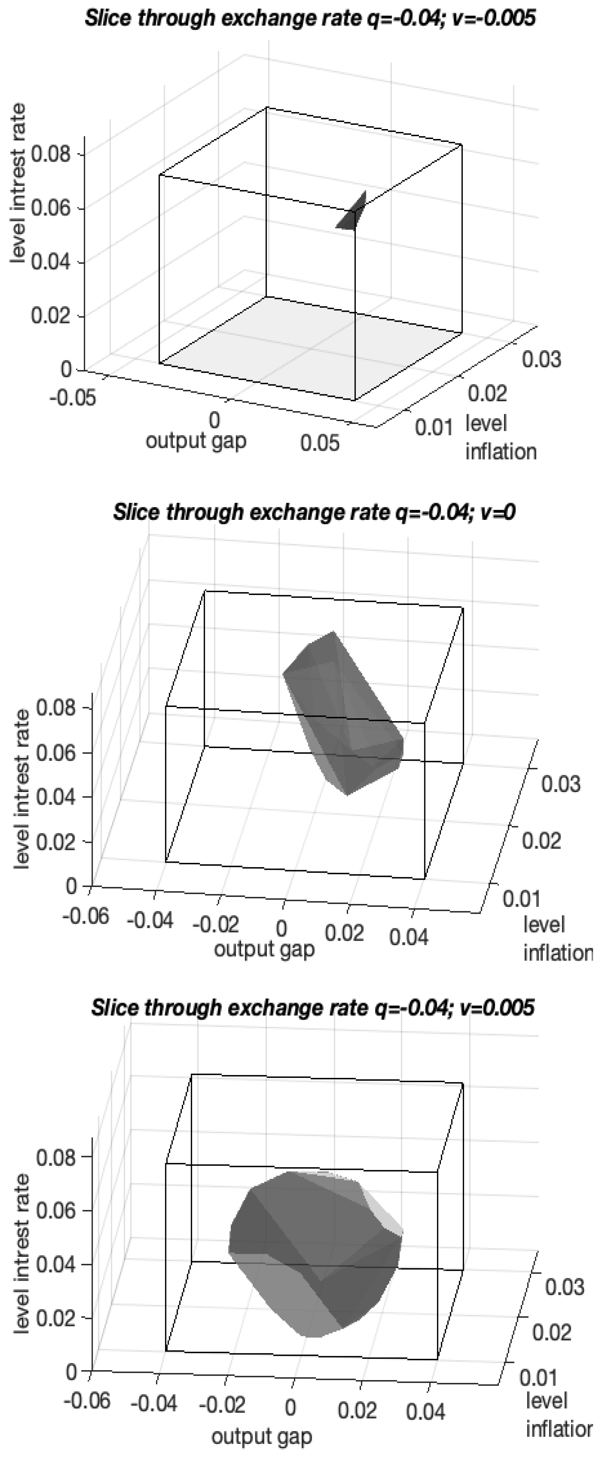
6. Impact of Foreign Real Interest Rate on the Domestic Economy

We now consider three scenarios concerning the foreign country’s real interest rate: when it is negative, neutral and positive. We model these scenarios numerically with v = 0.005 , v = 0 and v = 0.005 (i.e., −0.5%, 0% and 0.5%). Each of these values will have a different impact on the exchange rate, through which the foreign economy affects the domestic economy.

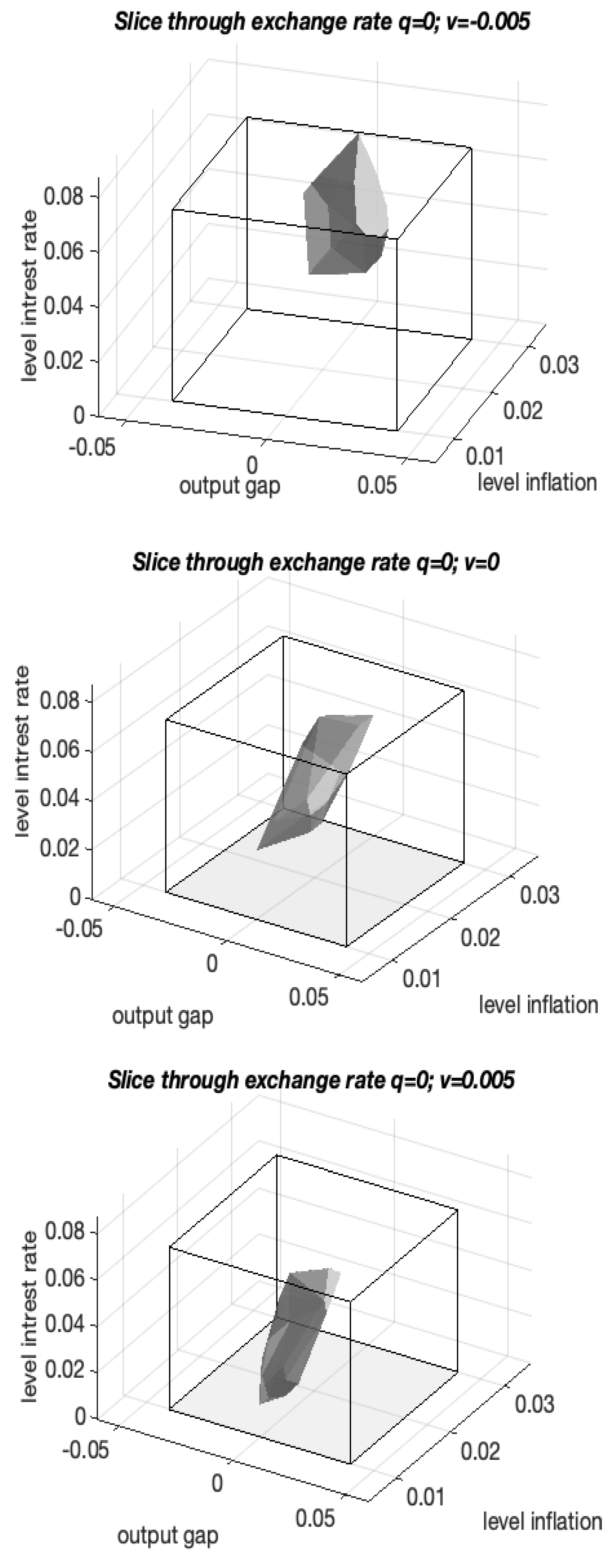
6.1. Neutral Exchange Rate

First, we examine the impact the foreign real interest rate will have on the domestic economy when the exchange rate is neutral, i.e., when q = 0 .
Figure 5 shows slices through q = 0 of the three kernels computed for foreign real interest rates of 0.5%, 0% and −0.5%. Each cuboid represents the constraint set K projected onto the space of output gap, inflation and domestic interest rates. We will refer to these cuboids as K 0 .
All three slices in Figure 5 are of commensurable volumes, i.e., they have a comparable number of viable economic states. However, these slices are located in different parts of the state space. In particular, they are (almost) vertically separated along the dimension of the domestic interest rate. The slices are also shifted horizontally relative to the centres of output gap and inflation. Therefore, the domestic economy needs to be in different areas of the state space to cope with different foreign real interest rates.
If the foreign real interest rate is negative ( v = 0.005 , top panel), then the viability kernel’s slice for q = 0 is situated in the upper part of K 0 , where the domestic interest rates are high and the output gap and inflation are slightly above their middle values. When the foreign real interest rate is neutral ( v = 0 , middle panel), the slice is in the centre of K 0 . Finally, when v is positive, the slice is in the lower part of K 0 , where the domestic interest rates are low and the output gap and inflation are slightly below their middle values.
We can provide the following intuition for why the domestic economy with a neutral exchange rate might not have a viable evolution.
Overall, a neutral exchange rate ( q = 0 ) means that the output gap and inflation are not affected by the foreign economy for as long as the exchange rate remains neutral. This may change due to domestic interest rate adjustments (see (22)).
When the foreign real interest is negative and the domestic economy is close to the upper bound on y, inflation is rather high (see the top panel) and π may go beyond its upper bound. Equation (20) suggests that high domestic interest rates are necessary to bring the output gap down, instead of just relying on a fall due to mean reversion. Increasing i requires an interest rate adjustment, u > 0 . However, this adjustment may be neutralised by v < 0 , as per (22).
In the bottom panel, we have v = 0.005 . Here, the output gap is negative and requires a stimulus to increase. This might be achieved by lowering the domestic interest rate through a negative adjustment, u < 0 . To keep the exchange rate neutral (so that q = 0 in (20)), a negative interest rate adjustment may be offset by v > 0 .
The economy in the middle panel appears not to require adjustments, so v = 0 will help keep it that way.
In summary, when v < 0 and the domestic bank chooses u > 0 or, conversely, when v > 0 and the domestic bank chooses u < 0 , domestic interest rate adjustments will have little effect on the exchange rate.
We notice that no points belong to all three slices in Figure 5. However, the top slice and the bottom slice intersect individually with the central one. We can therefore recommend to the domestic central bank that, in an environment of few domestic inflationary and output-gap pressures:
  • the bank should keep the domestic interest rate close to the upper limit when the foreign real interest rate is negative;
  • the bank should keep the domestic interest rate close to the lower limit when the foreign real interest rate is positive.
In the case when the foreign real interest rate is zero, the domestic interest rate should obviously be kept in the middle of the range.

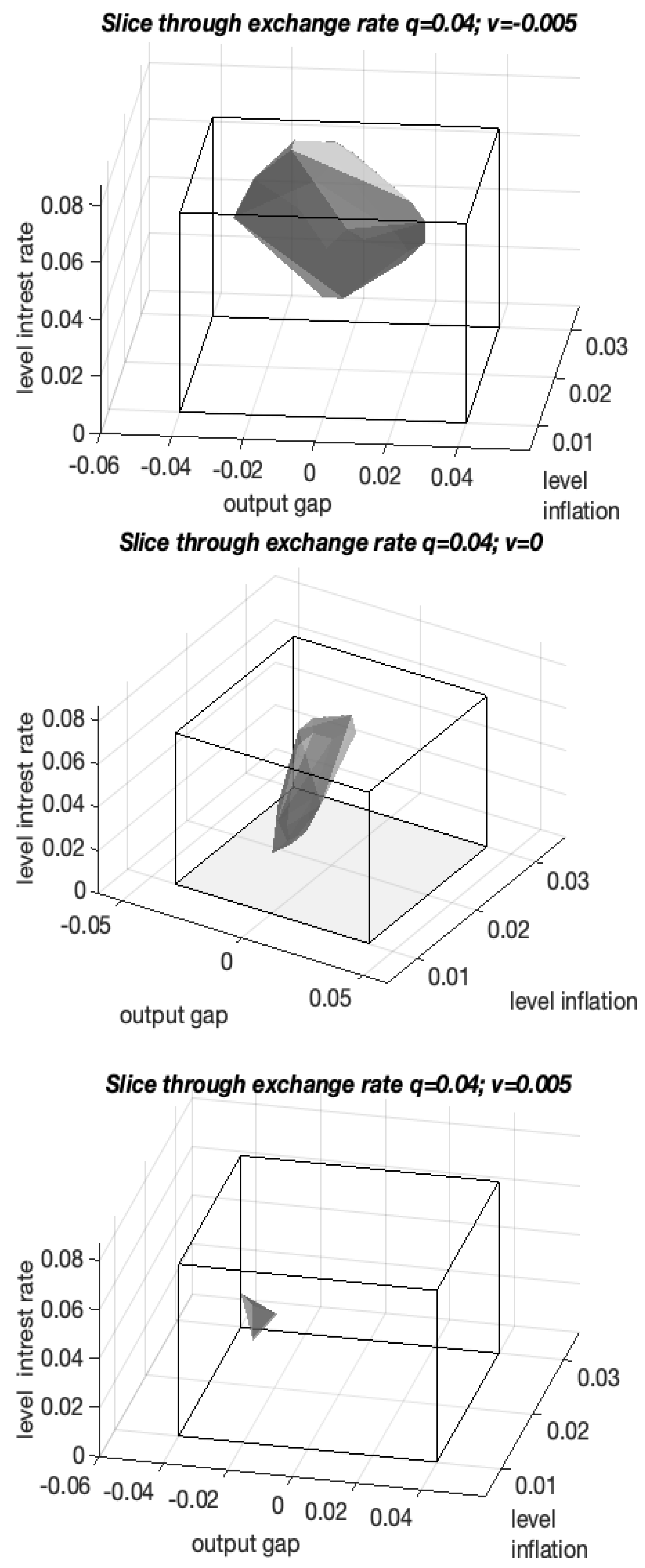
6.2. Undervalued and Overvalued Currency

Next, we study the slices through q = 0.04 (undervalued local currency) and q = 0.04 (overvalued local currency) of the computed viability kernels for v = 0.005 , v = 0 and for v = 0.005 . These are shown in Figure 6 and Figure 7, respectively. We conclude this section with a policy suggestion that the domestic bank should follow in its qualitative NA-game against the foreign bank.
The kernel slices contain all states that would enable the economy to stay in K with interest rate adjustments u U . The top panels are constructed for a negative foreign real interest rate, the middle panels are constructed a foreign real interest rate of zero, and the bottom panels are constructed for a positive foreign real interest rate. We notice that, in contrast with Figure 5, now the sizes of the boulders differ: for undervalued local currency ( q = 0.04 , left figure) the kernel slice is largest for the negative foreign real interest rate ( v = 0.005 , top panel); for overvalued local currency ( q = 0.04 , right figure) the kernel slice is largest for the positive foreign real interest rate ( v = 0.005 , bottom panel). The larger sizes indicate that the economy is viable for a bigger set of states. Therefore, the domestic bank will find it easier to cope with a negative foreign real interest rate when the exchange rate is undervalued. Correspondingly, it will be easier for the domestic bank to cope with a positive foreign real interest rate when the exchange rate is overvalued. A positive v expands the viability kernel for an overvalued currency and diminishes the kernel when the domestic currency is undervalued.
As expected, a large positive output gap is nonviable for undervalued currency, and a large negative output gap is nonviable for overvalued currency (see the middle panels). This result is consistent with the empirical observation that overvalued domestic currency depresses output.
Figure 6 and Figure 7 also give visibility to two unfavourable situations. There are few or no viable states if the domestic currency is overvalued and the foreign real interest rate is negative (see top right panel). Correspondingly, there are few or no viable states if the domestic currency is undervalued and the foreign real interest rate is positive (see bottom left panel). Although the nominal real interest rate in the US is now rising, the real interest rate is likely negative because inflation is already high. The currencies of countries such as Australia or New Zealand are probably undervalued relative to the US dollar. Therefore, these economies might be in the situation captured by the large kernel slice in the top left panel of Figure 6.
Furthermore, when examining the slices from top to bottom, we see that an increase in the foreign real interest rate pushes the slices lower. In other words, the available ranges of the domestic interest rate needed to keep the economy viable move down. This is similar to what we observed in Figure 5. In both cases, a negative v necessitates a high-interest rate to prevent output from growing too high; conversely, when v > 0 , a low-interest rate is required to keep the economy outside a liquidity trap.
The domestic bank would be ideally suited to respond to a change in the foreign interest rate by keeping the economy in the intersection of the kernels for all possible values of v V . Unfortunately, for the calibrated parameters, this intersection is an empty set. Nonetheless, the above analysis motivates our claim that the advice formulated for an economy with a neutral exchange rate, as list (a), (b) in Section 6.1, is valid for all economies. That is, the domestic bank should keep the level interest rate high if the foreign real interest rate is negative, and it should keep the level interest rate low if the foreign real interest rate is positive. Our conclusions can also be visualised with Table 1, Table 2 and Table 3. These tables show the minimum and maximum viable values of inflation, output gap and interest rate (all in level terms) for the cases of undervalued currency ( q = 0.04 ) and overvalued currency ( q = 0.04 ). They highlight the contraction of the viability kernel in situations where q and v are both positive or both negative. Furthermore, they confirm our observations that viability requires a lower domestic interest rate in order to offset a positive foreign real interest rate, and vice versa.

7. Conclusions

We have applied viability theory to a stylised macroeconomic model and explored how a central bank of a small open economy can conduct monetary policy when the foreign central bank pursues its own stabilisation policy. We have framed the problem of the domestic bank as a qualitative NA-game. To solve this problem, we have computed several viability kernels for the domestic bank, and indicated the states that enable it to preserve the viability of its economy.
It follows from our discussion on policy choices available to the domestic bank that hedging against both positive and negative foreign real interest rates seems impossible. However, if the direction of adjustment of the foreign real interest rate is known, the domestic bank may be able to establish the viability kernel. For the states in the viability kernel, there exist domestic interest rate adjustment policies that can keep the domestic economy in the desired set K.
An obvious question is what the central bank needs to do if the economy is outside the viability kernel. In such circumstances, the bank should embark on crisis control à la [35,36]. This is the approach taken by many central banks in 2022. In particular, they select their interest rate adjustments u ( t ) from a set U U (see (9)) with wider bounds u ̲ > u ̲ 1 , u ¯ > u ̲ 2 . Furthermore, the system’s dynamics can be sped up by decreasing the time intervals between adjustments. Finally, a central bank may improve the resilience of its economy to foreign shocks by expanding the viability kernel through reforms that would change the values of the coefficients a , d 2 , d 3 , p , ρ 10.

Author Contributions

Conceptualization, J.B.K. and V.P.P.; methodology, J.B.K. and V.P.P.; software, J.B.K.; validation, J.B.K. and V.P.P.; writing—original draft preparation, J.B.K.; writing—review and editing, V.P.P. All authors have read and agreed to the published version of the manuscript.

Funding

This research received no external funding.

Institutional Review Board Statement

This study did not require ethical approval.

Informed Consent Statement

Not applicable.

Data Availability Statement

All used data are explained in the paper and/or in referenced sources.

Acknowledgments

A special thank goes to Kunhong Kim our former colleague at VUW (also formerly at Hallym University in Korea) for devising the 4-variable central bank model (see Section 3.2).

Conflicts of Interest

The authors declare no conflict of interest.

Appendix A. Viable Areas

To define viable areas, viability theory introduces the viability theorem, which establishes the relationship between any closed set of points D viable under F, and the concept of the proximal normal11 to D at x. The relationship between proximal normals and the viability of D under F is defined formally in [32,47] (Theorem 2.3) and [31] (Theorem 3.2.4).
There is also an alternative, perhaps more intuitive, viability characterisation based on contingent cones. The contingent cone at x ¯ fr D (boundary of D) is the set of all directions pointing “into” D at x ¯ that form acute angles with a tangent to D at x ¯ .12 Given system’s dynamics F ( · ) , whenever it is possible to identify a closed set D such that the “velocities” F ( · ) available at x D and the directions from the contingent cone of D at x intersect, then every x D must be viable under F. In other words, there exists at least one direction in the “velocities” set F ( · ) “pointing” inside D. That is, there must exist a trajectory starting from each x D that remains in D.
Formally, the largest viability domain is the viability kernel  V F ( K ) , see (5).
For a control problem, the existence of the viability kernel V F ( K ) indicates an area for which sufficient control exists to maintain the system within V F ( K ) from any point in V F ( K ) . In other words, we know that if a trajectory begins inside the viability kernel V F ( K ) then we have sufficient controls to keep this trajectory in the constraint set K for all t. Alternatively, if evolution of the system begins outside the kernel i.e., x 0 K \ V F ( K ) , then it leaves K in finite time. When F represents the system’s dynamics of a control problem, establishing the viability kernel V F ( K ) has important implications for policy-making. In particular, it allows us to construct control rules that maintain the system’s viability, see [30].

Appendix B. Exchange Rate Responsiveness to Interest Rate Adjustments
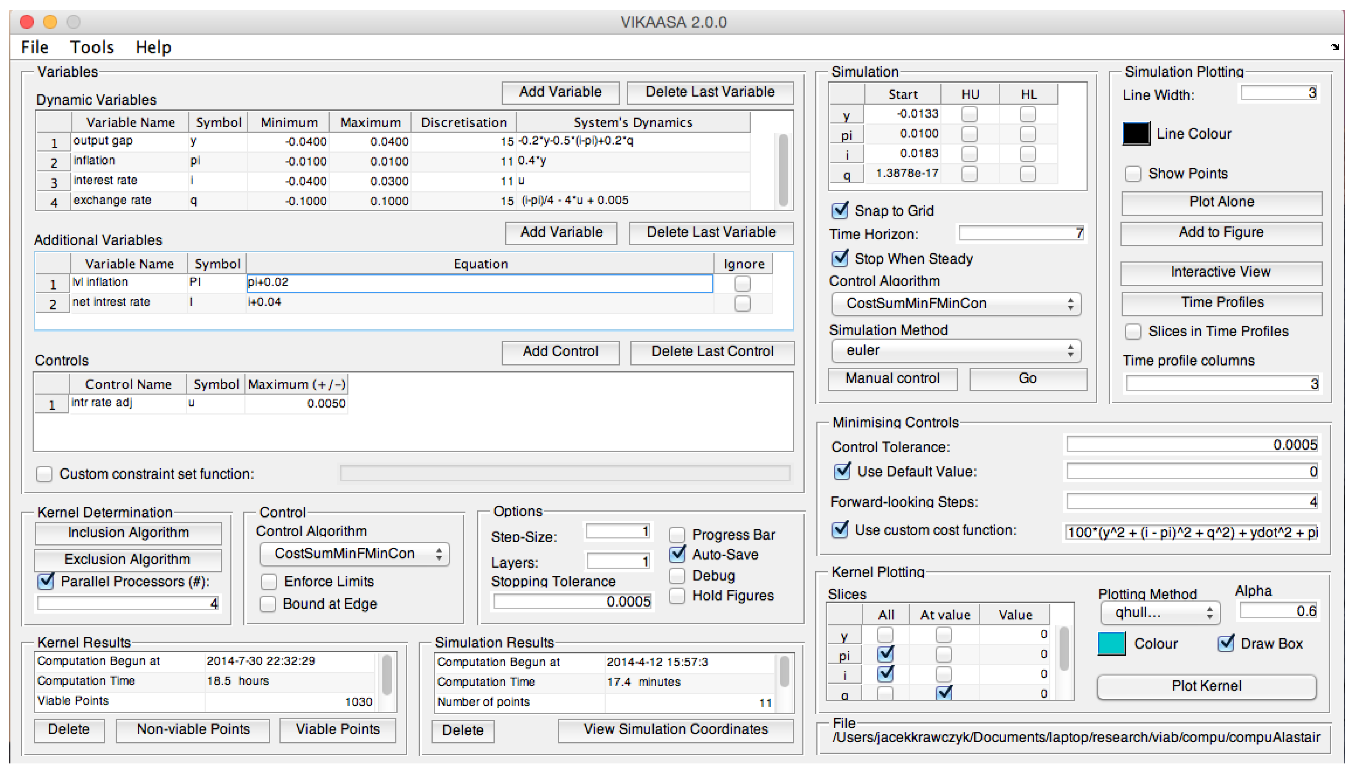
Our calibration of ρ is based on observations related to the hike in New Zealand’s interest rate by 0.25 % on 12 June 2014. Let us denote Δ i = 0.0025 . This hike was accompanied by an appreciation of the domestic currency of ( 0.8606 0.8530 ) / 0.8530 = 0.0089 1 % vis-a-vis the US dollar on the same day. We say Δ q = 0.01 .
Hence, Δ q Δ i = 0.01 0.0025 = 4 . I.e., we contend that every (positive) percentage point of change in i adds 4 points to the velocity of q measured on the day the interest rate was changed.
However, all velocities in the model (20)–(23) are expressed in 1 quarter units. We know that the exchange rate adjustments are very fast, and the period over which q can change may be very short. To make the size of ρ compatible with the other model parameters it will be assumed that there are no other interest rate changes within a quarter after the observed hike. E.g., assuming the domestic and foreign real interest rates differential is 0, the jump in i at time t will modify the value of q ( t + 1 quarter ) as follows
q ( t + 1 quarter ) q ( t ) = ρ Δ i · 1 quarter i . e . , for Δ i = 0.0025 ,
q ( t + 1 quarter ) q ( t ) = 4 · 0.0025 = 0.01 .
To summarise, we set ρ to 4. This value was also used in [10].

Appendix C. VIKAASA

VIKAASA is a specialised MATLAB application that can compute viability kernel approximations for rectangular constraint and control sets.13
VIKAASA can be used either as a set of MATLAB functions,14 or via a graphical user interface (GUI), as in Figure A1. Using the GUI one can specify the viability problem for which to the kernel is sought, run the kernel approximation algorithms and view the results. VIKAASA also supports saving and viability kernel data into files.
Figure A1. VIKAASA main interface.
Games 13 00058 g0a1
A manual for VIKAASA can be found in [45].

Notes

1
This paper draws from [1].
2
In the two-person game context, we cannot use the gender-neutral pronoun their to describe a singular player action. Instead, we will use he and his to refer to a single genderless agent.
3
For more interpretations of (3) see e.g., [30]).
4
Viability is normally defined for an infinite time horizon, but it is also possible to define Θ [ 0 , T ] , T R + , and consider viability in finite-time.
5
The parameter notation is chosen to reflect some compatibility of our model with Batini-Haldane’s discrete-time model in [39].
6
This is the reason we refer to our game as a nuisance agent game.
7
This algorithm (called the inclusion algorithm, see [9]) employed by VIKAASA will miss any viable points that cannot reach a steady state; e.g., because they form (large) orbits. However, experimenting with our monetary policy models, which consisted of using different discretisation grids and trying various controls did not lead to the discovery of points like that.
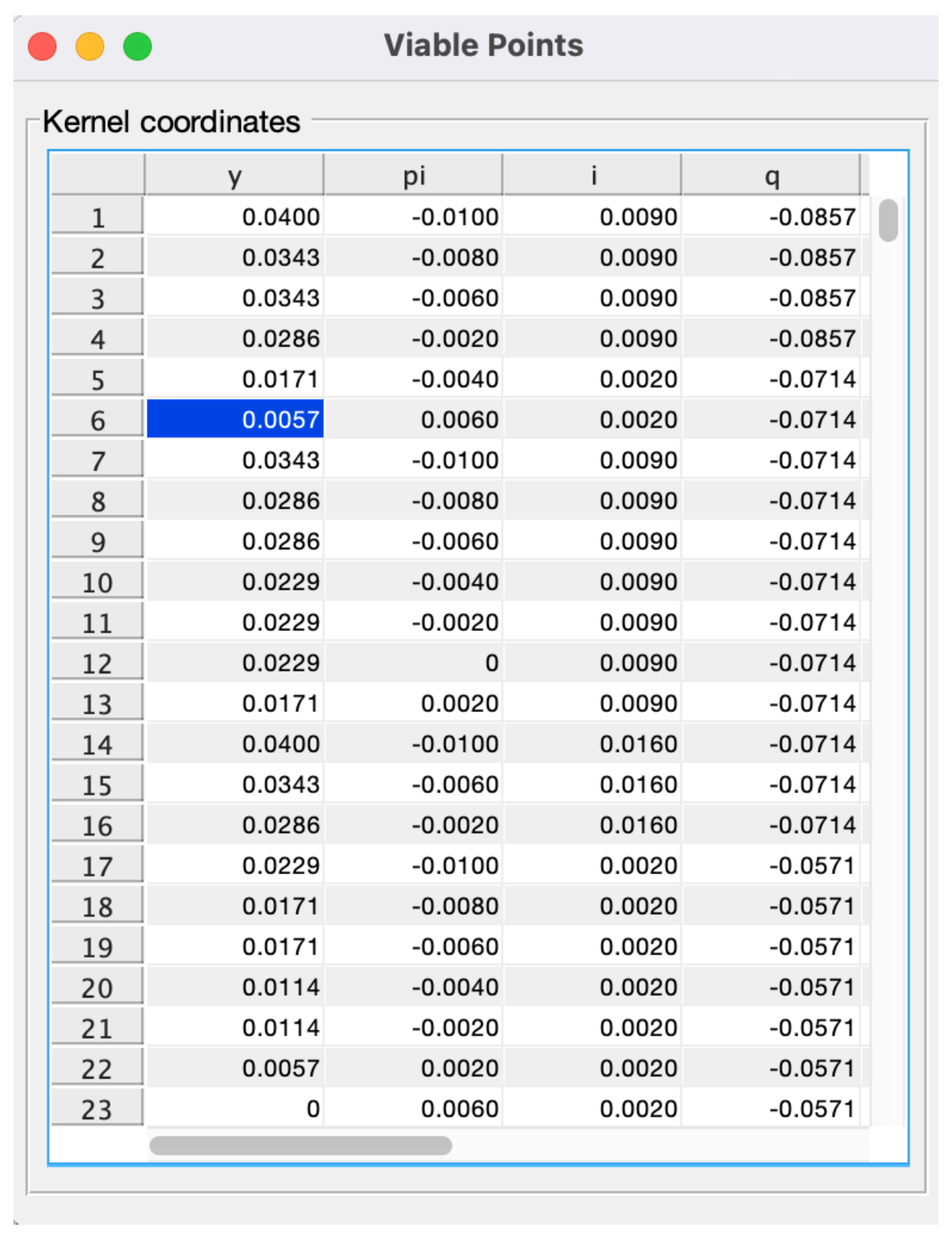
8
The total number of rows of the array for the selected discretisation (see Appendix C) is 683.
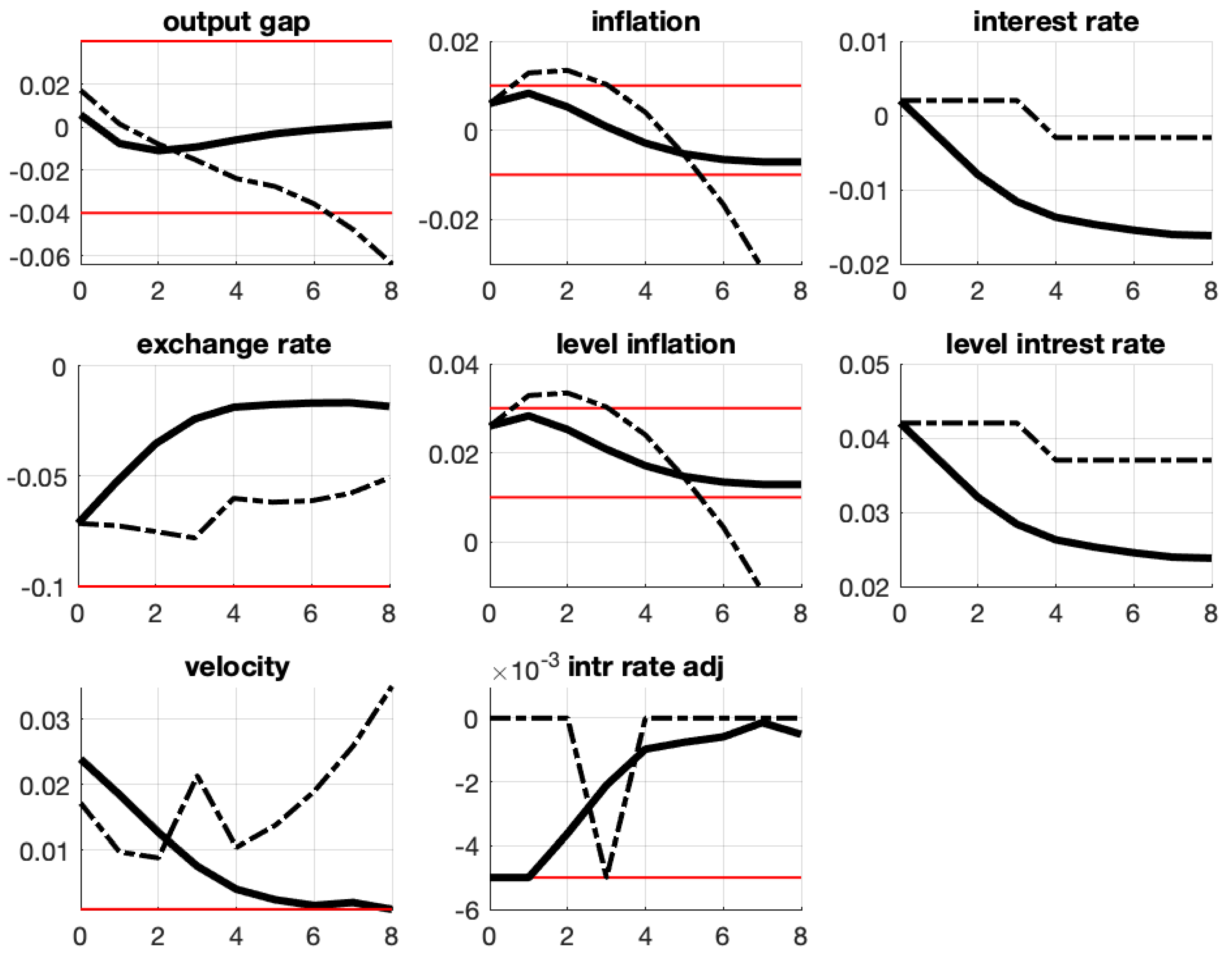
9
The penultimate subplot is the economy’s velocity norm, i.e., the sum of absolute values of the right-hand sides of (20)–(23). We consider this number a measure of an aggregate system’s velocity and call it velocity in the figure. If this velocity is close to zero, the economy has approached a steady state. If the steady-state is inside V F K and no state variable has ever breached the bounds of K then the evolution starting point is viable; refer to Appendix C.
10
See [37] for a discussion on building systemic resilience in the context of viability theory.
11
Let NP D ( x ) denotes the set of proximal normals to D at x i.e., the set of p R n such that the distance of x + p to D is equal to | | p | | .
12
If D were a disc, then a contingent cone at any point of the circumference would be a half-space. When x ¯ is an interior point of D, then the contingent cone for this point is the whole space.
13
VIKAASA stands for Viability Kernel Approximation, Analysis and Simulation Application = VIKAASA, which happens to be a Sanskrit word that means “progress” or “development”.
14
VIKAASA is also compatible with GNU Octave, but without the GUI. See the manual for more information.

References

  1. Krawczyk, J.B.; Kim, K. An analysis of monetary policy of a small open economy with a ‘nuisance’ agent. In Proceedings of the Conference Maker, 20th International Conference on Computing in Economics & Finance, Oslo, Norway, 22–24 June 2014. [Google Scholar]
  2. Cardaliaguet, P.; Quincampoix, M.; Saint-Pierre, P. Set valued numerical analysis for optimal control and differential games. In Stochastic and Differential Games. Annals of the International Society of Dynamic Games; Birkhäuser: Boston, MA, USA, 1999; Volume 4, pp. 177–274. [Google Scholar]
  3. Hertwig, R.; Hoffrage, U. Simple Heuristics in a Social World; Oxford University Press: Oxford, UK, 2013. [Google Scholar]
  4. Beckenkamp, M. Playing Strategically against Nature?—Decisions Viewed from a Game-Theoretic Frame; MPI Collective Goods: Bonn, Germany, September 2008. [Google Scholar]
  5. Hansen, L.P.; Sargent, T.J.; Turmuhambetova, G.; Williams, N. Robust control and model misspecification. J. Econ. Theory 2006, 128, 45–90. [Google Scholar] [CrossRef]
  6. Dennis, R.; Leitemo, K.; Söderström, U. Methods for robust control. J. Econ. Dyn. Control 2009, 33, 1604–1616. [Google Scholar] [CrossRef]
  7. Dennis, R.; Leitemo, K.; Söderström, U. Monetary Policy in a Small Open Economy with a Preference for Robustness; Working Paper 2007-04; Federal Reserve Bank of San Francisco: San Francisco, CA, USA, 2009. [Google Scholar]
  8. Žaković, S.; Rustem, B.; Wieland, V. A Continuous Minimax Problem and its Application to Inflation Targeting. In Decision and Control in Management Science; Zaccour, G., Ed.; Kluwer Academic Publishers: Dordrecht, The Netherlands, 2002. [Google Scholar]
  9. Krawczyk, J.B.; Pharo, A.; Serea, O.S.; Sinclair, S. Computation of viability kernels: A case study of by-catch fisheries. Comput. Manag. Sci. 2013, 10, 365–396. [Google Scholar] [CrossRef]
  10. Krawczyk, J.B.; Kim, K. Viable stabilising non-Taylor monetary policies for an open economy. Comput. Econ. 2014, 43, 233–268. [Google Scholar] [CrossRef]
  11. Aubin, J.P.; Bayen, A.M.; Saint-Pierre, P. Viability Theory: New Directions, 2nd ed.; Springer: Berlin, Germany, 2011. [Google Scholar] [CrossRef]
  12. Aubin, J.P.; Da Prato, G.; Frankowska, H. Set-Valued Analysis; Springer: Berlin, Germany, 2000. [Google Scholar]
  13. Krawczyk, J.B.; Kim, K. “Satisficing” Solutions to a Monetary Policy Problem: A Viability Theory Approach. Macroecon. Dyn. 2009, 13, 46–80. [Google Scholar] [CrossRef]
  14. The Economist. Why the Federal Reserve Has Made a Historic Mistake on Inflation. The Economist, 23 April 2022. [Google Scholar]
  15. Krawczyk, J.B.; Sethi, R. Satisficing Solutions for New Zealand Monetary Policy; Technical report, Reserve Bank of New Zealand, No DP2007/03; Reserve Bank of New Zealand: Wellington, New Zealand, 2007.
  16. Béné, C.; Doyen, L.; Gabay, D. A viability analysis for a bio-economic model. Ecol. Econ. 2001, 36, 385–396. [Google Scholar] [CrossRef]
  17. De Lara, M.; Doyen, L.; Guilbaud, T.; Rochet, M.J. Is a management framework based on spawning stock biomass indicators sustainable? A viability approach. ICES J. Mar. Sci. 2007, 64, 761–767. [Google Scholar] [CrossRef]
  18. Martinet, V.; Doyen, L. Sustainability of an economy with an exhaustible resource: A viable control approach. Resour. Energy Econ. 2007, 29, 17–39. [Google Scholar] [CrossRef]
  19. Martinet, V.; Thébaud, O.; Doyen, L. Defining viable recovery paths toward sustainable fisheries. Ecol. Econ. 2007, 64, 411–422. [Google Scholar] [CrossRef] [Green Version]
  20. Pujal, D.; Saint-Pierre, P. Capture Basin Algorithm for Evaluating and Managing Complex Financial Instruments. In Proceedings of the 12th International Conference on Computing in Economics and Finance, Limassol, Cyprus, 22–24 June 2006. [Google Scholar]
  21. Krawczyk, J.B.; Sissons, C.; Vincent, D. Optimal versus satisfactory decision making: A case study of sales with a target. Comput. Manag. Sci. 2012, 9, 233–254. [Google Scholar] [CrossRef]
  22. Clément-Pitiot, H.; Doyen, L. Exchange Rate Dynamics, Target Zone and Viability; Université Paris X Nanterre: Nanterre, France, 1999. [Google Scholar]
  23. Krawczyk, J.B.; Kim, K. A Viability Theory Analysis of a Macroeconomic Dynamic Game. In Proceedings of the Eleventh International Symposium on Dynamic Games and Applications, Tucson, AZ, USA, 4 December 2004. [Google Scholar]
  24. Clément-Pitiot, H.; Saint-Pierre, P. Goodwin’s models through viability analysis: Some lights for contemporary political economics regulations. In Proceedings of the 12th International Conference on Computing in Economics and Finance, Limassol, Cyprus, 22–24 June 2006. [Google Scholar]
  25. Bonneuil, N.; Saint-Pierre, P. Beyond Optimality: Managing Children, Assets, and Consumption over the Life Cycle. J. Math. Econ. 2008, 44, 227–241. [Google Scholar] [CrossRef]
  26. Bonneuil, N.; Boucekkine, R. Viable Ramsey economies. Can. J. Econ./Revue Can. D’économique 2014, 47, 422–441. [Google Scholar] [CrossRef]
  27. Krawczyk, J.B.; Judd, K.L. A note on determining viable economic states in a dynamic model of taxation. Macroecon. Dyn. 2016, 20, 1395–1412. [Google Scholar] [CrossRef]
  28. Kim, K.; Krawczyk, J.B. Sustainable Emission Control Policies: Viability Theory Approach. Seoul J. Econ. 2017, 30, 291–317. [Google Scholar]
  29. Krawczyk, J.B.; Serea, O.S. When can it be not optimal to adopt a new technology? A viability theory solution to a two-stage optimal control problem of new technology adoption. Optim. Control Appl. Methods 2013, 34, 127–144. [Google Scholar] [CrossRef]
  30. Krawczyk, J.B.; Pharo, A. Viability theory: An applied mathematics tool for achieving dynamic systems’ sustainability. Math. Appl. 2013, 41, 97–126. [Google Scholar]
  31. Aubin, J.P. Viability Theory; Systems & Control: Foundations & Applications; Birkhäuser: Boston, MA, USA, 1991. [Google Scholar] [CrossRef]
  32. Quincampoix, M.; Veliov, V.M. Viability with a target: Theory and Applications. In Applications of Mathematics in Engineering; Heron Press: Rubery, UK, 1998; pp. 47–58. [Google Scholar]
  33. Veliov, V.M. Sufficient conditions for viability under imperfect measurement. Set-Valued Anal. 1993, 1, 305–317. [Google Scholar] [CrossRef]
  34. Simon, H.A. A Behavioral Model of Rational Choice. Q. J. Econ. 1955, 69, 99–118. [Google Scholar] [CrossRef]
  35. Martinet, V.; Thébaud, O.; Rapaport, A. Hare or Tortoise? Trade-offs in Recovering Sustainable Bioeconomic Systems. Environ. Model. Assess. 2010, 15, 503–517. [Google Scholar] [CrossRef]
  36. Doyen, L.; Saint-Pierre, P. Scale of viability and minimal time of crisis. Set-Valued Anal. 1997, 5, 227–246. [Google Scholar] [CrossRef]
  37. Karacaoglu, G.; Krawczyk, J.B. Public policy, systemic resilience and viability theory. Metroeconomica 2021, 72, 826–848. [Google Scholar] [CrossRef]
  38. Isaacs, R. Differential Games; Wiley: New York, NY, USA, 1965. [Google Scholar]
  39. Batini, N.; Haldane, A. Monetary policy rules and inflation forecasts. In Bank of England Quarterly Bulletin; Bank of England: London, UK, 1999. [Google Scholar]
  40. Walsh, C. Monetary Theory and Policy; MIT Press: Boston, MA, USA, 2003. [Google Scholar]
  41. Svensson, L. Open-economy inflation targeting. J. Int. Econ. 2000, 50, 155–183. [Google Scholar] [CrossRef]
  42. Eaton, J.; Turnovsky, S.J. Covered Interest Parity, Uncovered Interest Parity and Exchange Rate Dynamics. Econ. J. 1983, 93, 555–575. [Google Scholar] [CrossRef]
  43. Batini, N.; Haldane, A. Forward-looking rules for monetary policy. In Monetary Policy Rules; Taylor, J.B., Ed.; National Bureau of Economic Research: Cambridge, MA, USA, 1999; pp. 157–202. [Google Scholar] [CrossRef]
  44. Gaitsgory, V.; Quincampoix, M. Linear Programming Approach to Deterministic Infinite Horizon Optimal Control Problems with Discounting. SIAM J. Control Optim. 2009, 48, 2480–2512. [Google Scholar] [CrossRef]
  45. Krawczyk, J.B.; Pharo, A. Manual of VIKAASA 2.0: An Application for Computing and Graphing Viability Kernels for Simple Viability Problems; SEF Working Paper 08/2014; Victoria University of Wellington: Wellington, New Zealand, 2014. [Google Scholar]
  46. Krawczyk, J.B.; Pharo, A.S. Viability Kernel Approximation, Analysis and Simulation Application—VIKAASA Code. 2014. Available online: https://github.com/socsol/vikaasa (accessed on 17 August 2022).
  47. Cardaliaguet, P.; Quincampoix, M.; Saint-Pierre, P. Set-Valued Numerical Analysis for Optimal Control and Differential Games. Ann. Int. Soc. Dyn. Games 1999, 4, 177–247. [Google Scholar] [CrossRef]
Figure 1. The viable and non viable trajectories for a time-invariant dynamic system.
Games 13 00058 g001
Figure 2. Viable points (fragment).
Games 13 00058 g002
Figure 3. Time profiles of economy evolutions.
Games 13 00058 g003
Figure 4. Economy evolutions shown in 3D spaces.
Games 13 00058 g004
Figure 5. Slices of the viability kernel for neutral exchange rate when v = 0.005 , v = 0 and v = 0.005 .
Games 13 00058 g005
Figure 6. Viability kernels for undervalued currency.
Games 13 00058 g006
Figure 7. Viability kernels for overvalued currency.
Games 13 00058 g007
Table 1. Minimum and maximum viable values of inflation, output gap and interest rate (all in level terms) for v = 0.005 .
π min π max y min y max i min i max
q = 0.04 0.010.020.0230.040.0560.07
q = 0.04 0.010.03−0.0340.0280.0350.07
Table 2. Minimum and maximum viable values of inflation, output gap and interest rate (all in level terms) for v = 0 .
π min π max y min y max i min i max
q = 0.04 0.010.03−0.0160.0320.0350.056
q = 0.04 0.010.03−0.0320.0080.0210.042
Table 3. Minimum and maximum viable values of inflation, output gap and interest rate (all in level terms) for v = 0.005 .
π min π max y min y max i min i max
q = 0.04 0.010.03−0.0290.0290.0070.042
q = 0.04 0.0220.03−0.04−0.0230.0140.021
Publisher’s Note: MDPI stays neutral with regard to jurisdictional claims in published maps and institutional affiliations.

