1. Introduction
Immunotherapy is a method of cancer treatment, in which the immune system is used to fight the tumor. The immune system protects the body from infections and diseases. It attacks pathogens such as bacteria and viruses. The immune system also helps to get rid of the body’s diseased or damaged cells. The basic idea of immunotherapy is simple: to help the body protect itself from malicious “invaders”. However, cancer cells can be insidious. Often, they find a way to “hide” from the immune system or to disable its response. In general, immunotherapy aims to counteract some of these ways of evading immune system attacks: helps the immune system find cancer cells and to kill them. There are different types of immunotherapy, each of which has its own mechanism to strengthen the immune system’s response.
One of the encouraging ways to use the body’s capabilities in the fight against cancer is therapy with so-called T-lymphocytes with chimeric antigen (antigens—substances foreign to the body that cause its immune response) receptors, abbreviated CAR-T, (Chimeric Antigen Receptor T-cell) appeared relatively recently, at the beginning of the 21th century. In numerous publications this therapy is called “a breakthrough in the treatment of oncology”, “a new era in medicine” [
1,
2].
What is the idea behind such a molecule? One of its parts recognizes markers on the surface of the tumor cell, while other parts transmit an activating signal to the cell of the immune system to destroy the tumor cell. CAR T-cells are produced in the following way: T-lymphocytes are extracted from the patient’s blood, that is, cells that should normally protect us from cancer and virus-infected cells. This is done through apheresis, a technology that separates blood into components and produces a certain number of lymphocytes. Then, DNA encoding CAR is inserted into the chromosomes of T-lymphocytes, and the cell begins to produce on its surface those very chimeric, that is, artificially created receptors that do not exist in nature. They are designed so that T-lymphocytes find markers on the surface of cancer cells and receive a signal to attack them. The thus obtained CAR T-cells are expanded and injected back into the patient’s blood.
What happens next? If CAR T-cells in a patient’s body collide with a normal cell, they are supposed to simply float past each other; if they find a cancer cell, the chimeric antigen receptor recognizes a specific marker on it, to which it was tuned during creation. The T-lymphocyte kills the cancer cell and starts dividing very actively. One cell, equipped with a CAR T-receptor, produces hundreds and even thousands. Such a self-replicating medicine. It was a believe that as long as there are cancer cells in some corners of the body, CAR T-lymphocytes will destroy them. When all cancer cells are destroyed, most of the CAR T-cells will die, some will remain in the bone marrow to reappear, multiply and destroy the cancer if they recur. Why, then, even in the best case, the effectiveness of treatment is only 50–90%, not
? ([
2], table 2) It was found that
of cancer cells can carry the target that CAR T-lymphocytes are targeting, but
cannot. And these
remain intact in the body and multiply. In addition, some cancer cells can “escape” from CAR T-lymphocytes if it “removes” or modifies targets on the surface of its cells. There are other problems that complicate treatment with chimeric antigen receptors. For example, despite the fact that CAR T-cells by themselves can live a long time, in an organism depleted by multiple chemotherapy they will multiply rather sluggishly and ineffectively fight cancer cells. This is partly why this approach does not work in all cases.
At the same time, these antigens are not strictly cancer specific. When immunotherapy emerged as an alternative to radio and chemotherapy, many people thought that this method of treatment was not as harmful for the patients. However, CAR, although the most expensive, is still in the process of developing because modified lymphocytes also kill healthy cells [
3]. For example, in the immune therapy used in treating blood cancers, CAR T-cells target CD19 antigen that is also found on normal B-lymphocytes [
4]. So, anti-CD19 CAR therapy leads to a decrease in blood of B-lymphocytes (B-cell aplasia), which should be justified by the clinical anticancer effect in each particular case [
5,
6]. Thus, the current chimeric T-cell receptors are not strictly specific to cancer cells. In this regard, there may be a toxic effect on the principle of “organ-transplant against the host” [
7,
8,
9]. In some cases, as is the case with B-cell aplasia in the treatment of anti-CD19 CAR T-lymphocytes of lympho-proliferative diseases, this is not too severe a complication and is stopped by the introduction of immunoglobulin [
2]. However, sometimes the toxic effect of CAR T-lymphocytes is an obstacle to their clinical use. Everything is determined by the correctness of the chosen target and the acceptable level of observed complications [
10].
The world has already conducted clinical trials on several thousand patients with blood cancers. The FDA (Food and Drug Administration) approved the first application of CD19 CAR immunotherapy for USA patients in 2007. Now this therapy shows the effectiveness of 50–90% in the treatment of patients even with terminal stage lymphoblastic leukemia, lymphoma and myeloma [
2]. Side effects are associated with the fact that CAR T-cells are too powerful. By attacking cancer cells, they also affect other cells of the immune system, forcing them to release massively biologically active substances, cytokines. This leads to another major problem in the usage of CAR lymphocytes, the so-called “cytokine storm”.
The symptom of “a cytokine storm” is primarily an increase in temperature and hypotension, which can lead to multiple organ failure. The prevention of it consists of the use of steroids, vasopressors and supportive therapy in the conditions of the intensive care unit. Recently, the use of antibodies against TNF-
(infliximab) and antibodies against the interleukin-6 receptor (tocilizumab) or monotherapy with the use of tocilizumab showed good results (see, for example, [
11]). Unlike many conventional drug-induced side effects, this toxicity cannot be managed by simply reducing the dosage of the drug, as the number of proliferating T-cells will increase in number and may eventually reach critical level. Prevention of the “cytokine storm” is seems to be manageable by the fractional introduction of T-lymphocytes or by the use of short-lived populations of lymphocytes [
10]. It is gratifying that many doctors have already learned to predict and control the development of “a cytokine storm” in most patients.
Thus, besides the purely biomedical task of making immunotherapy more specific to certain types of cancer, there are two main questions with CAR T-cell immunotherapy:
With what frequency and at what intervals should chimeric leukocytes be injected and in what concentrations?
How to take a medicine that suppresses the “surge” of the immune system? If between injections the patient seems to be resting, is it necessary to simultaneously stop giving the immunosuppressant, or are these two independent procedures?
In order not to go through all the possible options in the treatment of cancer patients, one can try to formulate the situation in immunotherapy mathematically and create a mathematical model to answer these and other questions. Currently, many models have been created that help to understand and predict both the dynamics of tumor growth itself and those works whose authors propose controlled models and, together with optimization ideas, simultaneously try to find the optimal treatment protocol. In this sense, the survey of mathematical models for leukemia and lymphoma given in [
12] is very useful. It shows that deterministic ODE models can serve as good approximations of the average behavior of a system when the populations are large and so such models can be suitable for describing the late stages of cancer.
The main goal of mathematical modeling of cancer is to improve treatment, either by optimizing the way existing therapies are being administered or by motivating novel therapies [
12]. After consideration of many papers, we find especially interesting the works of [
13], in which the authors present a competition model of cancer tumor growth that includes the immune system response and drug therapy, as well as a recent article [
14], in which the authors model chimeric anti-gene receptor T-cell therapy (CAR therapy) with presence of interleukin-6, the cytokine responsible for “cytokine storm”. In both papers the authors use the optimal control theory to numerically find the optimal treatment schedule.
For various reasons, as well as depending on the individual characteristics of the patient undergoing immunotherapy treatment, chimeric cells can behave ambiguously or differently: they either become too active and divide uncontrollably, or vice versa, behave sluggishly, inactive, sometimes killing healthy cells. It seems logical to model the case of super-active CAR T-cells either with a predator-one prey model plus additional competition between healthy and cancer cells (this would be a case of ideal immunotherapy) or with a model with one predator and two preys (this is when active chimeras are nonspecific and might kill healthy cells as well). In turn, for an organism weakened by radio- or chemotherapy, CAR T-cells are not very active or specific and the competition model for all three types of cells seems more suitable. The model of the latter type is considered in this work, which is the continuation of our studies presented in [
15,
16,
17].
We propose and investigate controlled model of CAR T-cell immunotherapy that employs and combines the best ideas presented in [
13,
14]. In our controlled model, the dynamics of CAR T-cells, normal or healthy B-cells, cancer cells, and the cytokines is described by four ordinary differential equations of Lotka-Volterra competition type with two bounded controls. The first control represents the concentration of the injected CAR immune T-cells and its influence on the variables of system. The second control reflects the effect of the immunosuppressant drug, such as tocilizumab and its role on preventing “cytokine storm”.
The paper is organized as follows. In
Section 2 we define the model and state the optimal control problem of minimizing the tumor’s cells and concentration of the cytokines. In
Section 3, we apply the Pontryagin maximum principle and find the type of optimal controls that depend on the switching functions. Here we find that the second optimal control reflecting the suppressive effect of possible “cytokine storm” is constant, taking the maximum value on the entire time interval of treatment period. In
Section 4, we study the properties of the first switching function analytically and find that the corresponding optimal control takes its maximum value in the end of the time interval. In
Section 5,
Section 6 and
Section 7, we reduce the matrix to an upper triangular form, split the system and analyze quadratic subsystems. In
Section 8, we find the type of the switching function that determines the behavior of the first optimal control responsible for the CAR injection schedule. We prove that the switching function has not more than two zeros. In
Section 9 we find analytically that the first optimal control has at most two switchings and that depending on model parameters, it can take one of the five optimal treatment scenarios.
Section 10 shows computer simulation of the model at different model parameters and demonstrate the optimal solutions.
Section 11 contains our conclusions.
2. Model and Optimal Control Problem
At a given time interval
, which is the treatment time, let us consider a controlled model for the spread and immunotherapy of leukemia. The model is described by the following nonlinear system of differential equations:
with given initial values:
In this model, denotes the population of CAR modified T-lymphocytes at time t, the population of B-leukemic or cancer cells, the population of healthy B-cells, and —inflammatory cytokines, such as Il-6, the population of which is elevated by the immune therapy.
Firstly, let us consider the second and the third equations of the control system. The first two terms of the both equations:
reflect a logistic growth law for the cancer and healthy B-cells. The parameters
p,
q and
,
represent the corresponding per capita growth rates and reciprocal carrying capacities of these types of cells. The last terms in the both equations
and
represent decrease in the populations of the cancer and healthy cells because of their competition;
and
are the corresponding competition coefficients. The third terms in the both equations
and
show a decrease in the populations of cancer and healthy cells as a result of their interaction with the immune modified T-cells,
. Here,
and
are the corresponding relative compatibility coefficients.
Secondly, let us explain the first and the fourth equations of the model. In the first equation, the first term
involves proliferation of CAR T-cells due to stimulation by encounters with their target cells that contain CD19 antigen, and
r is the per capita growth rate of this type of cells. We do not consider here their natural death since they do not undergo apoptosis after killing the target cells [
3]. While the
cells population does decrease after killing the target cells,
,
that is displayed by the corresponding second and third terms
and
of the first differential equation, this interaction with target cells somewhere how stimulates CAR cells proliferation. Here
and
are the corresponding killing efficiency of CAR T-cells in relation to cancer and healthy cells. The last term
of the first equation reflects an increase in the population of
cells due to the controlled injection of the modified chimeric T-cells. Here
is the first bounded control. This control represents a kind of intensity of CAR immunotherapy. The control itself changes from zero to the maximum value. If the control is equal to zero, then the injection of chimeric cells is not performed, and if it is maximum, then this corresponds to the injection with the maximum concentration of chimeric cells. The mathematical properties of control
are explained below. Finally,
m reflects the efficiency of the CAR T-cell therapy.
The fourth differential equation describes the dynamics of the Il-6 cytokines. The first term
of it is the influx rate (secreting rate) of the cytokines. The second term
indicates a negative feedback mechanism mentioned in [
14], and
is the cytokine decay rate. An elevating increase in the cytokine level caused by the CAR T-cell immunotherapy that appears as the “cytokine storm”, manifested as a systemic inflammatory process in all vital organs of patients receiving CAR immunotherapy, is reflected by the last term
of the differential equation. This last term of the controlled model contains the second bounded control
that plays the role of the intensity of the dosage of immunosuppressant drug intake. The second bounded control takes values from 0 (no medication is given) to 1 (the maximum dosage of anti-inflammatory drag is taken), and
n reflects the efficiency of this dosage. Our goal is by using two controls, find such optimal treatment protocol that minimizes the cancer cells and prevent over activity of the cytokines.
All the parameters of the model are positive constants, the value of which depends on each specific case. We consider that the following assumption is true.
Assumption 1. Let in system (
1)
the parameters: r, p, q, m, n, η, γ, λ, ν, , , , , , be positive, and for them the following inequalities hold:and one of the inequalities in (
3)
and in (
5)
be strict. It is easy to see that the fulfillment of inequalities (
3)–(
5) implies the validity of the following relationships:
Next, in system (
1), two control functions
and
are introduced. They subject to the restrictions:
We consider that the set of all admissible controls
is formed by all possible pairs of Lebesgue measurable functions
, which for almost all
satisfy inequalities (
8).
The positiveness, boundedness and continuation of the solutions for system (
1) and (
2) is established by the following lemma.
Lemma 1. For any pair of admissible controls the corresponding absolutely continuous solutions , , , for system (
1)
and (
2)
are defined on the entire interval and satisfy the inequalities:where The proof of Lemma 1 is fairly straightforward and we omit it.
Now, let us consider for system (
1) and (
2) on the set of admissible controls
the following minimization problem:
where
and
are positive weighting factors. The objective function in (
10) is a sum of terminal and integral parts. The terminal part reflects the patient’s state (the weighted combination of the populations of leukemia cells, healthy B-cells and cytokines) at the end of the treatment period, and the integral term sets this state throughout the entire treatment period. For convenience of notation, in the objective function we denote the terminal part by
I.
The existence in the minimization problem (
10) of the optimal controls
and the corresponding optimal solutions
,
,
,
for system (
1) and (
2) follows from Lemma 1 and Theorem 4 ([
18], Chapter 4). Indeed, the key assumptions of this theorem are true. Namely, inequalities (
9) from Lemma 1 give a uniform estimate for the solution
of system (
1) and (
2) corresponding to any pair of admissible controls
from
for all
. This is the first key assumption. Next, system (
1) is linear in controls
and
, and the integrand of the objective function in (
10) does not depend on these controls. These facts ensure the convexity of the set of generalized velocities, which is the second key assumption.
4. Properties of the Switching Functions and Optimal Controls
We establish the validity of the following lemma.
Lemma 2. The adjoint variable is negative on the interval .
Proof of Lemma 2. Let us select from the adjoint system (
11) the Cauchy problem for the adjoint variable
in the form
and then integrate it. As a result, we find the formula
from which the statement of this lemma immediately follows. □
The validity of the theorem below follows from Lemmas 1 and 2 and also Formula (
13).
Theorem 1. Optimal control is a constant function of the type This fact means that the drug intake, which is given by the control function , occurs with maximum intensity of 1 over the entire treatment period .
Now we substitute the Formula (
14) into the first equation of the adjoint system (
11), and also exclude the last equation from it together with the corresponding initial condition. As a result, we obtain the simplified adjoint system:
In this system, let us perform the change of adjoint variables in accordance with the formulas:
Due to the corresponding equations of systems (
1) and (
15), we obtain appropriate equations for the new adjoint variables (
16) as
Adding to them following from (
15) and (
16) new initial conditions, we find the corresponding adjoint system:
Now, analyzing relationship (
12) and the first formula in (
16), we rewrite this relationship as follows
where
is a switching function, the behavior of which defines the form of the optimal control
.
Let us obtain the system of differential equations for the function
. We introduce the first function corresponding to the switching function as
Then, the first differential equation in (
17) can be rewritten as
where
.
By the inequalities (
5) from Assumption 1, we introduce the second function corresponding to the switching function as
Then, using the second and third equations of system (
17), we find the equation:
where the functions
,
,
are defined as
Again using the third equation of system (
17) and also the second and third equations of system (
1), we obtain the equation:
where the functions
,
,
are defined by the formulas:
and the function
is given by the relationship
By inequalities (
3) and (
5), it is easy to see that this function takes positive values on
.
Remark 1. An important property of the function is its sign-definiteness on the interval . From the analysis of the formula (
23),
we can conclude that this property is preserved if, instead of inequalities (
3),
the inequalities:hold, and only one of them is strict. Then, the function takes negative values on . Now, gathering Equations (
19), (
21) and (
22) for functions
,
,
in one system and then adding the appropriate initial conditions due to the definitions of these functions and the initial conditions from (
17), we find the required system of differential equations for the switching function
and the functions
and
that correspond to it:
with the initial conditions for the first two functions:
Here the function
is defined by Formula (
23).
Finally, let us analyze the behavior of the switching function in a neighborhood of . The following lemma is true.
Lemma 3. In the neighborhood adjacent to , the switching function takes only positive values if , and only negative values if .
Proof of Lemma 3. First, let us consider the case, when
The definition of the function
implies its continuity on the interval
. Then, the neighborhood of
is defined, in which due to (
27) and the second initial condition from (
26), this function is negative if
, and positive if
. Then, integrating in this neighborhood the first equation of system (
25) with the appropriate initial condition from (
26), we find the formula
from which the positivity or negativity of the switching function
immediately follows.
Now, we consider the case, when
It is easy to see that then the Formula (
20) implies the equality
and the initial condition from (
26) for the function
is rewritten as
. Let us integrate the second equation of system (
25) with this initial condition. As a result, we have the formula
The definitions of the functions
,
,
,
ensure their continuity on the interval
. Then, the first initial condition from (
26) and (
29) imply the existence of the neighborhood of
in which the function
takes positive values. Considering the values of
t in Formula (
30) only from this neighborhood, we conclude that in it the function
is negative. Due to (
28), we see that in this neighborhood the switching function
takes positive values. □
The validity of the theorem below follows from Lemma 3 and Formula (
18).
Theorem 2. A neighborhood is defined adjacent to , at which the optimal control takes the maximum value if , and the minimum value 0 if .
This fact means that the CAR T-cell therapy, which is expressed by the control function , at the end of the treatment period can occur with both maximum intensity and minimum intensity 0.
5. Reducing the Matrix of System to the Upper Triangular Form
We see that the system (
25) is linear non-autonomous system of differential equations. Its matrix has the form:
For the convenience of analysis of such a system, we reduce this matrix to a special upper triangular form
using a change of variables:
where the functions
,
will be determined later in a special way. In matrix (
31), the symbol * denotes its nonzero elements.
Now, let us obtain the corresponding differential equations for the functions
,
and
using the equations of system (
25). Performing direct calculations, for the function
we have the equation:
Using similar calculations for the function
, the following expression can be found
Let us choose the functions
,
in such a way that the expression for
vanishes identically. This implies that the function
satisfies the differential equation:
Then, expression (
33) is transformed to the differential equation:
Finally, we carry out similar direct calculations for the function
. As a result, the following expression can be obtained
Let us choose the functions
,
in such a way that the expressions for
and
vanish identically. This implies that the functions
and
satisfy the differential equations:
Then, expression (
36) is transformed to the differential equation:
Gathering the Equations (
32), (
35) and (
38) into one system, for the functions
,
and
we obtain the linear non-autonomous system of differential equations:
the matrix of which has the required upper triangular form (
31).
Gathering the Equations (
34) and (
37) also in one system, for the functions
,
realizing representation (
39), we have the quadratic non-autonomous system of differential equations:
Initial conditions
can be added to system (
40), where
,
and
are constants. As a result, we have the Cauchy problem (
40) and (
41). Then, as a consequence of the Existence and Uniqueness of Solution Theorem [
20], solutions
,
,
to this problem can be defined only locally, in a neighborhood of
. However, for this problem it is important to have solutions of the Cauchy problem (
40) and (
41) defined on the entire interval
(see [
21,
22,
23]). That is we have to find the restrictions on the functions
,
,
and
,
, or what is the same, on the parameters of system (
1) such that under these restrictions solutions of the Cauchy problem (
40) and (
41) are defined on the entire interval
. Then system (
39) would be also defined on the entire interval, and hence, it would be possible to use the Generalized Rolle’s Theorem [
24] to estimate the number of zeros of the switching function
.
7. Analysis of Quadratic Subsystems
Let us analyze the quadratic subsystems (
42) and (
47). For this, we will assume that the solutions
,
of system (
47) and the solutions
,
of system (
42) are determined on the maximal intervals of existence of such solutions [
18,
20]: specifically, we assume that functions
and
are determined on the interval
, and functions
and
are determined on the interval
. Without loss of generality, we suppose that
and
.
First, we consider system (
47) with nonnegative initial conditions
Let us apply to it the necessary and sufficient condition for solutions
,
to be nonnegative for all
[
28]. It consists in satisfying the quasi-positivity condition
As a result, we obtain the inequalities:
which hold for all
due to inequalities (
5) from Assumption 1 and Lemma 1.
Secondly, we consider system (
42). Performing in this system the change of variables
and introducing values
we obtain the following system of equations:
Let the initial conditions of this system be nonnegative:
Then, we apply to system (
48) the necessary and sufficient condition for solutions
,
to be nonnegative for all
as well. It consists in satisfying the quasi-positivity condition
As a result, we obtain the inequalities:
which hold for all
due to direct calculations using inequalities (
3), (
5)–(
7) and Lemma 1.
Next, we have to verify the continuation of the nonnegative solutions
,
,
and
of systems (
47) and (
48) to the entire interval
(see Theorem 1.6 in [
28]). To do this, we define Lyapunov functions:
and estimate the derivatives
and
of these functions along the trajectories of the systems of differential Equations (
47) and (
48), respectively. (The derivatives are the scalar products of the gradients of these functions and the right-hand sides of the corresponding systems.) The Lyapunov functions satisfy the relationships:
Here,
and
are constants defined as following:
We have to note that these inequalities are obtained under constraints
which follow from the relationships
(see Lemma in Section 14, Chapter 4 in [
29]). That is, the estimates
imply the required continuation of the nonnegative solutions
and
of system (
47) and the nonnegative solutions
and
of system (
48) to the entire interval
. Then the functions
and
are also defined on this interval. Taking into consideration that the functions
,
,
and
satisfying systems (
42) and (
47) are defined on the entire interval
, we conclude that system (
39) is defined on this interval as well.
We note that such an approach for analyzing the continuation of solutions to quadratic systems was previously presented in [
27].
8. Estimating the Number of Zeros of Switching Function
Let us estimate the number of zeros of the switching function
. We will recall that the function
(see system (
39)) takes positive values on the entire interval
. Taking into consideration that
(see (
26)), we will show that this function has at most two distinct zeros on the interval
.
Suppose the contrary, that is, the function
has at least three distinct zeroes on this interval. Without loss of generality, we assume that these zeros are closest to
, which is also the zero of the function
. Then, by virtue of the Generalized Rolle’s Theorem [
24] applied to the first equation of system (
39), the function
has at least three distinct zeros on the interval
. Indeed, denoting these three zeros by
,
,
, we integrate the first equation of system (
39) on each of the intervals
,
and
. Then, due to the equalities
,
and
, we have the formulas:
The continuity of all three integrand factors and the positiveness of the first two of them in (
49) imply the existence of at least one zero for the third factor, the function
, on each of the intervals
,
and
. Otherwise, the function
is sign-definite at least on one of the indicated intervals. Therefore, the integral over such an interval in (
49) is not zero, which is contradictory. Thus, the above arguments confirm the earlier conclusion about the number of zeros of the function
.
Applying in a similar way this theorem to the second equation of system (
39), we have to conclude that the function
has at least two distinct zeros on the interval
. Finally, using the theorem in the third equation of this system, we conclude that the function
has at least one zero on the interval
, which is contradictory. Hence, the assumption is incorrect. Thus, the required estimate for the number of zeros of the switching function
is established.
Taking into consideration Lemma 3, we can see that depending on the value of , the switching function is described by one of the following two relationships, namely:
if
, then
if
, then
where
are zeros of
.
9. Types of Optimal Control
The relationships (
50) and (
51) for the switching functions
combined with the Formula (
18) for the optimal control
enable us to immediately find its possible types. Specifically, depending on the value of
, the optimal control
is of one of the following types:
if
, then
if
, then
where
are moments of switching.
Analysis of the Formulas (
52) and (
53) shows that depending on the relationship between the populations of cancer cells and healthy B-cells at the end (
T) of the treatment period
, the optimal control
either takes the maximum value
on the entire interval
that corresponds to the carrying out of the CAR T-cell therapy with the greatest intensity throughout a given time interval (emergency CAR T-cell therapy); or it has one switching from the minimum value 0 to the maximum value
that describes the situation when, first there is the period of no therapy, and then, at the time
the switching occurs to the period of this therapy with the greatest intensity (CAR T-cell therapy delayed at the beginning); or has one switching from the maximum value
to the minimum value 0 that reflects the situation when, first there is the period of the therapy with the greatest intensity, and then, at the time
the switching occurs to the period of no therapy (CAR T-cell therapy stopped at the end). Finally, the optimal control
might have two switchings: first there is the switching from the maximum value
to the minimum value 0, and then the switching is carried out again to the maximum value
. This corresponds to the situation when, first the CAR T-cell therapy is provided with the greatest intensity, then, at the time
the switching occurs, and this therapy is stopped (rest period), then, at the time
the therapy is returned to the greatest intensity (CAR T-cell therapy with rest period). Also, another type of the optimal control
with two switchings is possible: first there is the switching from the minimum value 0 to the maximum value
, and then the switching occurs again to the minimum value 0. This describes the situation when, first, the CAR T-cell therapy is absent, it is delayed until time
, at which the switching is carrying out, and this therapy is provided with the greatest intensity, until another time
, after which the therapy is stopped again (CAR T-cell therapy delayed at the beginning, maximal in the middle and stopped at the end of the treatment period). In this case, at the beginning of the treatment interval, no injection of the chimeric cells is given, while the immunosuppressant is taken throughout the treatment interval at the maximal dosage. Then the injections with maximum intensity are carried out on the interval
, and from the moment
injections are stopped.
Therefore, five types of optimal strategies of the CAR T-cell therapy can be distinguished: the emergency CAR T-cell therapy, CAR T-cell therapy delayed at the beginning, CAR T-cell therapy stopped at the end, CAR T-cell therapy delayed at the beginning, maximal in the middle and stopped after that at the end, and the CAR T-cell therapy with rest period in the middle of the treatment. These therapies are consistent both with the actual data of clinical studies [
30,
31] and the results of the numerical calculations from [
14,
32].
10. Numerical Results
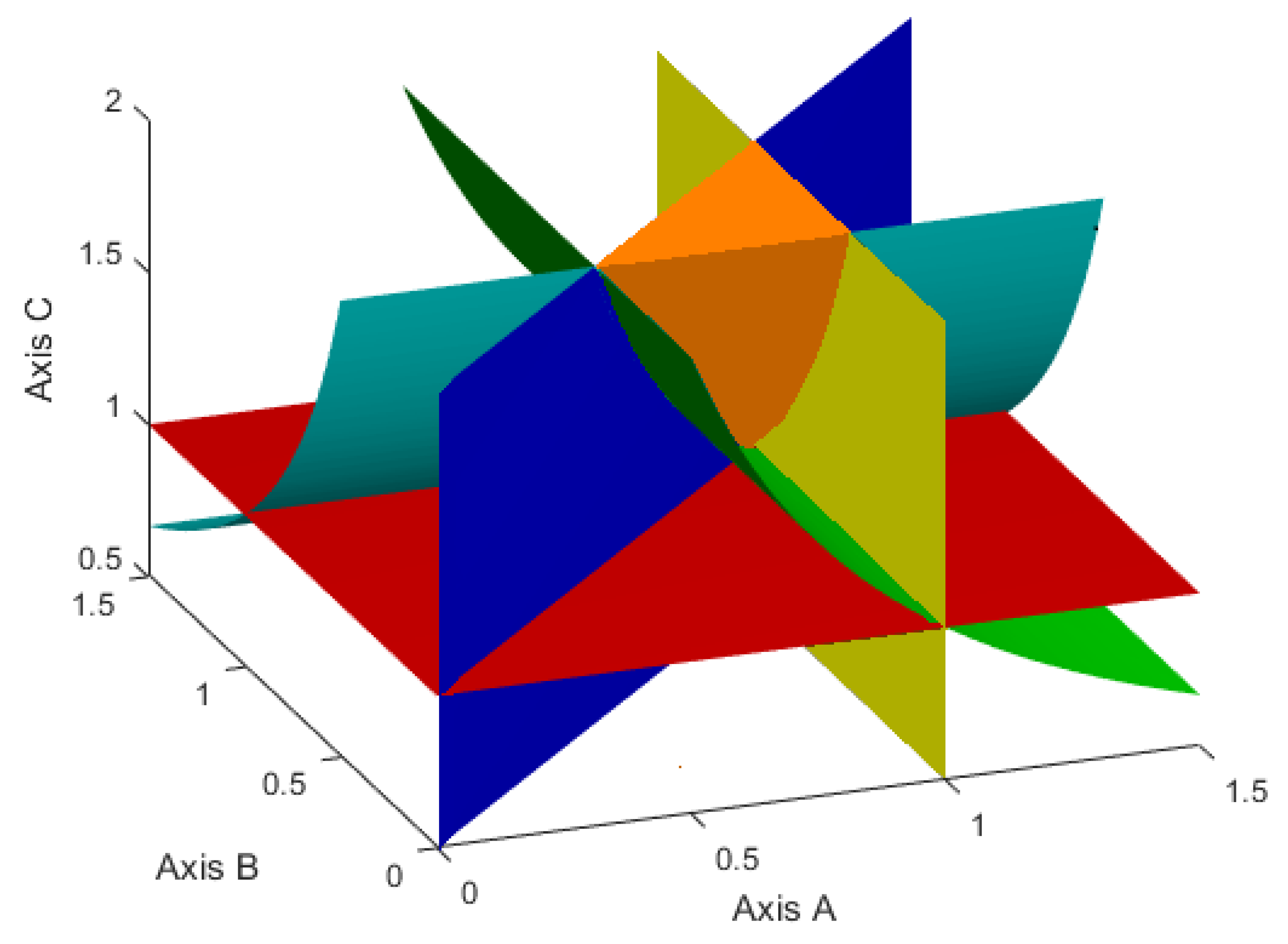
First, we will show that the set of parameters values given by inequalities (
3)–(
6) is not-empty. To do this, we will transform these inequalities by introducing new variables:
Due to them, the second inequality in (
3), as well as inequalities (
4) and (
5) are rewritten as
We note that the inequality (
6) is rewritten as
and therefore it can be considered separately, like the first inequality in (
3).
Then, in the positive octant of the coordinate system
, inequalities (
54) define the not-empty set, which is shown in
Figure 1.
Figure 2 demonstrates a similar set, but for the case when, instead of inequalities (
3), the inequalities (
24) hold. Such a set is given by the inequalities:
Therefore, further we will choose such values of the model parameters p, q, , , , , , , , so that they satisfy the following two cases.
Case 1. The inequalities (
3)–(
6), or, what is the same, the inequalities (
54) and (
55) are satisfied.
Case 2. The inequalities (
4)–(
6),(
24) or equivalent inequalities (
55) and (
56) are valid.
Now, we will demonstrate the results of a numerical solution of the minimization problem (
10). The values of the corresponding parameters were adopted from [
13,
14,
32] and chosen so as to show the numerical solutions for both of the above cases. Thus,
Figure 3,
Figure 4 and
Figure 5 presented below correspond to Case 1, and
Figure 6 and
Figure 7 relate to Case 2.
These numerical calculations were conducted using “BOCOP–2.2.0” [
33]. It is an optimal control interface, implemented in MATLAB, for solving optimal control problems with general path and boundary constraints and free or fixed final time. By a time discretization, such problems are approximated by finite-dimensional optimization problems, which are then solved by well-known software IPOPT, using sparse exact derivatives computed by ADOL-C. IPOPT is the open-source software package for large-scale nonlinear optimization. In the computations, we set the number of time steps to 3000 and the tolerance to
and use the sixth-order Lobatto III C discretization rule [
33]. In
Figure 3,
Figure 4,
Figure 5,
Figure 6 and
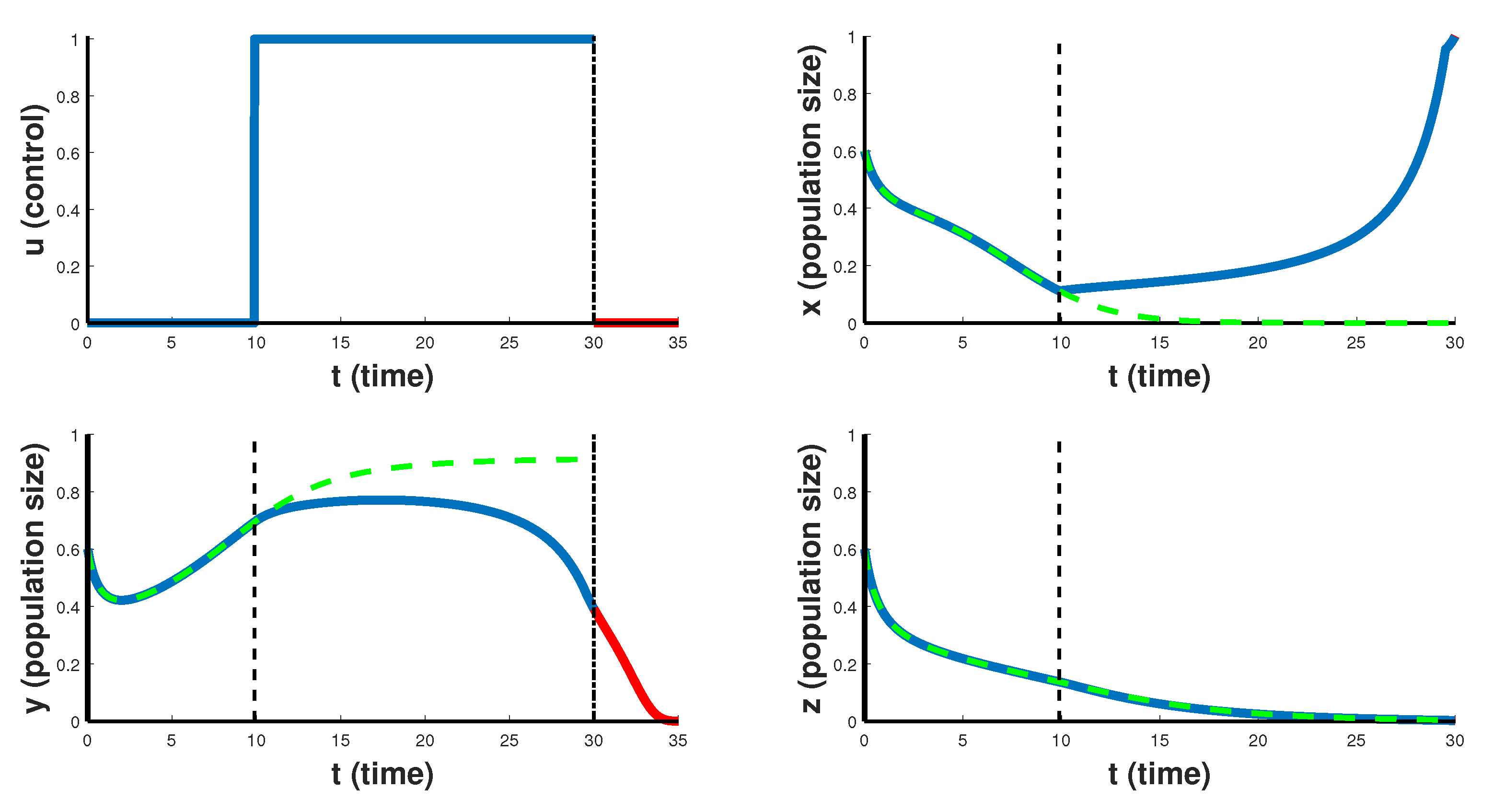
Figure 7 the blue lines represent the optimal solutions, whereas the green dashed lines represent the solutions in the absence of the control. The red lines show the continuations of the optimal solutions of the population of B-leukemic or cancer cells
for a longer time interval (in
Figure 3,
Figure 4 and
Figure 5 for
, and in
Figure 6 and
Figure 7 for
). The vertical dashed lines represent the switching moments. The end of the interval
is shown by the vertical dot-dashed lines.
In
Figure 3, the case of so-called emergency CAR T-cell therapy over 30 days treatment period is shown. Optimal control takes the maximum value
on the entire interval of the therapy, which helps to slow down the rate of proliferation of cancer cells, but still such therapy is not able to completely suppress the cancer. Note that after the end of the therapy period, cancer cells begin to grow rapidly in the first 5 days. This suggests that cancer is resistant to this scenario of CAR T-cell immunotherapy. Such emergency CAR T-cell therapy can only slow down the development of the cancer, and is a temporary solution for developing another course of treatment, but is not suitable for the patient’s recovery strategy.
The
Figure 4 and
Figure 5 reflect more optimistic therapy schedules. In
Figure 4 the case of CAR T-cell therapy delayed at the beginning is considered. For the first 10 days the optimal control
takes the minimum value 0, and then the therapy is carried out with maximum intensity
. In this case, CAR T-cells begin to grow and suppress the development of cancer. After the end of such therapy, cancer cells decrease to zero in the first 5 days. Such therapy leads to the destruction of cancer cells, which is an indicator of the higher efficiency of this course of therapy for the treatment of this type of cancer.
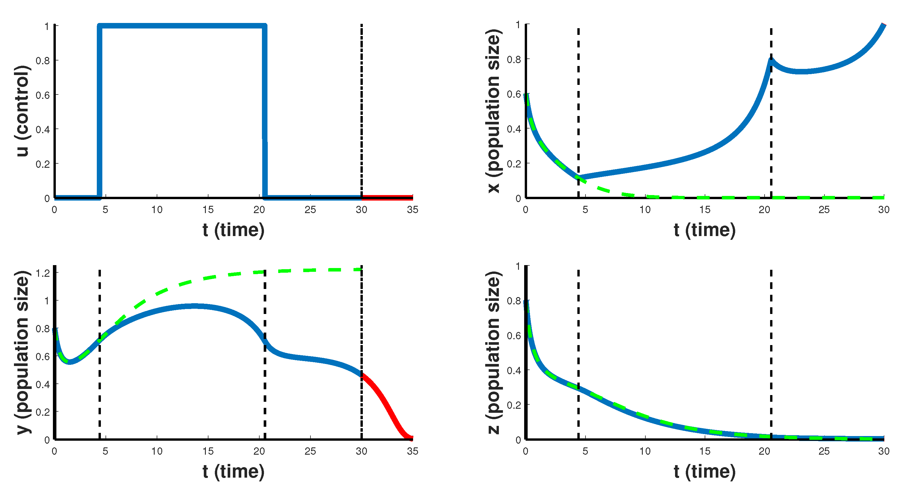
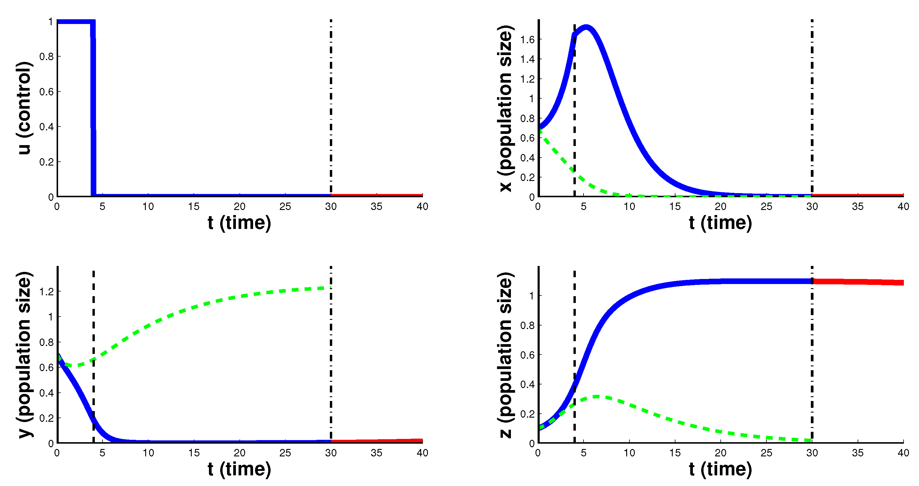
In
Figure 5 CAR T-cell therapy that is delayed at the beginning, of its maximal intensity in the middle and stopped at the end is shown. At the beginning of therapy, in the first 4 days, the injection of the chimeric cells is not performed, and then it is carried out with the maximum intensity
, which contributes to the reduction of cancer cells. On 21st day the therapy is again stopped. After the end of this therapy, cancer cells die out in the first 5 days. Here, as in the previous case, the treatment leads to the complete destruction of cancer cells.
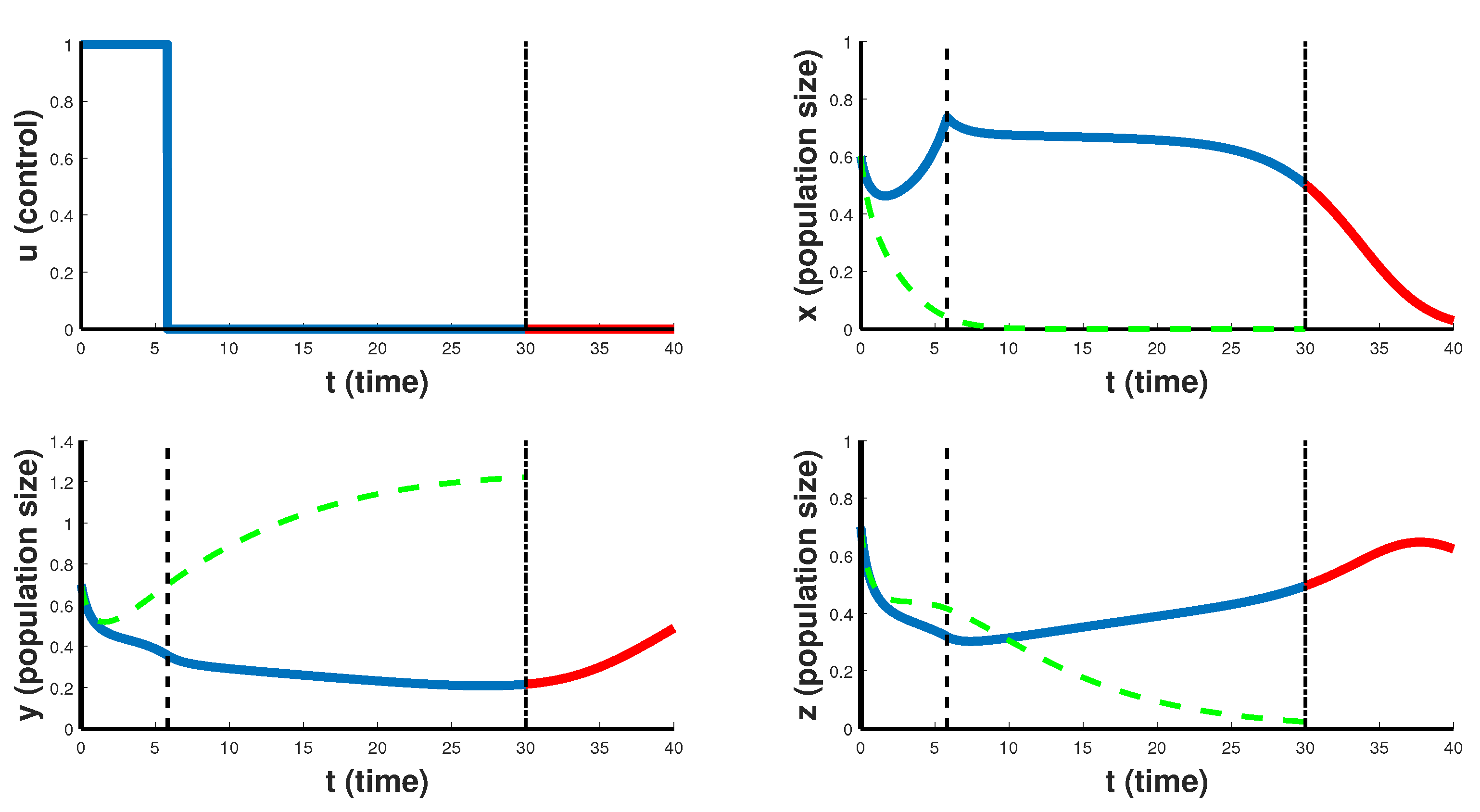
In
Figure 6 and
Figure 7 the case of CAR T-cell therapy stopped at the end is considered. For the first 4–6 days the optimal control
takes the maximum value
, and then the therapy is carried out with minimum intensity 0. In this case, CAR T-cells (chimeric cells) begin to grow and suppress the development of cancer. Although both figures are characterized by the same type of the optimal control, and both relate to Case 2, when
, they correspond to different situations. Thus,
Figure 6 refers to a situation when chimeric cells are as active in recognizing CD19 markers on healthy cells as on cancer cells, with
and
.
Figure 6 demonstrates a therapy that helps to slow down the rate of proliferation of cancer cells, but still cannot completely suppress the cancer. Note that after the end of the therapy period, for some time healthy cells still continue to grow, however, cancer cells begin to grow slowly in the first 10 days as well. This suggests that such treatment scenario can only slow down the development of the cancer, and is a temporary solution for developing another course of treatment, but is not suitable for the patient’s recovery strategy.
Figure 7 reflects the situation when
and so chimeric cells are more active in destroying cancer cells than on healthy cells. It is like a case of complete recovery from cancer.
Finally, we note that in all numerical calculations, the behavior of the cytokine population is the same regardless of its initial state . Due to the constant optimal control , taking its maximum value 1 over the entire treatment period, the size of this population quickly stabilizes to the value .
11. Conclusions
Recently, optimal control problems have become unfairly considered routine, since many authors use ready-made computer programs to solve them, without conducting any analytical investigation at all or reducing the latter to a minimum. It should be noted right away that in our work we use a Bolza-type objective function, the integral part of which does not contain square of the controls. Usually, a purely numerical solution of optimal control problems with such objective functions, without a preliminary analytical study of possible solutions, can be associated with certain computational difficulties. Anyway, it is difficult to look for a needle in a haystack. Therefore, we would like to emphasize the most important results obtained by us analytically.
In this paper, we stated and solved the optimal control problem with two bounded controls using the Pontryagin maximum principle. It should be noted that our analytical study of the controlled model allowed finding the type of optimal controls using the behavior of the switching functions. Thus, Theorem 1 states that the optimal control
is constant taking its maximum value over the entire time interval. This means that in order to prevent “a cytokine storm”, immunosuppressant drug must be taken at its maximal dosage over the entire treatment period. Further, Lemma 3 together with Theorem 2 state that depending on the model parameters and the values of the state variables at moment
T, the optimal control
can take either its maximum or minimum value. Our methods of analytical investigating are well described in
Section 5 (reducing the matrix of the linear non-autonomous system in a upper triangular form and then applying the Generalized Rolle’s Theorem to this system), in
Section 6, where we split the three-dimensional quadratic system into two simpler two-dimensional quadratic subsystems, in
Section 7, in which we provide an analysis of the quadratic subsystems, and finally, in
Section 8, where we estimate the number of zeros of the switching function
. Using this switching function properties, in
Section 9 we established that the optimal control
has at most two switchings that was also demonstrated by independent numerical results presented in
Section 10.
In this work, creating a controlled model of CAR T-cell immunotherapy, and solving the problem of an optimal control, we tried to explain some of the disadvantages of this procedure for treating leukemia and wished to find possible ways to increase its effectiveness. Within the framework of the proposed model and as a result of an analytical study of the switching function, five possible optimal treatment scenarios were obtained. The numerical results of the optimal solutions using BOCOP-2.2.0, as well as solutions without control, are shown in
Figure 3,
Figure 4,
Figure 5,
Figure 6 and
Figure 7. Note that the graphs of the optimal controls are in an excellent agreement with the corresponding Formulas (
52) and (
53), when fulfilled, they should be obtained. Thus, the optimal controls demonstrated in
Figure 3 (no switching) and
Figure 4 (one switching) end with their maximum value that is in an agreement with the Formula (
52) (
, and
, respectively), while for the graphs in
Figure 5 (two switchings),
Figure 6 (one switching) and
Figure 7 (also one switching), the Formula (
53) is satisfied (
,
, and
, respectively), and the optimal controls end with their minimum value.
Despite the fact that the optimal strategies shown in
Figure 4 and
Figure 5 lead to the destruction of cancer cells, also on these graphs, a sharp increase in chimeric leukocytes is noted, while the population of other cells is significantly reduced. Apparently, in an organism weakened by chemo- and radiotherapy, chimeric cells, instead of killing only cancer cells, begin to compete with both types of cells and continue to actively divide.
It should be noted that in all situations presented in
Figure 3,
Figure 4 and
Figure 5, the number of healthy lymphocytes is steadily decreasing over the given treatment period. It follows from the clinical experiences that the B-cell aplasia induced by CD19 CAR immunotherapy is rapidly reversed after CAR T-cells are ablated [
34]. In our model,
Figure 6 also shows the same behavior, and one can see that as soon as the therapy stops, an effect of B-cells aplasia is vanishing. (See the red piece of the
curve on the 5-day post treatment interval.) It is interesting that
Figure 7 demonstrates a situation where no aplasia occurs and shows that with the optimal control, healthy cells do not die at all.
In
Figure 3,
Figure 4 and
Figure 5, we indeed do not observe rapid increase in the healthy cells five days after the treatment period. How can you explain such a “strange” manifestation of the model? This could be explained by the fact that in the first three cases the body receives too many chimeric cells, which themselves proliferate in the process of interaction with cancer and healthy cells and therefore their influence remains after the end of treatment. Thus, they are not completely ablated, and their nonzero presence continues influencing the model dynamics.
After all, it was more logical to assume that in the first case (
Figure 3), cancer cells would certainly be destroyed more efficiently than in the other two cases. The reason is apparently in the properties of the model itself. It is known that in the treatment of blood cancer, chimeric leukocytes with the antigen to the CD19 marker, which is also found in healthy leukocytes, are used. In our model, this manifests itself in the third terms of the first and third equations of the system. According to this model, some of the chimeric cells spend their energy not on cancer cells, but on the destruction of healthy cells. Moreover, if maximum injections of chimeric cells are made, then this will immediately weaken healthy cells and will not launch a competitive mechanism between them and cancer cells, expressed by the last terms of the second and third equations of the model (
1).
Note that
Figure 3,
Figure 4 and
Figure 5 correspond to Case 1, when
and so chimeric cells very actively target healthy B-lymphocytes. Case 2, when
, presented by
Figure 6 and
Figure 7 seems to be more realistic. Thus, in
Figure 6, the concentration of healthy cells does not decrease in the course of treatment, even under initial conditions, when both cancerous and healthy cells have the same concentration. It is like a situation of modeling immunotherapy of leukemia in its severe stage. Moreover, it was found that if the initial concentration of cancer cells is significantly higher than the concentration of healthy cells, then the treatment according to
Figure 7 scenario becomes more effective.
Figure 7 demonstrates a case of recovery from leukemia, when cancer cells are completely destroyed, and healthy B-lymphocytes grow, reaching their equilibrium state.
It should be noted that for our numerical results, we chose such values of the model parameters in order to demonstrate all possible types of optimal control predicted analytically. It is possible that some of the Formulas (
52) or (
53) are not implemented at all in practice, but this was impossible to verify due to the unavailability of real data from clinical experiments.
Well, in principle, we need more specific chimeras that would recognize and kill only foreign cancer cells. For example, the CAR T-cell therapy can be specifically modified to stimulate the lymphocytes not too much, but not too weakly. In order not to stimulate the lymphocyte in the absence of a cancer cell, to better find rare markers on the surface of cancer cells. Mathematically such a case can be modeled by predator-prey model with further competition between cancer and healthy cells, mentioned in Introduction. This model would be implemented in our future studies.


