Does Informational Equivalence Preserve Strategic Behavior? Experimental Results on Trockel’s Model of Selten’s Chain Store Story

Abstract

The purpose of this study is to experimentally test Trockel’s game, which is a modelling of the classical Chain Store Game (CSG), and determine whether one of the two theories of Equality and Deterrence may better account for the observed behavior. The CSG is an example of a simple game in extensive form where the actual behavior of well-informed players cannot be expected to agree with the clear results of game theoretical reasoning. To explain the disagreement between the theory and the expected behavior, Trockel’s game is proposed as an alternative modelling of the scenario. The existence of more than one equilibrium in Trockel’s game opens a door for reputation building. This study is the first attempt to experimentally test this alternative game with the same purpose. According to my data, there is some evidence in favor of both Equality and Deterrence Hypotheses. However, since the strategies compatible with the Equality Hypothesis are played more frequently, I observe some patterns which share the same intuition with the Deterrence Hypothesis.

1. Introduction

Rational behavior refers to a decision-making process that is based on making choices that result in an optimal level of benefit. Thus, in the framework of rationality, we make choices for the sake of our long-term benefit, even if we pay the price by sacrificing some short-term gains. However, if we are expected to be ‘perfect rational’ (rational at each single decision), the time-feature evaporates from the decision process—as the chain store’s long-term payoff maximization is in conflict with this rationality concept in Selten’s Chain Store Story.

The CSG is based on the one-stage Chain Store Game (see Figure 1), which is a two-player extensive form game between a monopoly (a chain store) and a (potential) entrant. In the CSG, the one-stage Chain Store Game is played consecutively for 20 rounds with the same monopoly and each of 20 different (potential) entrants, who are observing all plays before it is their own turn to play. According to Selten’s story the potential entrant, who has enough capital, decides whether to enter the market or to stay out of the market completely. If this entrant decides to enter the market, then the monopoly employs one of two different monetary policies: Cooperative or Aggressive. A cooperative response yields considerably higher (duopoly) profits for both the monopoly and the entrant (both get 2 units of payoff, see Figure 1), as compared to an aggressive response (both get 0 unit of payoff, see Figure 1). In the latter case, however, the profit of the monopoly is much higher if the entrant does not enter the market (the monopoly gets 5 units of payoff, the entrant gets 1 unit of payoff, see Figure 1). The entrant prefers to stay out of the market and to use the capital in a different field instead, rather than to enter the market only to be met by an aggressive response. It is assumed that all the players wish to maximize their profits: for the monopoly, the total of the profits in 20-stage game and for an entrant, the profit of the one-stage game in which she decides. [1] discusses the CSG in two different ways: One is based on backward induction and the other on an intuitive deterrence argument. According to the Induction Hypothesis represented using the subgame perfect equilibrium concept, each entrant enters the market and then the monopoly always reacts with a cooperative monetary policy. According to the Deterrence Hypothesis, the monopoly should not behave in accordance with the Induction Hypothesis. By playing aggressively in the earlier stages, the monopoly may influence what future potential entrants think about its potential actions. If these beliefs turn into ‘aggressive monopoly beliefs’ early enough in the sequentially repeated game, the aggressive policy increases the monopoly’s profits in the long run. If that is the case, it is optimal for all potential entrants to stay out from the beginning. This way, the monopoly would earn higher profits in the long run than it would earn by following the Induction Hypothesis. The disagreement between these two hypotheses is called the ‘Chain Store Paradox’ in [1] and in the following related literature.

Ref. [2,3] remove the assumption of complete information and present versions of the CSG with incomplete information. In Figure 2, you may find the two-player stage games of these CSG versions. The uncertainty regarding the monopoly player created by the incomplete information in both of the versions may trigger a fear in ‘Aggressive’ monetary policy, and may therefore deter the entrants from entering the market. As long as uncertainty exists, ‘Aggressive’ play against early entrants may be rational because it creates a reputation that would deter future potential entrants. These modifications of Selten’s story were with largely the same approach via explicit introduction of incomplete information, but are obviously violating Selten’s informational assumption. Therefore, they could hardly be seen as solutions to the paradox, although they nevertheless have been perceived as such in the literature.

While the models of [2] and of [3] eliminate the complete information assumption, [4] keeps the complete information assumption but introduces an imperfect information game as an alternative model of Selten’s Chain Store Story. [4] shows that the paradox vanishes when using the ‘right’ richer model as the game theoretic presentation of Selten’s story, and one does not need to eliminate the rational player assumption in order to explain the ‘actual behavior’ in a game with rational players. Nor does one need the framework of perfect information. In other words, he shows that the paradox is not in Selten’s story, in Selten’s game. In Trockel’s game, Selten’s story is preserved; the only difference is in the order of moves made by the players (see Figure 3). Trockel’s game and Selten’s game are normal-form equivalent and informationally equivalent as defined by [5,6]1. Hence, the two-player stage games of [1,4] (Figure 1 and Figure 3) are equivalent in terms of decision-making.

The ‘Cooperative-In’ strategy set is the unique sequential (and perfect) equilibrium of Selten’s game. However, in Trockel’s game, together with ‘Cooperative-In’, the ‘Aggressive-Out’ strategy set is a sequential equilibrium and this equilibrium can be (re)enforced by building reputation. Reputation building is possible only if beliefs can be part of the model; thus, the existence of non-singleton information sets is the advantage of Trockel’s game as compared with Selten’s game. Furthermore, the existence of more than a single equilibrium allows for the chosen equilibrium strategy to be interpreted as a signal that reveals the kind of behavior that will consistently be displayed when the game is repeated. If that behavior can effectively be repeated in the next stages of the game, then reputation is built up via the entrants’ Bayesian updating of their beliefs. The other advantage of the game is the imperfect information. The type of reputation that might be built in Trockel’s game organizes the coordination of the choice in the respective equilibrium. Despite this additional structure Trockel’s game is offering, [4] models exactly the same scenario as Selten’s game—which is based on the Sure Thing Principle (see [7]), which guarantees the informational equivalence of Selten’s and Trockel’s games, is already embodied in von Neumann-Morgenstern utility functions assumed in standard Game Theory.

What Selten calls the Induction Hypothesis in the CSG is what I call Equality Hypothesis in Trockel’s game: the players play in such a way that the earnings of each can be equal. This hypothesis implies that there is no strategic connection between the stages, i.e., the decisions at stage games are perceived as mutually independent. In Trockel’s game, there is a situation in which every player can get the same amount of payoff—namely 2 * 20 = 40—by following the path of the ‘Cooperative-In’ sequential equilibrium. The outcome of this equilibrium is the desirable by all the entrants, since there are no situations in which they are better off. However, for the monopoly player, there is another and better alternative: the path of the ‘Aggressive-Out’ sequential equilibrium in which she might use building a reputation expressed by the updated beliefs of the entrants during the course of the play. The monopoly player should motivate some of the entrants to play ‘Out’ by constantly playing ‘Aggressive’ starting from the very beginning of the game. A weaker version of the behavioral pattern in the path of the ‘Aggressive-Out’ sequential equilibrium is what I call Deterrence Hypothesis in Trockel’s game. Like Selten explains, a monopoly player should decide on the basis of her intuition for how many of the last periods she wants to play ‘Cooperative’ (towards the end of the game, there is no concern about the reputation any more). She can have a higher payoff than 40, if she can convince sufficiently many early entrants that she insists on the payoff 5—the payoff of the monopoly player when an entrant plays ‘Out’.

Suppose that the monopoly player decided to play ‘Cooperative’ in the last 3 periods of the game. If the game is played in this way, she may get 17 * 5 + 2 * 3 = 91. If some more than expected of the entrants believe in the Equality Hypothesis, the monopoly player can still get more than 40. Imagine that not only the last 3 entrants, but also 10 of the other 17 entrants played ‘In’ and the other 7 played ‘Out’. In this case, the monopoly player will get 7 * 5 + 10 * 0 + 2 * 3 = 41, which is still better than 40. This means that it is sufficient to deter 7 entrants from playing ‘In’.

In the beginning of the game, if there are 2 to 3 entrants who decided ‘In’ when the monopoly player already decided to play ‘Aggressive’, this may lead the following entrants to fear losing and develop the tendency to the ‘Out’ decision. In the last phases of the game, even though the monopoly player is not planning to play ‘Aggressive’, this reputation effect can cause the 18th entrant’s ‘Out’ decision, maybe even the 19th entrant’s.

If the entrants believe that the monopoly player will follow the Deterrence Hypothesis, they also play accordingly. If the payoffs of the previously played entrants in all previous periods are 0, the next entrant should play ‘Out’ unless she thinks that the game is sufficiently close to the end.

The purpose of this paper is to test Trockel’s game and determine which of the two hypotheses better accounts for the outcome: the Equality Hypothesis or the Deterrence Hypothesis. Moreover, I aim to observe whether it is possible to deter the potential entrants in Trockel’s game by building reputation. Understanding what affects the behavior of the players, how the behavior of the players changes, and whether the strategic behavior is preserved as a result of the equivalent information with the CSG are the main motivations of the study. Put differently, my goal is to study whether equivalence in information preserves strategic behavior. To the best of my knowledge, this study is the second experiment that clings to this scenario, and the first attempt in the literature that experimentally tests Trockel’s game with the same purpose of understanding whether entry deterrence is possible. Selten’s scenario had been tested in the laboratory for the first time and 20 entrants—as Selten suggests—are used for the first time. The introduction of investment (representing the capital in the story) in the design constitutes the major difference from the main design in [8].

My data cannot be explained solely by the Equality or the Deterrence Hypothesis, as either of these hypotheses is supported by some evidence. Although the strategies compatible with the Equality Hypothesis, ‘Cooperative’ and ‘In’ were played more frequently, I observe some similar patterns which share the same intuition with the Deterrence Hypothesis. More specifically, the history of the decisions, the round number (or, the number of the rounds left to play), previous earnings and the type of last decision by the opponent have an effect on the decisions of the entrants; and for the monopoly player, the type of the responses obtained after ‘Aggressive’ play matters as well as the round number (or, the number of the rounds left to play).

Experimental Literature

One of the referees for this article suggested in a footnote to hint to the political application of the analysis of the Chain Store problem to federal systems. In fact, when it comes to the importance of experimental results I think it is worth more than just a footnote. In particular, he wrote:

“In the U.S., for example, there are two main, state-sponsored parties. In many states, the Republicans (“Red State”) or Democrats (“Blue State”) are dominant. Sometimes a third party, of various sorts, may try to enter. But this entry usually takes place in one state, or at most a few states. The dominant party in that state is likely to spend more money on the campaigns (Governor, Senate, US House, etc.) to prevent the aspiring entrant from gaining a foothold. Or, do they? It’s expensive, and doesn’t really deter third parties, who don’t expect to win anyway. Aaron King works some of this out in his book (pp. 35–40).”

Also, in the law of economics literature, a similar problem has been an important issue under the name of predatory pricing. It is discussed in detail in Section 8 of Chapter 10: The Antitrust Laws in the famous book [9] by Richard Posner. The question whether predatory pricing could be punished by law when it could not be expected to be used by rational firms gave rise to the entrance of predatory pricing into the game theoretic literature. Without support from experimental evidence, the influence of game theoretical analysis on the clarification of this issue would remain quite limited.

Ref. [10] discusses the CSG from the perspective of Political Science. According to their study, politics is inherently strategic, and bluffing is the basic ingredient of this strategy. The CSG and its multiple versions are used by [10] to explain the role of reputation based on bluffing and commitment in international politics. Both bluffing and commitment are defined as tools to manipulate the expectation(s) of the opponent and, consequently, lead to a change in the opponent’s behavior. They explain the modelling of [2,3] with bluffing, and the modelling of [4] with commitment (threat). They support the plausibility of benefit via reputation by real-life examples on developing and maintaining leadership.

The experiment literature includes several studies on the CSG, entry deterrence and predatory pricing: see e.g., [8,11,12,13], where [11] is one of the first attempts in the literature focusing experimentally on reputation and price predation. They use their borrower-lender game that has strategic aspects in common with the CSG, and their result shows strong reputation effects and the rationality of price predation.

The other referee wrote: “Trockel’s game does not seem conceptually very different from a hawk–dove game. This similarity should be made explicit, and the experimental literature on hawk–dove should be mentioned.” There are experimental studies focusing on reputation, deterrence, fairness or equity in the hawk–dove game: see for example [14,15].

However, the equivalent CSG modellings of Selten and of Trockel are neither informationally nor normal-form equivalent to the hawk–dove game. It is easy to write down a bi-matrix for the hawk–dove game, that, other than the Chain Store game, belongs to the class of so-called anti-coordination games and like the CSG has exactly the numbers 5, 2, 1 and 0 as occurring payoffs. It has two equilibrium payoff vectors (1,5) and (5,1) both Pareto optimal, while the CSG has two Pareto efficient equilibria with payoff vectors (5,1) and (2,2), where the first one’s payoffs are independent of any (anti-) coordination. I therefore abstain from delving into the experimental literature of the hawk–dove game.

Ref. [12] test the asymmetric information version in [2] with 7 short-run players. In a session, 3 monopoly players and 4 entrants participate. One monopoly player faces 4 entrants, then the other 2 monopoly players face the entrants, and 4 entrants face the first monopoly player again by shuffling the order of the entrants. In 4-periods phases, usually ‘Aggressive’ play was preferred. Thus, they find support for the existence of a sequential deterrence equilibrium, even with a ‘weak’ monopoly player. Ref. [8] is the first in the literature to attempt to study the original CSG by employing experimental methods. Their study contains two treatments with 10 monopoly players and 15 entrants, respectively. Although the statistically significant support for the Deterrence Hypothesis amplifies as the number of the entrants increases, the support for entry deterrence with ‘Aggressive’ play is not observed. The authors concluded that 15 entrants were not adequate to make the deterrence argument effective and pointed out the necessity of a study with at least 20 entrants. Ref. [8,16] offer suggestions for future studies of the CSG. Some of them call for an increase in the number of entrants (20 or more), another design of a laboratory experiment, and the use of Trockel’s game. All these suggestions have been dealt with in the present study.

Ref. [13] presents a new version of the CSG with an additional move for the entrants in which they have the chance to either stay in the market or exit the market after the monopoly player’s ‘Aggressive’ play. Unlike the other experimental studies, the participants may communicate with each other before submitting their decisions. They were informed about the following concepts: backward induction, the Nash equilibrium, and the Prisoner’s Dilemma. Ref. [13] reports that none of the monopoly-type participants responded aggressively on a consistent basis.

All experimental studies described above are conducted as paper-and-pencil experiments. Unlike these, a laboratory experiment is conducted in this study. The design is closer to the design of Experiment 3 in [8], but Trockel’s game is used instead of Selten’s game. The other difference from the design of [8] is in the use of the investment. Investment represents the necessary capital to establish a store for an entrant and the value of a store for a monopoly. Hence, a design without investment cannot properly motivate the participants as described in the scenario. Even if there is no data to examine the difference between the design with and the design without the investment, the results are expected to be different in each, based on the endowment effect (or loss aversion) in the literature [17].

The starting point of this study was the question of whether equivalence of information in two different games preserves strategic behavior. The conjecture was that the answer is negative by identifying the question with the framing effect [18]; i.e., the different results can be expected from the experiments simulating the CSG and Trockel’s game. More specifically, ref. [4] changes the order of play in each stage game of the original game in an informationally equivalent way, and this change can be interpreted as a framing effect. Since I did not run any experiment based on Selten’s original game and I cannot directly compare my results with the results of [8], this statement is not more than an anticipation that is not properly tested in this study.

Although Game Theory neglects the difference in the information flow in the CSG and Trockel’s game, there are studies that negatively answer questions similar to those I asked to myself. Ref. [19] conducts three experiments with strategically equivalent games in extensive form, and the results show that there is a significant difference in how the games are played. Ref. [20] provides support for the importance of the order of play. According to their results, the advantage of a player in a game can be destroyed by changing the order of play. Hence, if it is assumed that the entrants have an advantage in the CSG, this can be damaged by Trockel’s game.

2. Experimental Design

A laboratory experiment was designed to simulate Trockel’s game. The design is almost the same as the last version of the design in [8]. The z-tree program by [21] was used to implement a laboratory experiment.

2.1. Subjects

In Spring 2017, the undergraduate students from several faculties of Istanbul Bilgi University (IBU) and Middle East Technical University (METU) were contacted and, 576 of them volunteered to participate. The students were recruited by the online system ORSEE [22].

The experiment was conducted in two laboratories: BELIS (Bilgi Economics Lab Istanbul) and BAEL (Behavioral and Experimental Lab, METU). In each university 12 sessions were conducted, for 24 sessions in total. Each session was completed in approximately 75 minutes.

For each session, 24 participants were invited. Written instructions were placed in every computer cubicle, so that the participants could follow them when they were aloud.

2.2. Types

In the beginning of the experiment, the 24 participants were assigned randomly to two roles: 4 of them were assigned to type M (representing the monopoly player in the scenario) and 20 of them were assigned to type E (representing the entrants in the scenario). To distinguish between the players, a positive number was assigned to each player: numbers between 1–4 for type M players; and numbers between 1–20 for type E players. Hence, the players in each session were numbered by M1, M2, M3, M4 and E1, E2,…, E20.

2.3. In-Experiment Matchings

There were 20 rounds in the experiment. Throughout the rounds, all the type M participants were active and matched with each type E participant, but in a different order. This implies that each type E participant played once with each type M participant, in total 4 times. Therefore, each type E participant was active in 4 out of 20 rounds and waited in the remaining 16 rounds for the next round in which she will be active or the termination of the experiment.

Due to the active and inactive rounds of type E participants, it was necessary to control the matchings of the two types of participants to observe their behavior in each phase of the rounds, to equalize their level of getting experienced in the experiment, and also to avoid the situations in which a type E participant would play successively. For those reasons, 20 rounds were divided into 4 sections, each containing 5 rounds. Each type E participant played once in a randomly chosen round of each section and in each section she matched with a different type M participant. As soon as the experiment started, the program announced to all the type E participants the rounds in which they would be active, and with whom they would be matched in these rounds.

2.4. Periods

Each session included 20 rounds. Each round contained 4 independent one stages of Trockel’s game (see Figure 4) and each session is made up of 4 twenty-round Trockel’s games in which all type M participants played against all type E participants, but in a different order. In other words, every type M participant and her type E opponent (determined randomly in the beginning of the experiment) played one stage of Trockel’s game in each round. Throughout the rounds, each type M participant played with a different type E participant and, consequently, a type M participant played once with each of the 20 type E participants.

The type M participants were not informed about the matches of the other type M participants, so the experiment was mutually independent for type M participants.

Each of the activated participants in every round was given 1 point. This is used to plug the investment instrument of the scenario into the experiment.

In each round, type M participants moved first by choosing one of the actions: ‘Agg’ or ‘Coop’. Importantly, the decisions of type M participants were announced to none of type E participants. After the type M participant made a decision, it was time for the type E participants activated in this round to make a decision. The type E participants chose one of the actions: ‘In’ or ‘Out’.

The payoffs were the same as used in the Trockel’s game, as depicted in Figure 4. After the type E participants submitted their decisions, each of the active participants was informed about her own payoff as well as the payoff of the opponent. After the announcement of the payoffs, the experiment continued with the next round in which type M participants were matched with four new type E participants. After the completion of the 20th round, the experiment ended.

2.5. History Tables

At the end of each round, the payoffs were stored in the history tables which were displayed on individual screens. By the help of these history tables, the participants could follow the related previous rounds at the rate allowed by their types.

The history table for type M participants portrayed information about their own decisions and payoffs for all previous rounds as well as the decisions of their opponents in all the previous rounds. In

Table 1. An Example of a History Table of a Monopoly Player.

Round	My Decision	My Opponent’s Decision	My Points
1	Coop	Out	5
2	Agg	In	0
3	?	?	?

, you may see an example of the history table for a type M participant while the round 3 is ongoing.

The history table for active type E participants provided information about the payoffs (not decisions) of the opposing type M participant as well as the decisions and payoffs of the previously active type E participants, who already had played against this type M participant in previous rounds. In

Table 2. An Example of a History Table of an Entrant.

Round	The Decision of Type E who was Active in that Round	The Points of Type E who was Active in that Round	The Points of the Opponent
1	Out	1	5
2	In	0	0
3	?	?	?

, you may find an example of the history table for a type E participant while the round 3 is ongoing.

A waiting type E participant’s table contains the information about the matches of the type M participant with whom this type E participant was scheduled to match next; i.e., the table is the same as that of the active type E participant who was matched with that type M participant.

2.6. Treatments

There were two treatments:

• First treatment T1: Trockel’s game is used with the original payoffs.
• Second treatment T2: It differs from T1 in the payoff of the monopoly when the outcome is ‘Aggressive-Out’. In T2, the payoff increased from 5 to 10 when the entrant chose ‘Out’, to enhance the appeal of ‘Aggressive’ play.

2.7. Questionnaire and the Payment

A questionnaire that helps to understand the reasons for the participants’ behavior during the experiment was started after the completion of the rounds. This questionnaire was the version of the one in [16]. The questions were adapted to the modification of Trockel’s game, but their aims were preserved (see Appendix A).

After the questionnaire, the participants were paid their earnings and the session was completed. The total amount of what a type M participant earned in each round was paid in Turkish Lira (TL) and the total amount of what a type E participant earned in each round in which she was activated was first multiplied by 5 and then paid in TL.

3. Results

From each of the two universities, 288 undergraduate students took part in the sessions. Hence, 480 entrant data points and 96 monopoly player data points were collected, which are given in

Table 3. Pooled Data.

Round	Agg. Frequency	P(Agg)	In Frequency	P(In)
1	17	18%	65	68%
2	35	36%	62	65%
3	22	23%	64	67%
4	33	34%	66	69%
5	32	33%	68	71%
6	32	33%	72	75%
7	34	35%	69	72%
8	25	26%	78	81%
9	27	28%	74	77%
10	21	22%	84	88%
11	32	33%	77	80%
12	31	32%	70	73%
13	32	33%	81	84%
14	34	35%	74	77%
15	25	26%	82	85%
16	28	29%	70	73%
17	26	27%	79	82%
18	22	23%	73	76%
19	20	21%	77	80%
20	16	17%	82	85%
Total	544		1467
Mean	27.20	0.29	73.35	0.76
Std. Dev.	5.98	0.07	6.55	0.07

.

The mean payment of monopoly players was 46.86 TL (IBU 43.71, METU 49.96) in T1 and 71.5 TL (IBU 69.59, METU 73.42) in T2. The mean payment of entrants was 28.17 TL (IBU 28.71, METU 27.62) in T1 and 27.06 TL (IBU 26.63, METU 27.5) in T2. The lowest payoff earned by the METU monopoly players is 41 TL, exceeding the 40 TL that might have been earned by adhering to ‘Cooperative-In’. Except for two of the IBU monopoly players (although each played ‘Aggressive’ at least 12 times), all participants gained more than 40 TL. The mean entrant payoff is approximately 12 TL, which is also less than the amount possible by the ‘Cooperative-In’ sequential equilibrium.

In Table 3, the Agg. Frequency column shows the aggressive frequencies by round number. The monopoly players played ‘Aggressive’ on 29% of 96*20 rounds. One cannot say that the trend of the aggressive frequencies is upward or downward, but it is certain that the frequencies in the last 5 rounds decrease by the round number (see Figure 5).

In Table 3, the In Frequency column shows the entry frequencies by entrance order/round number. Altogether, the entrants played ‘In’ on 76% of 96*20 rounds. One can easily see that In Frequency varies as the round number increases (see Figure 6). Moreover, with a few deviations, it increases monotonically.

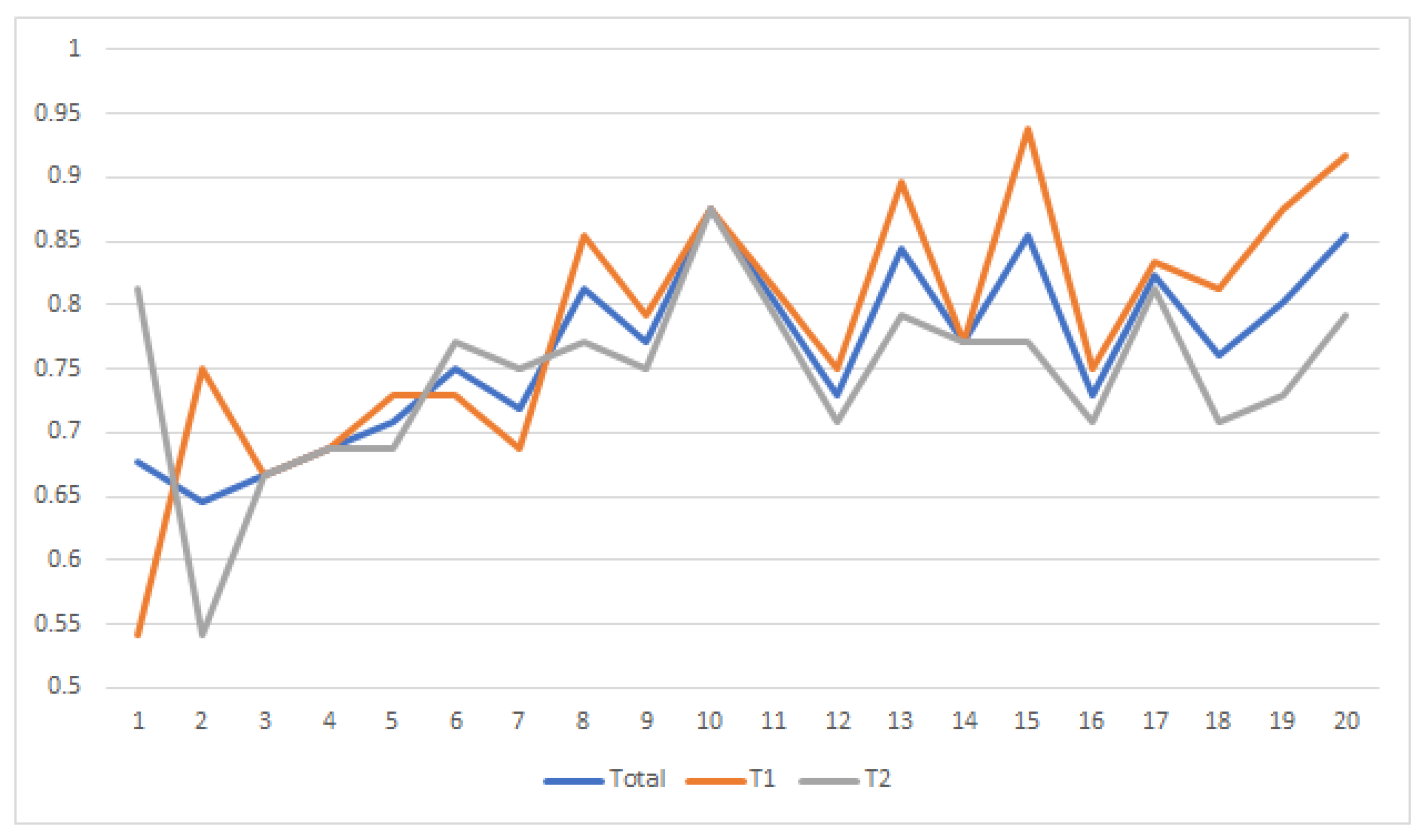
8 monopoly players (8%) always played ‘Cooperative’, while none of the monopoly players always played ‘Aggressive’ and only 3 monopoly players (4%) played ‘Aggressive’ at least 17 times. The ones who played a 50-50 mix of ‘Cooperative’ and ‘Aggressive’ are 5 out of 96 monopoly players (5%) and those who played ‘Aggressive’ at least 10 times are 17 out of 96 monopoly players (18%). Hence, approximately 86% of the monopoly players played a different mixed strategy than 50-50. A one-sided t-test rejects the hypothesis that subjects mix ‘Cooperative’ and ‘Aggressive’ with equal probabilities: ‘Cooperative’ is played significantly more frequently than ‘Aggressive’ (p-value $3.3067\times {10}^{-15}$). Moreover, I also focused on the post-behavior of the monopoly players who reached a 40 payoff within the first 17 rounds. After gaining a 40 payoff, the monopoly players played ‘Aggressive’ less frequently than how they played before the 40 payoff (p-value 0.037).

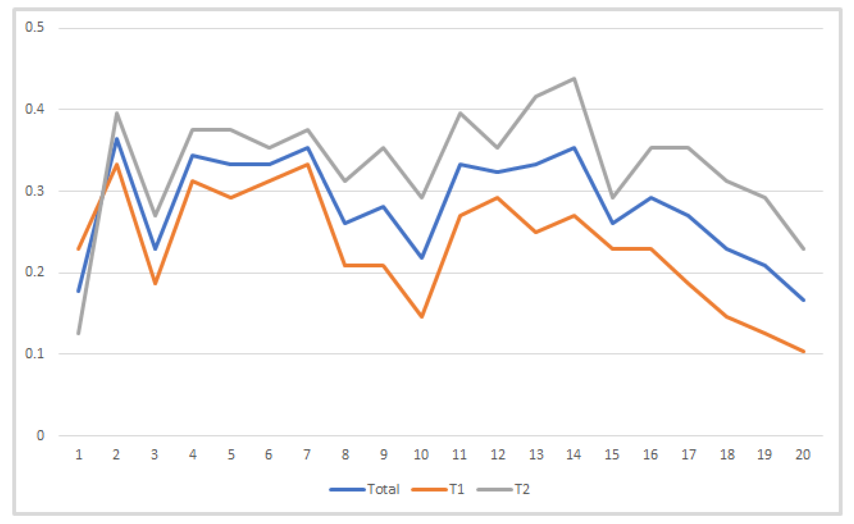
The number of the entrants who always played ‘In’ is 194 out of 480 entrants (40%), while only 12 entrants (2.5%) always played ‘Out’, and 77 entrants (16%) played a 50-50 mix of ‘In’ and ‘Out’. Among these 77 entrants, 46 entrants (9.5%) chose ‘Out’ as the first two decisions. Hence, approximately 41.5% of the entrants played a different mixed strategy than 50-50. A one-sided t-test rejects the hypothesis that subjects mix ‘In’ and ‘Out’ with equal probabilities: ‘In’ is played significantly more frequently than ‘Out’ (p-value $9.17107\times {10}^{-80}$).

To see some patterns that the data might have, we turn to the analysis of the Deterrence Hypothesis. The essence of the Deterrence Hypothesis states that the behavior of the entrants is not invariant to their order of play. To confirm whether this conjecture is valid for the data, all the decisions of each round were listed in such a way that the ‘Aggressive’ (‘Cooperative’) decision is coded as 1 (0), so that 20 different lists were such constructed. The Kruskal-Wallis H (one-way) test was conducted on these lists to determine whether there are any statistically significant differences between their means. The results show that the behavior of the monopoly players is not invariant across rounds (p-value 0.0147), nor is the behavior of the entrants (p-value 0.0004). Thus, the behavior of the monopoly players is not the same in all rounds, nor is the behavior of the entrants the same across all 4 rounds of play. It is important to understand whether the variability in the decisions of both monopoly players and entrants is due to the round number, or to the change in the information related to the round number might be the basis of the variability. Later, in Section 3.1, I employ logistic regression analyses to answer this question.

The proportion of ‘Aggressive’ play from round 1 to round 15 by the monopoly players significantly exceeds the same proportion in rounds 16 to 20 (one-sided t-test, p-value 0.0022) (see Figure 5). Please note that this difference may also be attributed to end effect [23]. Figure 5 leads us to consider the difference between the proportion of ‘Aggressive’ play by the monopoly players from round 1 to round 5 and the corresponding proportion in the last 5 rounds. The mentioned proportion in the first 5 rounds is greater than the one in last 5 rounds, and this difference is significant (one-sided t-test, p-value 0.004). Additionally, there is a significant difference between the proportion of ‘Aggressive’ play from rounds 6 to 15 and the corresponding proportion in the last 5 rounds (one-sided t-test, p-value 0.00093): The proportion between rounds 6 and 15 is greater. Finally, the difference between the proportion of ‘Aggressive’ play from rounds 1 to 5 and the corresponding proportion between rounds 6 to 15 is not a significant difference. Hence, the mean frequency of ‘Aggressive’ play in the first 15 rounds statistically exceeds the mean frequency of ‘Aggressive’ play in the last 5 rounds.

It is also important to determine whether the behavior of the entrants varies over sections. For this purpose, for each section I listed the numbers of ‘In’ responses to each monopoly player during the section. The Kruskal-Wallis H (one-way) test was conducted on these four lists to determine whether there are statistically significant differences between their means. The null hypothesis of equal means across all 4 sections is soundly rejected (p-value $4.08\times {10}^{-05}$). Hence, the choices of the entrants are not the same across the four sections.

The present experiment includes two treatments that differ from each other in their payoff (either 5 or 10) to the monopoly player when the outcome is ‘Aggressive-Out’. An increase in the proportion of ‘Aggressive’ choices is expected with the increase in payoff from 5 to 10, and the proportion of ‘In’ play is expected to decrease. A Kruskal-Wallis H (one-way) test was conducted on the number of ‘Aggressive’ play and separately on the number of ‘In’ play to test these two hypotheses about the effect of change in payoff. The results of the test show that monopoly players do not play the same way in the two treatments (p-value 0.0001). As expected, they support an increase in the proportion of ‘Aggressive’ play for the monopoly player. However, the expected statistically significant decrease in the ‘In’ play of the entrants is not supported (p-value 0.28). As a result, in ‘Aggressive-Out’ games, the choice of the entrants is not affected by the payoff of the monopoly player, while the choice of the monopolies is affected.

3.1. Logistic Regression Analysis

In this section, I present the results of logistics regression analyses conducted on the probability of an ‘In’ decision of the entrants or of an ‘Aggressive’ decision of the monopoly players. In the analyses, I use the fixed-effects and the random-effects model, which differ in the approach on the effects of the time-invariant variables. In fixed-effects model, the effects of the time-invariant variables are assumed to be time-invariant (so they are omitted), while it does not hold for the random-effects model. For example, one can suppose that the effect of the university in which a student studies does not vary through the rounds (fixed effect), but on the other hand, since a woman is expected to be more risk-averse than a man, she may change her behavior within the stages of an experiment under the pressure of losing(random effect).

Below, first you may find the results of two different logistics regression analyses of the entrants with each of two models, and later, the results of two different logistics regression analyses of the monopoly players with each of two models. In each table below, the first row of an independent variable presents the results of the fixed-effects model; and its second row belongs to the analysis with the random-effects model.

The panel data is obtained by combining the observations collected from IBU and METU participants, and then panel logistic regression analyses were conducted to estimate the probability of an entrant choosing ‘In’. The binary dependent variable is 1 if the decision is ‘In’, and 0 if it is ‘Out’. The independent variables are as followings: Agg is the number of ‘Aggressive’ decisions of the current monopoly player in the previous rounds, Uncertain is the number of Uncertain decisions of the current monopoly player in the previous rounds2, Round represents the number of the playing round, PRP is the payoff gained from the last play, LRA is a binary variable indicating if the last decision of the current monopoly player is ‘Aggressive’ or not, LRU is a binary variable indicating if the last decision of the current monopoly player is ‘Uncertain’ or not, Order represents the total number of consecutive decisions of the entrants (i.e., 1st or 2nd decision), Uni indicates at which university the entrant studies (at METU or not), Faculty represents in which faculty the entrant studies (Arts and Sciences/Social Sciences, Engineering, Architecture, Economics and Administrative Sciences/Business, Communication, Law or Education), Gender represents whether the entrant is female or not, Game Theory indicates if the entrant took a course on Game Theory or not, and ID is the identity number of the student.

Table 4. Entrants-Panel Logistic Regression 1.

Action	Odd Ratio	Std.Err.	z	$\mathit{P}>\mid \mathit{z}\mid$	$\%95$ Conf. Interval
Agg	0.7868992	0.0330637	−5.70	0.000 ***	0.7246922	0.8544459
	0.7723197	0.0306647	−6.51	0.000 ***	0.714497	0.8348219
Uncertain	0.813862	0.0371601	−4.51	0.000 ***	0.7441934	0.8900528
	0.8244335	0.0355853	−4.47	0.000 ***	0.7575564	0.8972145
Round	1.157306	0.0247897	6.82	0.000 ***	1.109725	1.206927
	1.142695	0.022985	6.63	0.000 ***	1.098522	1.188645
PRP	1.223414	0.1132568	2.18	0.029 *	1.020409	1.466807
	1.423831	0.1165063	4.32	0.000 ***	1.212853	1.67151
Uni	1	(omitted)
	0.7344255	0.1119438	−2.03	0.043 *	0.5447591	0.9901271
Faculty	1	(omitted)
	0.9905217	0.0520703	−0.18	0.856	0.8935472	1.098021
Gender	1	(omitted)
	0.6538374	0.0976447	−2.85	0.004 ***	0.4879222	0.8761711
Game Theory	1	(omitted)
	1.384987	0.213229	2.12	0.034 *	1.024229	1.872814
Constant
	2.597589	0.6460961	3.84	0.000	1.595335	4.229501

Std.Err. = Standard Error; Conf. = Confidence; *: P < 0.05; ***: P < 0.01.

presents the result of logistic regression analysis with the fixed-effect model on the panel data gathered from the entrants. The model is meaningful (p-value < 0.01) and all variables contribute significantly to the probability of an ‘In’ decision. While Round and PRP have positive effects on the probability, the other variables have a negative effect.

The odd ratio of the variable Agg is approximately 0.79 as shown in Table 4. If Agg increases by 1 unit, then the odd ratio of an ‘In’ decision decreases by a factor of 21%. That means that an increase in Agg observations results in a decrease in the probability of an ‘In’ decision. Hence, it is evident that the entrants are affected by the decisions of the monopoly players and, accordingly, they decide to either enter or stay out of the market. Furthermore, the entrants are affected by the undetermined decisions of the monopoly players in the same manner as they are affected by the ‘Aggressive’ decisions since the odd ratio of the variable Uncertain is approximately 0.81. If Uncertain increases by 1 unit, then the odd ratio of an ‘In’ decision decreases approximately by a factor of 19%. In other words, an increase in Uncertain observations decreases the probability of an ‘In’ decision. The entrants are reinforced to enter the market when they observe more ‘Cooperative’ decisions; alternatively, they decide not to enter the market (i.e., are deterred from entering the market) when they observe more ‘Aggressive’ play.

The variable Round is one of the positive-effect variables with the odd ratio approximately 1.16. Whenever Round increases by 1 unit, the odd ratio of the ‘In’ decision increases approximately by a factor of 16%. The probability of an ‘In’ decision increases if Round increases. One can infer that this result is evidence that entrants were sensitive to the round number or the information changing as a result of the increase in the round number.

The other positive-effect-predictor is PRP: the odd ratio is approximately 1.22. The probability of an ‘In’ decision is higher if PRP is high. This variable and its effect can be interpreted as a risk attitude, since entering the market is simultaneously the decision of risking the investment. If there is something in the ‘pocket’, one may assume risk more often; i.e., an entrant may have an incentive to choose ‘In’ again if she has already earned 1 more point with ‘In’.

Another logistics regression analysis was conducted with the random-effects model by using the same predictor variables. In Table 4, you may also find the results of it. All the predictor variables of the fixed-effects model to estimate the probability of ‘Aggressive’ decision are also predictor variables of the random-effects model. Among the time-invariant variables, Uni, Gender have a negative effect on the probability, while Game Theory has positive effect.

In Table 4, the odd ratio of the variable Uni is approximately 0.73, i.e., the probability of an METU entrant to have an ‘In’ decision is less than the probability of an IBU entrant. As stated in Table 4, the odd ratio of the variable Gender is approximately 0.65. This implies that a female entrant’s probability of an ‘In’ decision is smaller than a male entrant. This observation can be explained by the difference in the risk attitudes between the genders.

Some of the participants were the students who already took some courses on Game Theory. According to the odd ratio greater than 1, the probability of an ‘In’ decision is higher if an entrant had already learnt some basic concepts of Game Theory.

In

Table 5. Entrants-Panel Logistic Regression 2.

Action	Odd Ratio	Std.Err.	z	$\mathit{P}>\mid \mathit{z}\mid$	$\%95$ Conf. Interval
PRP	1.368848	0.1043251	4.12	0.000 ***	1.178914	1.589383
	1.517539	0.1053483	6.01	0.000 ***	1.324491	1.738724
LRA	0.4019908	0.0698842	−5.24	0.000 ***	0.2859162	0.5651888
	0.4431788	0.0690054	−5.23	0.000 ***	0.3266194	0.6013341
LRU	0.5323112	0.0885989	−3.79	0.000 ***	0.3841404	0.7376346
	0.4844501	0.0727617	−4.83	0.000 ***	0.3609136	0.6502717
Uni	1	(omitted)
	0.7629754	0.1124712	−1.84	0.066	0.5715231	1.018561
Faculty	1	(omitted)
	0.9960464	0.0511204	−0.08	0.938	0.9007268	1.101453
Gender	1	(omitted)
	0.6699686	0.097497	−2.75	0.006 ***	0.5037135	0.8910977
Game Theory	1	(omitted)
	1.361758	0.2046238	2.05	0.04 *	1.014365	1.828122
Constant
	4.732442	1.144424	6.43	0.000	2.946071	7.601992

Std.Err. = Standard Error; Conf. = Confidence; *: P < 0.05; ***: P < 0.01.

, the result of the second logistic regression analysis on the entrants’ panel data with fixed-effects model is presented. The model is meaningful (p-value < 0.01). The variables PRP, LRA and LRU contribute significantly to the probability of an ‘In’ decision. While PRP has positive effects on the probability, LRA and LRU have a negative effect.

The odd ratio of the variable PRP is approximately 1.37 as shown in Table 5. This means that the probability of an ‘In’ decision is higher if PRP is high. In other words, an entrant may have an incentive to choose ‘In’ again if she has already earned 1 more point with ‘In’.

The odd ratio of the variable LRA is approximately 0.40, i.e., if LRA takes a 0 value, the probability of an ‘In’ decision is higher in comparison to the situation where LRA is 1. The same is also valid for LRU. In other words, the probability of an ‘In’ decision decreases when the entrants observe that the last round action is not ‘Cooperative’.

In Table 5, you may also find the results of the same logistics regression analysis with random-effects model. The time-invariant variables Gender and Game Theory are significant predictors along with PRP, LRA and LRU as in the analysis with the fixed-effects model.

As in the results of the previous random-effects model, a female entrant’s probability of an ‘In’ decision is smaller than a male entrant’s (the odd ratio is 0.67); and the probability of an ‘In’ decision is higher if an entrant had already learnt some basic concepts of Game Theory (the odd ratio is 1.36).

Four panel logistic regression analyses with the fixed-effects and random-effects model were conducted to estimate the probability of a monopoly player choosing ‘Aggressive’ on the panel data gathered from the monopoly players. The binary dependent variable is 1 if the decision is ‘Aggressive’, and 0 if it is ‘Cooperative’. The independent variables are the following: Agg-In is the number of Agg-In outcomes observed in the previous rounds, Coop-In is the number of Coop-In outcomes observed in the previous rounds, Agg-Out is the number of Agg-Out outcomes observed in the previous rounds, Round represents the number of the playing round, LRI is a binary variable indicating whether the decision of the previously played entrant in the previous round against the monopoly player about to be faced is ‘In’ or not, Uni indicates at which university the entrants studies (at METU or not), Faculty represents in which faculty the entrant studies (Arts and Sciences/Social Sciences, Engineering, Architecture, Economics and Administrative Sciences/Business, Communication, Law or Education), Gender represents whether the entrant is female or not, Game Theory indicates if the entrant took a course on Game Theory or not, and ID is the identity number of the student.

Table 6. Monopoly-Panel Logistic Regression 1.

Action	Odd Ratio	Std.Err.	z	$\mathit{P}>\mid \mathit{z}\mid$	$\%95$ Conf. Interval
Agg-In	0.7811345	0.042526	−4.54	0.000 ***	0.7020778	0.8690933
	1.00305	0.0528328	0.06	0.954	0.9046656	1.112134
Agg-Out	1.495115	0.1235306	4.87	0.000 ***	1.271586	1.757937
	1.608184	0.112841	6.77	0.000 ***	1.401554	1.845278
Coop-In	1.007013	0.0260432	0.27	0.787	0.9572416	1.059373
	0.8806632	0.0221948	−5.04	0.000 ***	0.8382191	0.9252565
Uni	1	(omitted)
	0.8516906	0.1717452	−0.80	0.426	0.5736344	1.264528
Faculty	1	(omitted)
	0.9682641	0.0615046	−0.51	0.612	0.8549193	1.096636
Gender	1	(omitted)
	0.9346882	0.1849402	−0.34	0.733	0.6342281	1.377489
Game Theory	1	(omitted)
	1.320798	0.2717673	1.35	0.176	0.8824567	1.976877
Constant
	0.4324311	0.1158132	−3.13	0.002	0.2558286	0.730945

Std.Err. = Standard Error; Conf. = Confidence; ***: P < 0.01.

summarizes the results of the panel logistic regression analysis of the monopoly player with the fixed-effects model. The model is meaningful (p-value < 0.01). Agg-In and Agg-Out are statistically significant predictors of the probability of an ‘Aggressive’ decision. While Agg-Out has a positive effect on the probability, Agg-In has a negative effect on the probability.

The odd ratio of the variable Agg-In approximately 0.79. If Agg-In increases by 1 unit, the odd ratio of the ‘Aggressive’ decision decreases approximately by a factor of 21%, i.e., an increase in the number of Agg-In observations causes a lower probability of an ‘Aggressive’ decision.Table 6 also shows that the odd ratio of the variable Agg-Out as approximately 1.50. If the number of Agg-Out increases by 1 unit, the odd ratio of the ‘Aggressive’ decision increases approximately by a factor of 50%. Thus, the probability of an ‘Aggressive’ decision increases if the number of Agg-Out observations increases.

I replicated the logistic regression analysis by using the random-effects model. Table 6 also presents the results of this analysis: none of the time-invariant variables has a predictive power on the independent variable. As mentioned above, in the analysis with the fixed-effects model, Agg-In and Agg-Out are the significant predictor variables. However, this is not valid for the analysis with the random-effects model: instead of Agg-In, Coop-In is a significant predictor variable along with Agg-Out. Like Agg-In, Coop-In has negative effect on the probability of an ‘Aggressive’ play. If Coop-In increases by 1 unit, the odd ratio of the ‘Aggressive’ decision decreases approximately by a factor of 12%. This is the only difference between two models I observed in all analyses done in this study.

In

Table 7. Monopoly-Panel Logistic Regression 2.

Action	Odd Ratio	Std.Err.	z	$\mathit{P}>\mid \mathit{z}\mid$	$\%95$ Conf. Interval
LRI	1.068754	0.1542534	0.46	0.645	0.8054228	1.418182
	0.9924131	0.1425513	−0.05	0.958	0.748902	1.315104
Uni	1	(omitted)
	1.084298	0.3698836	0.24	0.812	0.5556231	2.116005
Faculty	1	(omitted)
	0.9248028	0.1001964	−0.72	0.471	0.7478715	1.143592
Gender	1	(omitted)
	1.036639	0.3481785	0.11	0.915	0.5367013	2.002271
Game Theory	1	(omitted)
	1.230763	0.4302212	0.59	0.553	0.6203426	2.441842
Constant
	0.3301953	0.1476151	−2.48	0.013	0.1374795	0.7930558

Std.Err. = Standard Error; Conf. = Confidence.

, you may find the results of the second logistic regression analysis on the monopoly players’ panel data with fixed-effects model. The model is meaningful (p-value < 0.01) and LRI is not a significant predictor of the dependent variable.

It is an important observation that LRI has no predictive power on the probability of ‘Aggressive’ play. One can interpret this result as follows: The monopoly players did not take the one-round reactions of the entrants as one of the main driving forces of their decisions; i.e., they were not myopic.

The second logistics regression of the monopoly players is also replicated by the random-effects model. In Table 7, the result of this analysis is presented. LRI as well as none of the time-invariant variables have a significant effect on the probability of an ‘Aggressive’ decision.

3.2. Questionnaire Data

All the pairwise choices of a several statements about possible motives or beliefs were given to the participants to understand underlying reasons of the behavior during the experiment.

According to the Analytical Hierarchy Process [24], monopoly players strongly preferred an expected payoff maximization among the possible motives, and the belief that each decision of the monopoly players affects the behavior of all following entrants was assigned a higher weight than any other belief. The final result of the Analytical Hierarchy Process is that entrants intensely preferred a higher weight to the belief that entrants’ choices were affected by the monopoly players’ behavior on previous trials.

In other words, the post-experiment questionnaire shows that a significant majority of the monopoly players tried to earn more money, instead of that just sharing with the entrants an equal payoff. Also, a significant majority among the entrants reported that they took the decision-history of the monopoly players into consideration when making their choices. Thus, the questionnaire data shows that there is a (partial) support that both type participants believe their behavior is explained better by the rationale of the Deterrence Hypothesis than by the Equality Hypothesis.

4. Discussion

The new modelling of the Chain Store Story proposed by [4] was tested experimentally and the data collected in my experiment were analyzed to determine which of the two theories better account for the outcome: the Equality Hypothesis or the Deterrence Hypothesis. The other purpose is to experimentally study the dynamics of play, which aspects of the game affect behavior.

The experimental data cannot be explained fully by the rationale of the Equality Hypothesis nor by the rationale of the Deterrence Hypothesis. Each theory is favored by some evidence. Although the monopoly players played ‘Cooperative’ more frequently and the entrants chose ‘In’ more frequently, there are some behavioral patterns that share the same intuition with the Deterrence Hypothesis when I analyze the similarities in the decisions of the participants.

The outcome payoff 40 of the ‘Cooperative-In’ sequential equilibrium constitutes a reference point. Thus, it might have evaluated as an ideal point by the entrants and as the minimum payoff point by the monopoly players. I can support this conjecture with the observations: we see in the data the tendency of the entrants to ‘In’ play and the endeavor of the monopoly players to ‘Aggressive’ play. Moreover, we can separate the monopoly players into two groups: the ones who believed in the Equality Hypothesis and the ones who does not believe in this hypothesis. I conjecture that the ones who did not believe in the Equality Hypothesis interpreted each payoff over the 40 payoff as a gain, and therefore, they played less ‘Aggressive’ after reaching the 40 payoff since the target was already achieved.

The conducted logistic regressions suggest that both the entrants and the monopoly players considered the history of the session when making their choice. The entrants were affected by the past decisions of the monopoly players; since there was no available information for the monopoly players about the entrants regarding their past decisions, the monopoly players could only consider the outcomes of the previous rounds. In addition, LRI was not a significant predictor of ‘Aggressive’ decisions. This suggests that the monopoly players do not build their decisions just on a single reaction of the previous round; i.e., the monopoly players are farsighted. When considered together, these constitute the evidence that successive rounds were not perceived as independent—which can be interpreted as a contrast to the Equality Hypothesis and as support for the Deterrence Hypothesis. As the rounds progressed, the information on hand expanded and the participants played in relation to the information they obtained. Furthermore, the monopoly players who chose ‘Aggressive’ in response to the reactions to their past ‘Aggressive’ decisions declared that they played in a manner compatible with the essence of the Deterrence Hypothesis. Concisely, some monopoly players seem close to the path of the Deterrence Hypothesis, rather than to the path of the Equality Hypothesis. However, I cannot confirm this anticipation with the statistical evidence.

It seems to be easier for monopoly players than for the entrants to accept the idea of entry deterrence in both the CSG and Trockel’s game. This is the case because monopoly players know that they will participate in a 20-stage game, in contrast to the entrants who focus only on a single-stage game. There is a statistically significant increase in the number of ‘Aggressive’ plays from T1 to T2, while the difference between the outcome payoffs in the two treatments does not affect the entrants. Yet, the results of the logistic regression analyses on the entrants’ data indicate that the number of ‘Non-Cooperative’ plays affected the entrants. One can explain this by arguing that entrants were aware of the possible occurrence of effective deterrence at some stages even if they only made four choices.

Based on the discussions above, the equivalence in information in the original CSG and Trockel’s game does not necessarily imply the same behavioral patterns or, in other words, it may not preserve strategic behavior. Although I cannot say that the data are compatible with the Deterrence Hypothesis, I see some evidence on the closeness of the logic/behavior of the agents towards the Deterrence Hypothesis. As [16] conjectured, Trockel’s game presents an environment that allows for entry deterrence, as distinct from the CSG.

I would like to present a very important literature source stressing the importance of the contribution of my study. [25] had requested answers to the following questions: Whether there exist different extensive form games giving rise to the same strategic form game that are played differently and, if they are observed, whether these differences can be accounted for by principles reflecting recognizable differences between the extensive form games. Unknowingly, I asked a similar question: Does informational equivalence preserve strategic behavior? This study compared two different extensive form games giving rise to the same strategic form and the results—of this study and of [8]—establish that they are played differently. Moreover, my results provide insights concerning the reason for recognizable differences in the observed strategic behavior of players in these two extensive form games, namely having or not having structures built in the game model that allow for expressing and updating of beliefs.

References

1. Selten, R. The chain store paradox. Theory Decis. 1978, 9, 127–159. [Google Scholar] [CrossRef]
2. Kreps, D.M.; Wilson, R. Reputation and imperfect information. J. Econ. Theory 1982, 27, 253–279. [Google Scholar] [CrossRef] [Green Version]
3. Milgrom, P.; Roberts, J. Predation, reputation, and entry deterrence. J. Econ. Theory 1982, 27, 280–312. [Google Scholar] [CrossRef] [Green Version]
4. Trockel, W. The chain-store paradox revisited. Theory Decis. 1986, 21, 163–179. [Google Scholar] [CrossRef] [Green Version]
5. Dalkey, N. Equivalence of information patterns and essentially determinate games. In Contributions to the Theory of Games; Kuhn, H.W., Tucker, A.W., Eds.; Princeton University Press: Princeton, NJ, USA, 1953; Volume 2, pp. 217–244. [Google Scholar]
6. Thompson, F.A. Equivalence of games in extensive form. In Classics in Game Theory; Kuhn, H.W., Ed.; Princeton University Press: Princeton, NJ, USA, 1997; pp. 36–45. [Google Scholar]
7. Malinvaud, E. Note on von Neumann-Morgenstern’s strong independence axiom. Econom. J. Econom. Soc. 1952, 20, 679. [Google Scholar] [CrossRef]
8. Sundali, J.A.; Rapoport, A. Induction vs. Deterrence in the Chain Store Game: How Many Potential Entrants are Needed to Deter Entry? In Understanding Strategic Interaction; Albers, W., Güth, W., Hammerstein, P., Moldovanu, B., van Damme, E., Eds.; Springer: Berlin/Heidelberg, Germany, 1997; pp. 403–417. [Google Scholar]
9. Posner, R.A. Economic Analysis of Law; Wolters Kluwer Law & Business: New York, NY, USA, 2014. [Google Scholar]
10. Gates, S.; Humes, B.D. Games, Information, and Politics: Applying Game Theoretic Models to Political Science; University of Michigan Press: Ann Arbor, MI, USA, 1997. [Google Scholar]
11. Camerer, C.; Weigelt, K. Experimental tests of a sequential equilibrium reputation model. Econom. J. Econom. Soc. 1988, 56, 1–36. [Google Scholar] [CrossRef] [Green Version]
12. Jung, Y.J.; Kagel, J.H.; Levin, D. On the existence of predatory pricing: An experimental study of reputation and entry deterrence in the chain-store game. RAND J. Econ. 1994, 25, 72–93. [Google Scholar] [CrossRef]
13. Sundali, J.; Israeli, A.; Janicki, T. Reputation and deterrence: Experimental evidence from the Chain Store Game. J. Bus. Econ. Stud. 2000, 6, 1. [Google Scholar]
14. Benard, S. Reputation systems, aggression, and deterrence in social interaction. Soc. Sci. Res. 2013, 42, 230–245. [Google Scholar] [CrossRef] [PubMed]
15. Neugebauer, T. Airness and reciprocity in the hawk–dove game. J. Econ. Behav. Organ. 2008, 66, 243–250. [Google Scholar] [CrossRef] [Green Version]
16. Sundali, J. An Experimental Investigation of Market Entry Problems. Ph.D. Thesis, The University of Arizona, Tucson, AZ, USA, 1995. [Google Scholar]
17. Kahneman, D.; Tversky, A. Prospect theory: An analysis of decision under risk. Econom. J. Econom. Soc. 1979, 47, 263–291. [Google Scholar] [CrossRef] [Green Version]
18. Tversky, A.; Kahneman, D. The framing of decisions and the psychology of choice. Science 1981, 211, 453–458. [Google Scholar] [CrossRef] [PubMed] [Green Version]
19. Rapoport, A. Order of play in strategically equivalent games in extensive form. Int. J. Game Theory 1997, 26, 113–136. [Google Scholar] [CrossRef]
20. Güth, W.; Huck, S.; Rapoport, A. The limitations of the positional order effect: Can it support silent threats and non-equilibrium behavior? J. Econ. Behav. Organ. 1998, 34, 313–325. [Google Scholar] [CrossRef]
21. Fischbacher, U. z-Tree: Zurich toolbox for ready-made economic experiments. Exp. Econ. 2007, 10, 171–178. [Google Scholar] [CrossRef] [Green Version]
22. Greiner, B. The Online Recruitment System ORSEE 2.0. A Guide for the Organization of Experiments in Economics. Work. Pap. Ser. Econ. 2004, 10, 63–104. [Google Scholar]
23. Selten, R.; Stoecker, R. End behavior in sequences of finite Prisoner’s Dilemma supergames: A learning theory approach. J. Econ. Behav. Organ. 1986, 7, 47–70. [Google Scholar] [CrossRef]
24. Saaty, T.L. The Analytic Hierarchy Process; McGraw Hill: New York, NY, USA, 1980. [Google Scholar]
25. Kreps, D.M. Game Theory and Economic Modelling; Oxford University Press: Oxford, UK, 1990. [Google Scholar]
1.
One would apply transformations preserving the informational structure of a perfect information game: inflating the game and reverting the order of moves, both under preserving each player’s information regarding other player’s and one’s own past moves.
2.
If the payoff of a monopoly player is 1, the entrant of that round plays ‘Out’. Hence, this payoff does not contain any information related to the decision of the monopoly player.
Figure 1. The One-Stage Chain Store Game.
Games 11 00009 g001
Figure 2. (a) Milgrom and Roberts (1982); (b) Kreps and Wilson (1982).
Games 11 00009 g002
Figure 3. The One-Stage Trockel’s Game.
Games 11 00009 g003
Figure 4. The One-Stage Game In a Round.
Games 11 00009 g004
Figure 5. The Proportion of Aggressive Play over Rounds.
Games 11 00009 g005
Figure 6. The Proportion of In Play over Rounds.
Games 11 00009 g006