Abstract
Network reciprocity has been successfully put forward (since M. A. Nowak and R. May’s, 1992, influential paper) as the simplest mechanism—requiring no strategical complexity—supporting the evolution of cooperation in biological and socioeconomic systems. The mechanism is actually the network, which makes agents’ interactions localized, while network reciprocity is the property of the underlying evolutionary process to favor cooperation in sparse rather than dense networks. In theoretical models, the property holds under imitative evolutionary processes, whereas cooperation disappears in any network if imitation is replaced by the more rational best-response rule of strategy update. In social experiments, network reciprocity has been observed, although the imitative behavior did not emerge. What did emerge is a form of conditional cooperation based on direct reciprocity—the propensity to cooperate with neighbors who previously cooperated. To resolve this inconsistency, network reciprocity has been recently shown in a model that rationally confronts the two main behaviors emerging in experiments—reciprocal cooperation and unconditional defection—with rationality introduced by extending the best-response rule to a multi-step predictive horizon. However, direct reciprocity was implemented in a non-standard way, by allowing cooperative agents to temporarily cut the interaction with defecting neighbors. Here, we make this result robust to the way cooperators reciprocate, by implementing direct reciprocity with the standard tit-for-tat strategy and deriving similar results.
1. Introduction
Why should we cooperate when defection grants larger rewards? Since R. Axelrod, W. D. Hamilton, and R. L. Trivers’ seminal works [1,2], this longstanding puzzle has received huge attention in biology and economics [3,4,5] and, more recently, also in technical fields [6] (see [7] for a recent review on human cooperation). The standard modeling framework is evolutionary game theory (EGT) [8] in which: (i) a game models the interaction among connected pairs (or larger groups [9]) of self-interested agents that takes place at each of a sequence of rounds; (ii) a set of behavioral strategies confront each other; and (iii) an evolutionary process links the obtained or expected payoffs to birth and death in biology or to strategy-update in socioeconomic systems.
Elements (i)–(iii) define the EGT setup. An illustrative example is: (i) the prisoner’s dilemma (PD)—the two-player-two-action game in which a cooperator (action C) provides a benefit b to the opponent at a cost to herself, whereas a defector (action D) provides no benefit at no cost (the benefit–cost ratio or game return, , is often used to parameterize the game taking as unit); (ii) unconditional cooperation and defection—the two simple strategies of agents who always play C and D, respectively; and (iii) the “imitate-the-best” rule of strategy update—each agent copies, after each game round, the strategy that realized the highest payoff among her own and the neighbors’ ones.
The PD is the paradigmatic game used to study the evolution of cooperation, as it sets, compared to other social dilemmas [8,10,11], the worst-case scenario for cooperation. In a one-shot game, D is indeed the best action for a player, irrespective of the opponent’s decision. Thus, in the absence of specific mechanisms designed to support cooperation [12], unconditional cooperators disappear against defectors in a population in which everyone interacts with everyone.
The simplest mechanism proposed to support cooperation—named network reciprocity—is based on the locality of interactions. The mechanism is actually the network, which defines who interact with whom at each game round, while network reciprocity should be seen as a property of the EGT setup. Given an EGT setup that confronts a cooperative strategy against a defective one, the property holds if cooperation is favored in a sparse network of contacts (a network with average degree significantly lower than the number N of nodes, the degreek of a node being the number of its neighbors) compared to a dense one (a network with close to ; for all nodes in the complete network).
Network reciprocity was first observed by M. A. Nowak and R. May [13] in the above illustrative example. Network reciprocity was later confirmed by changing the update rule to “death–birth” (one agent is randomly selected to die and the neighbors compete for the empty spot with strengths proportional to the last-round payoffs), to “imitation” (one agent is selected to stay or copy one of the neighbors’ strategies with probabilities proportional to the last-round payoffs), and to “pairwise-comparison” (a pair of neighbors is selected and the first is more or less likely to copy the second’s strategy depending on the difference of the last-round payoffs) [14]. For these EGT setups, the property has been quantified by the condition , under which the fixation of cooperation—the convergence to the state with all C-agents starting from a single randomly placed C—occurs with a probability larger than , that is the fixation probability under a totally random strategy update. The condition, originally derived for large regular networks (all nodes with same degree) under weak selection (the game payoffs marginally impacting agents’ behavior) [14], was later generalized to non-regular networks [15,16], still requiring the game return r to exceed a measure of connectivity.
There are, however, EGT setups in which there is no network reciprocity, i.e., local interactions give no advantage or even inhibit cooperation, e.g., those using the “birth–death” update rule (one agent is selected to reproduce with probability proportional to the last payoff and one neighbor is randomly selected to die) [14] or the “best-response” rule (each agent selects the strategy that gives the best expected payoff for the next round) [17], and those using the snow-drift game (a less severe social conflict in which part of the benefit goes back to the cooperator) [18].
Because animal and human populations are typically structured rather than all-to-all, network reciprocity had a huge impact on the EGT community. Following Nowak and coauthors’ influential papers [13,14,19], many other theoretical studies have investigated the effects of the network structure, showing that heterogeneous networks (wide degree distribution, e.g., scale-free networks) better support cooperation than homogeneous ones (narrow degree distribution, e.g., lattices and single-scale networks) [20,21,22,23,24,25,26,27,28,29,30,31,32,33,34,35,36]. All these studies used an imitative process of strategy update, most often the so-called “replicator rule” (similar to pairwise-comparison, but the first selected agent copies the second only if the payoffs’ difference is positive; it is the finite population analog of the replicator dynamics [11]).
Another reason for the success of network reciprocity is its simplicity, namely the fact that it does not require strategical complexity. It indeed works even in EGT setups in which cooperation is unconditional, whereas all other mechanisms proposed to explain cooperation [12] either make cooperation conditional—such as reciprocal altruism [1,2] (also known as direct reciprocity), the establishment of reputations [37] (also known as indirect reciprocity), mechanisms of kin [38] or group [39] selection (or other forms of assortment [40,41]), and the consideration of social [42,43] and moral [44] preferences—or change the rules of the game, such as by introducing optional participation [45,46] and punishment of antisocial behaviors [47,48].
Despite its success, network reciprocity has been recently questioned in the socioeconomic context, essentially because of controversial empirical evidence [49]. From the theoretical point of view, a sparse network has been shown to help unconditional cooperators only under an imitative process of strategy update, whereas the advantage vanishes under the more rational best-response update [17]. Indeed, why should we copy a better performing neighbor whose neighborhood might be considerably different—in size and composition—from ours? On the empirical side, while some experiments with human subjects did not see any significant network effect [50,51,52,53,54], although all failing to satisfy the condition , more recent experiments meeting the condition observed higher levels of cooperation in sparse networks compared to the complete one [55,56]. However, none of the experiments in which strategy update has been investigated confirmed the imitation hypothesis [51,54]. Moreover, it turned out that cooperation is systematically conditioned by direct reciprocity. When in a cooperative mood, subjects tend to likely cooperate the more cooperation they have seen in their neighborhood in the last round (as a rule of the experiments, subjects take one decision per game round to cooperate or defect with all neighbors). In contrast, subjects not showing reciprocity defect rather unconditionally and can therefore be assumed in a defective mood.
Abstracting from the available experiments, we can say that network reciprocity emerged between reciprocal cooperators and unconditional defectors in a static network of human subjects playing a PD, under an unspecified non-imitative rule to switch between the two assumed strategies. We therefore have an interesting research question: What could be a sensible evolutionary process that shows network reciprocity in a theoretical model of the above EGT setup? A possible answer has been recently given by exploring the rational option [57]. Knowing that looking at the next round only—the best-response rule—gives no network effect, the authors of [57] (two of whom are also authors of the present paper) introduced a model-predictive rule that optimizes the expected agent’s income over an horizon of few next rounds. However, motivated by the moody behavior emerged in the experiments, they implemented direct reciprocity in a non-standard way that does not force retaliation, by allowing C-agents to temporarily abstain from interacting with D-neighbors.
Although this is clearly a form of direct reciprocity, lowering exploitation risk for C’s and, at the same time, punishing Ds by lowering their income, we find it necessary to confirm the results of Dercole et al. [57] by using the standard form of direct reciprocity—the well-known tit-for-tat strategy [3]. This is the aim of present paper. As expected, we found network reciprocity in our new setup, hence confirming our title statement independently of the way direct reciprocity is introduced in the cooperative strategy. Some preliminary results have been presented at European Control Conference 2019 [58].
2. The Model
N agents occupy the nodes of a static undirected (unweighted) network , where is the set of nodes, is the set of edges, and is the set of neighbors of agent i. The cardinality of is the degree of node i.
The population of agents evolves in discrete time, the transition from time to time t corresponding to the round t of the underlying game, . Before playing round t, each agent is characterized by the state of being a tit-for-tat (T) strategist or an unconditional defector (D), and each pair of neighbors is involved in a PD interaction. Agents play in accordance with their strategy, i.e., T-agents play the last action (C or D) played by the opponent, except the first round or just after switching from D to T (see below), in which they play C; D-agents always play D. The payoff of an agent in each round is the sum of the payoffs collected in her neighborhood.
After playing the game round t, each agent revises her strategy with probability , assumed small and uniform across the population. Parameter measures the rate (per round) of (asynchronous) strategy update, and is the average number of rounds between two consecutive revisions by the same agent, a sort of “inertia” to change [59]. Revising agents compute the sum of their expected payoffs, should they behave as T or D during a horizon of h future rounds, and rationally decide for the more profitable strategy. When changing to T, as anticipated, an agent cooperates with all neighbors in the next round, even if she is expecting some of them to be defectors. This is the only way the agent can signal her “change of mood” and seeking cooperation is innate to the T-strategy.
As is well-known, the tit-for-tat strategy easily triggers sequences of alternate exploitation between T-neighbors. Unless two neighbors are both initially T-agents (at ), or both switched to T after the same round, they continuously defect against each other, resulting in a poor outcome for both agents. To avoid this drawback, the tit-for-two-tats strategy has been proposed [3], according to which T-agent forgive the first defection by cooperating a second time, while they defect after the second consecutive exploitation. Because tit-for-two-tats is considered too forgiving (it did not perform well in the second of Axelrod’s famous computer tournaments), we also consider the intermediate variant in which T-agents behave as tit-for-two-tats only when they are new Ts (i.e., only for one round after changing strategy from D to T) and only with the neighbors they expect to be T. That is, if an agent changes to T after round , she cooperates with all neighbors at round t, and cooperates a second time at round (provided she did not change back to D after round t) with those neighbors who, even though they played D at round t, are believed to be T. With the other neighbors, the agent behaves as a classical tit-for-tat, as well as she does with all neighbors starting from round (as long as she remains a T-agent). We call this new strategy new-tit-for-two-tats.
The prediction of future payoffs is based on the model society here described, that is assumed to be public knowledge. We consider the minimal-information scenario, in which agents have no access to neighbors’ payoffs and connectivity and infer the neighbors’ strategies from past interactions only. Consequently, the model prediction cannot account for the concomitant changes in the neighbors’ strategies and for those that will take place in the time window covered by the predictive horizon. This limits the validity of the model to short horizons under a relatively slow strategy update (small ). Because of the short horizon, no discount of future incomes is adopted.
We now separately consider the three introduced T-strategies: the classical tit-for-tat, the tit-for-two-tats, and our new-tit-for-two-tats. Each strategy is tested against unconditional defection. We explain in detail how the population of agents is evolved from time to t, which includes, in temporal order, playing the game round t, updating the agents’ beliefs on the neighbors’ strategies, and possibly revising the agents’ strategies.
2.1. Tit-for-tat vs. D
Both T- and D-agents need some memory on past interactions to predict future payoffs when evaluating a change of strategy, while T-agents also use memory to decide how to play the next game round. As we show with the help of Table 1, the state at time (i.e., before playing round t) of a generic agent i is composed of:

Table 1.
Tit-for-tat vs. D. Neighborhood classification update for agent i when playing the game round t. For each neighbor j, the class label includes the strategy, T or D, that j is expected to use at round t and the last actions, C or D, played by i and j, respectively. The strategy of agent i (second column) takes values in , where the ‘n’ stands for ‘new’ and indicates that the agent is new to the strategy. The first four classes in the first column are those that can occur after the first game round. The other classes are considered, top-to-bottom, in order of appearance in the last column.
- her own strategy, T or D, to be used at round t (in Table 1, second column, Tn and Dn denote the fact that the agent changed strategy after round ); and
- for each neighbor j, the strategy, T or D, that i expects j to use at round t and the last actions, C or D, played by i and j at round .
The information about the neighbors induces a classification of the neighborhood into classes labeled TCC, DCD, etc. For example, label TCC is used for an expected T-neighbor j with whom mutual cooperation with i occurred at round , while DCD is used for an expected D-neighbor j who exploited i at round . Table 1 shows how the classification of the neighborhood is updated when playing round t.
At time zero, i.e., before playing the first game round, each agent is either a T- or a D-strategist with an undefined classification of her neighbors. This is the initial condition of the system. After playing Round 1, T-agents classify cooperating and defecting neighbors as TCC and DCD and D-agents as TDC and DDD, respectively. Then, they might change strategy. Starting with Round 2, agents update their neighborhood classification according to Table 1. In particular, the expectation on the strategy of a neighbor is changed when disregarded by the neighbor’s behavior. The classification update at round t, together with the possible strategy change following the game round, is the state transition of agent i from time to time t.
Note that, after the first game round, the expectations of agent i on her neighbors’ strategies are all correct. However, a D-agent who exploited a T-neighbor in the first round cannot note if the neighbor changes to the D-strategy afterwards, because the neighbor is expected to play D anyway. This can be seen in Table 1 as follows: consider a D-agent i with a T-neighbor j; after the first round, i classifies j as TDC; assuming that i does not change strategy after Round 1, we have to look at the second line of the table’s section TDC, saying that both i and j play D at Round 2 and j is then classified as TDD; however, i cannot know if j changed to D after Round 1. More in general, when i expects j to be a D-agent, it is indeed the case, provided j did not change to T after the last round (see Table 1 Note 1); when i expects j to be a T-agent, this true if j last played C (see classes TCC and TDC also pointing to Note 1), whereas it might not be true if j last played D (classes TCD and TDD).
When revising strategy after the game round t, the updated neighborhood classification (last column in Table 1) allows the agent to compute her expected future payoffs, should she behave as T or D during the predictive horizon of h rounds. We denote by the sum of the expected payoffs for the -agent i opting for strategy during the predictive horizon, , while and are the expected gains based on which T- and D-agents decide whether to change strategy, respectively. Their computation is done step-by-step in Table 2, where we also use to indicate the number of neighbors of agent i classified in class ‘label’ after the game round t. The contributions of each neighbor of a certain class to the sums are separately listed for each of the h rounds in the horizon. Recall that agent i computes her expected payoffs assuming the last classification of her neighbors unchanged over the predictive horizon.
Table 2.
Tit-for-tat vs. D: Expected payoffs over the predictive horizon of h game rounds.
For example, to a T-agent evaluating to remain T (see in Table 2), a TCC-neigbor yields a contribution per round, whereas TCD and TDC neighbors alternatively yield r and because of the alternate exploitation; DCD- and DDD-neigbors yield nothing and revising T-agents have no TDD-neigbors. This last property is clearly visible in Table 1, in which agent i is necessarily a D-strategist (either D or Dn) in the two lines giving TDD as new class for neighbor j (see the table’s sections TDC and TDD itself). In contrast, to a T-agent evaluating to change to D (see in Table 2), only TCC- and TCD-neigbors yield r in the first round of the horizon, whereas TDC-, DCD-, and DDD-neigbors yield nothing. Similar arguments give the expected payoffs for a revising D-agent. In particular, a revising D-agent has no TCC-, TCD-, and DCD-neigbors, because she played D just before deciding to revise.
2.2. Tit-for-two-tats vs. D
When T-agents use the tit-for-two-tats strategy, the expected strategies of neighbors and the memory of the last interaction with them are not enough to make agents decide how to play the next game round and to predict future payoffs. They need a bit of memory from the second-to-last interaction that has to do with exploitation, i.e., neighbors i and j playing CD or DC. Specifically, when i is exploited by j at round , if this did not happen at round , then j is classified as TCD1 or DCD1, depending on the strategy expected for j, where the suffix ‘1’ is a flag to remember that i has to cooperate with j a second time at the next round; otherwise, i has been exploited twice in a row and j is classified DCD. Similarly, when j is exploited by i at round , if this did not happen at round , then j is classified as TDC1 to remember that j has to cooperate with i a second time; otherwise, j has been exploited twice in a row and she is classified TDC. At Round 1, T-agents classify defecting neighbors as DCD1; D-agents classify cooperating neighbors as TDC1.
The complete updating of the neighborhood classification is organized in Table 3. With respect to the case of the classical tit-for-tat strategy (Table 1), there are two new classes, DCD1 and TDC1, while class TCD is replaced by TCD1. Indeed, a tit-for-two-tats agent can expect a neighboring exploiter to be a T only after the first of a sequence of exploitations. As for the classical tit-for-tat strategy, when agent i expects j to be a D, this is indeed the case provided j did not change to T after the last round (see Table 4 Note 1); when i expects j to be a T, this is true if j last played C (see classes TCC, TDC1, and TDC also pointing to Note 1), whereas it might not be true if j last played D (classes TCD1 and TDD).
Table 3.
Tit-for-two-tats vs. D. Neighborhood classification update for agent i when playing the game round t. For each neighbor j, the class label includes the strategy, T or D, that j is expected to use at round t and the last actions, C or D, played by i and j, respectively. The actions labels CD1/DC1 means that i/j has been exploited by j/i at round but the same did not happen at round . The strategy of agent i (second column) takes values in , where the ‘n’ stands for ‘new’ and indicates that the agent is new to the strategy. The first four classes in the first column are those that can occur after the first game round. The other classes are considered, top-to-bottom, in order of appearance in the last column.
Table 4.
Tit-for-two-tats vs. D: Expected payoffs over the predictive horizon of h game rounds.
When revising strategy after the game round t, the updated neighborhood classification (last column in Table 3) allows the agents to compute their expected future payoffs, should they behave as T or D during the predictive horizon of h rounds. Using the same notation introduced in Section 2.1, the contributions of a neighbor to the sums of the expected payoffs for agent i are listed in Table 4, separately for each of the h rounds in the horizon. Recall that agent i computes her expected payoffs assuming the last classification of her neighbors unchanged over the predictive horizon.
2.3. New-tit-for-two-tats vs. D
When T-agents use the new-tit-for-two-tats strategy, the neighborhood classification is the same introduced for the tit-for-two-tats strategy in Section 2.2, but the meaning of the suffix ‘1’ for classes TCD1, DCD1, and TDC1 is different. For the first two classes, it is a flag to remember that agent i changed to T just before the previous game round in which she has been exploited by j; agent i therefore cooperates a second time with a neighbor classified TCD1, whereas it does not with a DCD1-neighbor. Conversely, in class TDC1, ‘1’ is a flag to remember that j changed to T just before the previous round in which she has been exploited by i; agent i therefore expects j to cooperate a second time or defect, depending on whether j classifies i as T or D. Note that this last information is available to i, at the cost of an extra memory (see below). At Round 1, T-agents play as classical tit-for-tats, so they classify defecting neighbors as DCD.
The rules for agent i to update her neighborhood classification when playing the game round t are listed in Table 5. The same table can be used by agent i, with indexes i and j exchanged, to keep track of her own class in the classifications of her neighbors’ neighborhoods. This of course makes the new-tit-for-two-tats strategy more complex than the standard tit-for-two-tats. Note that, as in the standard case, the class TCD is replaced by TCD1. Indeed, a new-tit-for-two-tats agent can expect a neighboring exploiter to be a T only if she was exploited as a new T. In addition, note that the behavior of agent i is the same with DCD and DCD1-neighbors, because the neighbor is expected to be a D, so that it does not matter whether i was a new-T-agent at round or not; even if she were, she would not cooperate a second time with that neighbor. Finally, as for the other two considered T-strategies, recall that, when agent i expects j to be a D, it is indeed the case provided j did not change to T after the last round (see the table’s Note 1); when i expects j to be a T, this is true if j last played C (see classes TCC, TDC1, and TDC also pointing to Note 1), whereas it might not be true if j last played D (classes TCD1 and TDD).
Table 5.
New-tit-for-two-tats vs. D. Neighbors’ classification update for agent i when playing the game round t. For each neighbor j, the class label includes the strategy, T or D, that j is expected to use at round t and the last actions, C or D, played by i and j, respectively. The action labels CD1/DC1 mean that i/j changed to T after round and she has been exploited by j/i at round . The strategy of agent i (second column) takes values in , where the ‘n’ stands for ‘new’ and indicates that the agent is new to the strategy. The first four classes in the first column are those that can occur after the first game round. The other classes are considered, top-to-bottom, in order of appearance in the last column.
When revising strategy after the game round t, the updated neighborhood classification (last column in Table 5) allows the agents to compute their expected future payoffs, should they behave as T or D during the predictive horizon of h rounds. Using the same notation introduced in Section 2.1, the contributions a neighbor of a certain class to the sums of the expected payoffs for agent i are listed in Table 6, separately for each of the h rounds in the horizon. Recall that agent i computes her expected payoffs assuming the last classification of her neighbors unchanged over the predictive horizon.
Table 6.
New-tit-for-tat vs. D: Expected payoffs over the predictive horizon of h game rounds.
3. Results
In this section, we study the invasion and fixation of the T-strategy with respect to the PD return r. Invasion means that a single T in the network can induce D-neighbors to change strategy. Fixation means that starting from one, or a few, T-agents in a (connected) network, all agents eventually adopt the T-strategy. We present both analytical and numerical results, considering the tit-for-tat, tit-for-two-tats, and new-tit-for-two-tats strategies, separately. Note that, while the fixation of the tit-for-two-tats and new-tit-for-two-tats strategies implies the fixation of cooperation, i.e., all agents eventually play C, this is not the case for the classical tit-for-tat, because of the alternate exploitation triggered when D-agents change to T. As for the analytical results on fixation, we actually present sufficient conditions for the monotonic fixation of the T-strategy, i.e., conditions under which any T-agent is not tempted to change to D, while any D-agent eventually changes to T.
The actual fixation thresholds on the PD return r are numerically quantified, averaging simulation results on 100 randomly generated (connected) networks of nodes with random initial conditions. We also investigate the role of the network’s heterogeneity, running simulations on both single-scale networks (i.e., networks in which the average degree well describes the “scale” of the connection) and scale-free networks. For single-scale networks, we use the Watts–Strogatz (WS) model with full rewiring [60], yielding, for large N, most-likely connected networks with Poissonian-like degree distribution. For scale-free networks, we use the standard Barabási–Albert (BA) model of preferential attachment [60], yielding, for large N, a power-law degree distribution with unbounded variance. Theorems and proofs of results are shown in Appendix A.
3.1. Tit-for-tat vs. D
We first present the analytical results. Recall that, when revising strategy after the game round t, the agent i with strategy computes her expected future payoffs, and should she behave as T or D during the predictive horizon of h rounds, by using the formulas in Table 2, where is the number of neighbors the agent classifies in class ‘label’ after the game round. The agent then opts for the more profitable strategy until the next update, i.e., the T-agent i () changes strategy if the expected payoff gain is positive; the D-agent i () changes strategy if .
Theorem 1.
The tit-for-tat strategy invades from agent i if and only if and
where .
Note that for the T-strategy cannot invade, confirming the need of a multi-step predictive horizon. Indeed, at the bottom of Table 2, we report the expressions for and . Evidently, the first is zero (if the T-agent i only has TCD-, DCD-, and DDD-neighbors) or positive, while the second is negative.
Corollary 1.
The tit-for-tat strategy invades from any agent if and
where .
Note that the invasion threshold set by the condition in Equation (2) does not decrease monotonically with the length h of the predictive horizon. For example, for h from 2 to 5, we have . Consider, e.g., a revising D-agent connected to T-agents classified as TDD. Passing from an even to an odd horizon h, the agent counts one more exploitation by her T-agents at the end of the horizon, so the expected gain is lowered and, consequently, the requirement on r for invasion becomes stronger.
Theorem 2.
The tit-for-tat strategy monotonically fixates if and
where is the largest degree in the network.
Note that the tit-for-tat strategy cannot fixate for , independently on the value of the return r. For , the coefficient of in equals 1 (see Table 2), so the T-agent i is tempted to change to D if she has enough TCD-neighbors. Instead of exploiting them at the first round of the predictive horizon and being exploited at the second (alternate cooperation between T-neighbors), it is better to exploit them once by playing D twice. The gain per TCD-neighbor is indeed 1. This situation happens, in particular, when the D-agent i is surrounded by TDD-neighbors and r is large enough to induce i to change strategy. Then, as soon as i switches to T and plays C, she updates the classification of all her neighbors to TCD, thus becoming ready to switch back to D. If not immediately revising, and assuming the neighbors remain T, i establishes alternate cooperation with her neighbors, whose label alternates between TCD and TDC. Then, every two rounds i will be in the condition to change strategy and will eventually do it. This prevents the fixation of the T-strategy. This also means that for the T-strategy is not absorbing, that is, the system can leave the state all-T. In contrast, the always-D strategy is absorbing, as for the D-agent i with only D-neighbors (see again Table 2). However, the state all-D is never attracting, even at low r, because the isolated T-agent i is protected from exploiters and thus indifferent to strategy change ( if all neighbors are DCD or DDD).
Finally, note that on regular networks (all nodes with same degree k), because , the conditions in Equations (1) and (2) of Theorem and Corollary 1 coincide, so that the latter becomes ‘iff’ and we have the following
Corollary 2.
On regular networks, for , the invasion of the tit-for-tat strategy implies its monotonic fixation.
Theorems 1 and 2 and their corollaries show network reciprocity in our EGT setup, as they set thresholds on the PD return r for the invasion and the (monotonic) fixation of the T-strategy that all increase with the connectivity of the network. Because invasion depends on the position in the network of the initial T-agent (the conditions in Equation (2) in Corollary 1), and the fixation threshold results from a sufficient condition (the condition in Equation (3) in Theorem 2), we ran numerical simulations to quantify the thresholds on specific types of networks.
Figure 1 reports the results of numerical simulations on Watts–Strogatz (WS) and Barabási–Albert(BA) networks (left and right panels) with average degree and (top and bottom panels). The solid lines show the long-term fraction of T-agents as a function of the PD return r, averaged over 100 simulations on randomly generated networks and initial conditions. The dashed lines show the corresponding fraction of cooperative actions, which saturates at 0.5 because of the alternate exploitation problem of the T-strategy.
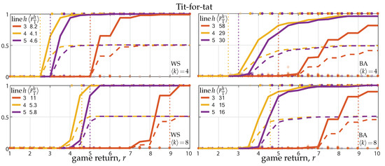
Figure 1.
Invasion and fixation of the tit-for-tat strategy against a population of unconditional defectors. Panels show the fraction of T-agents reached in game rounds starting from a single initial T on WS and BA networks (left and right panels) as a function of the PD return r (average degree and 8 in top and bottoms panels). Solid lines show the average fraction over 100 random initializations (network generation and random placement of the initial T). Dashed lines show the average fraction of cooperative actions, saturating at fixation to 0.5 because of the alternate exploitation triggered by new T-agents with their T-neighbors. Dots show the outcomes of single simulations (T-fraction); transparency is used to show dots accumulation. Colors code the predictive horizon h, from 3 to 5, and the corresponding invasion threshold , averaged over the 100 networks, is reported; the invasion threshold for degree-4 and -8 regular networks are indicated by the vertical dotted lines. The results were obtained for strategy update rate .
Looking at a single panel, the solid curves define the actual invasion and fixation thresholds (the theoretical invasion threshold , averaged over the 100 networks, is systematically larger), so that, for given connectivity ( or 8), cooperation is favored if r is sufficiently increased. Comparing top and bottom panels, we can see network reciprocity. Indeed, the invasion and fixation thresholds both increase by doubling the network connectivity. Note that, in accordance with Corollary 1, the invasion threshold does not always decrease by extending the predictive horizon.
Similar results can be obtained for regular networks, e.g., lattices, rings, and complete networks. Invasion and fixation on regular networks are however ruled by Corollary 2, so the long-term fraction of T-agents jumps from 0 to 1 when r exceeds the invasion thresholds. The thresholds for degree-4 and -8 are marked by dotted lines in the left and right panels in Figure 1.
Comparing left and right panels, we can see the effect of the network’s heterogeneity (single-scale vs. scale-free networks). The effect is quite limited, in agreement with the empirical observations [52,53]. Indeed, although the average invasion threshold of Corollary 1 is much larger for BA networks than for WS networks, the actual thresholds resulting from the simulations are comparable. Looking more closely, it can however be noted that scale-free (BA) networks make invasion easier and fixation more demanding, compared to same-average-degree single-scale (WS) networks. The effect on invasion is due to the skewness of the degree distributions of BA networks toward small degrees (the minimum degree being ), which lowers, on average, the invasion threshold of Theorem 1. The effect on fixation is evidently due to D-hubs, which raise the requirement on r to eventually switch to T.
A secondary effect is due to the fact that, by construction, the degree distribution of our random networks is more heterogeneous (larger variance) the larger is the average degree. As a result, there is no invasion in networks with for r smaller or equal than the invasion threshold for a same-degree regular network (see the dotted vertical lines in the top panels), whereas in networks with (bottom panels) invasion is present in more than 90% of the experiments for r at the dotted threshold.
3.2. Tit-for-two-tats vs. D
In the case of the tit-for-two-tats strategy, against unconditional defection, the expressions for the expected payoffs are reported in Table 4. As in Table 2 for the classical tit-for-tat, we also report the horizon-1 payoff gains and , respectively, expected by a T- and a D-agent when changing strategy. Evidently, the first is zero (if the T-agent i only has DCD and DDD-neighbors) or positive, while the second is negative, confirming that cooperation needs a multi-step predictive horizon.
A substantial difference with respect to the classical tit-for-tat is that the tit-for-two-tats strategy cannot invade from a single agent. Indeed, the single T-agent i classifies all her neighbors as DCD1 after the first game round, so that, if strategy revising, she will compute for all r and h (see Table 4). However, with probability , agent i will not revise her strategy after the first round and she will classify defecting neighbors as DCD after the second round and as DDD later on, hence computing, before any change in her neighborhood, .
Considering all possible realizations of the evolutionary processes, thus including the strategy revision of the initial T-agents after the first round, we can only derive invasion and fixation conditions starting from a pair of connected T-agents.
Theorem 3.
The tit-for-two-tats strategy invades from the agent pair if and only if and
where,, and.
Corollary 3.
The tit-for-two-tats strategy invades from any pair of connected agents if and only if and
where (introduced in Theorem 2) is the largest degree in the network, and .
Note that only a fraction of all possible realizations of the evolutionary processes require in Theorem 3 and Corollary 3, i.e., those in which at least one of the two initial T-agents change to D after the first game round. Neglecting this unfortunate situation (recall that the rate of strategy update is assumed small), the invasion condition from a pair of connected T-agents weakens to the second in Equations (4) and (5) (valid also for ).
More interestingly, we can now consider the invasion condition from a single T-agent, neglecting the -fraction of the realizations in which the agent does not revise strategy after the first round.
Theorem 4.
Assuming agent i does not revise strategy after the first round, the tit-for-two-tats strategy invades from agent i if and only if and
where (introduced in Theorem 1) is the lowest of i-neighbors’ degrees.
Corollary 4.
The tit-for-two-tats strategy invades from any agent, provided she does not revise strategy after the first round, if and only if and
where (introduced in Corollary 1) is the largest of the .
Note that the invasion threshold set by the condition in Equation (7) does decrease monotonically with the length h of the predictive horizon, contrary to the threshold for the classical tit-for-tat, essentially because the tit-for-two-tats agents establish permanent cooperation with their T-neighbors.
Theorem 5.
The tit-for-two-tats strategy monotonically fixates in a network with at least a pair of T-agent if and
where (introduced in Theorem 2) is the largest degree in the network.
Note that the tit-for-two-tats strategy cannot fixate for , independently on the value of the return r. The reason is twofold. For , similarly to the case of the classical tit-for-tat, the coefficient of in equals 2, but also the coefficient of is positive and equal to 1 (see Table 4). Thus, the T-agent i is tempted to change to D if she has enough TCD1- and DCD1-neighbors. Instead of cooperating twice with TCD1-neighbors and being exploited once by DCD1-neighbors in the two rounds of the predictive horizon, it is better to exploit TCD1-neighbors twice and avoid being exploited. The gains per TCD1- and DCD1-neighbor are indeed 2 and 1, respectively. This situation happens, in particular, when the D-agent i is surrounded by a mix of TDD- and DDD-neighbors and r is large enough to induce i to change strategy. Then, as soon as i switches to T and plays C, she updates the classification of TDD- and DDD-neighbors into TCD1 and DCD1, respectively. New T-agent can therefore switch back to D, but only if strategy revising twice in a row. Assuming this does not happen (because of the small rate of strategy change ), fixation is realized also for , under the second condition in Equation (8).
Another related difference, with respect to the case of the classical tit-for-tat, is that the system can reach the state all-D, because isolated T-agents can change to D immediately after getting first exploited by D-neighbors. Being obliged, as T-agents, to cooperate a second time, they prefer to switch to C.
Finally, note that on regular networks (all nodes with same degree k), because , the conditions in Equations (4) and (5) of Theorem 3 and Corollary 3 coincide, so that the latter becomes ‘iff’ and we have the following
Corollary 5.
On regular networks, for , the invasion of the tit-for-two-tats strategy implies its monotonic fixation.
Theorems 3–5 and their corollaries show network reciprocity also in the case of the tit-for-two-tats strategy. As done in Section 3.1, to quantify the actual invasion and fixation thresholds, we ran numerical simulations. Figure 2 shows the results on Watts–Strogatz (WS) and Barabási–Albert(BA) networks (left and right panels) with average degree and (top and bottom panels). As in Figure 1, the solid lines show the long-term fraction of T-agents as a function of the PD return r, averaged over 100 simulations on randomly generated networks and initial conditions. The dashed lines showing the fraction of cooperative actions are however invisible, being indistinguishable (at the scale of the figure) from the corresponding solid lines. Although T-agents do not always cooperate, they establish permanent cooperation with their T-neighbors, thus the defective actions of T-agents essentially occur only at the border of T-clusters and constitute a minor fraction. Consequently, T-agents always cooperate at fixation, i.e., the fixation of the tit-for-two-tats implies the fixation of cooperation.
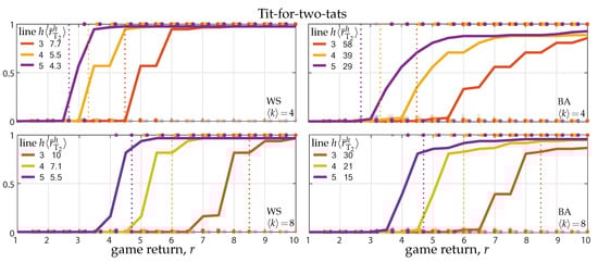
Figure 2.
Invasion and fixation of the tit-for-two-tats strategy against a population of unconditional defectors. Panels show the fraction of T-agents reached in game rounds starting from a single initial T in WS and BA networks (left and right panels) as a function of the PD game return r (average degree and 8 in top and bottom panels). Solid lines show the average fraction over 100 random initializations (network generation and random placement of the initial T). Dots show the outcomes of single simulations; transparency is used to show dots accumulation. Colors code the predictive horizon h, from 3 to 5, and the corresponding invasion threshold , averaged over the 100 networks, is reported; the invasion threshold for degree-4 and -8 regular networks are indicated by the vertical dotted lines. The results were obtained for strategy update rate .
Most of the other observations presented at the end of Section 3.1 also hold for the tit-for-two-tats strategy. Comparing top and bottom panels, we can see network reciprocity, i.e., the invasion and fixation thresholds both increase by doubling the network connectivity. Similar results hold for regular networks (lattices, rings, and complete networks) for which the invasion and fixation threshold are ruled by Corollary 5 and displayed in Figure 2 (for degree-4 and -8) by the vertical dotted lines. Regarding the network’s heterogeneity, the effect it is still quite limited (comparison between single-scale and scale-free networks; left and right panels).
Differently from the classical tit-for-tat, the invasion threshold does decrease monotonically with the length of the predictive horizon, in accordance with Corollary 4 (see the increasing values of the purple, yellow, and red threshold and the left-to-right order of the corresponding curves), confirming the role of the multi-step prediction in the strategy update.
Finally note that the fraction of T-agents does not reach one for large r (this is particularly visible in the right panels). The reason is that we started all simulations from one (randomly placed) T-agent and, accordingly with Theorem 4 and Corollary 4, there is a -probability that the initial T-agent changes to D after the first game round. If this happens to agent i, and r is above the invasion threshold in Equation (6) of Theorem 4, then a neighbor j of i could have changed to T, otherwise the network remains trapped in the absorbing state all-D.
3.3. New-tit-for-two-tats vs. D
In the case of the new-tit-for-two-tats strategy, against unconditional defection, the expressions for the expected payoffs are reported in Table 6. As in the previous cases, we also report the horizon-1 payoff gains and , respectively, expected by a T- and a D-agent when changing strategy. Evidently, the first is zero (if the T-agent i only has DCD-, DCD1-, and DDD-neighbors) or positive, while the second is negative, confirming that cooperation needs a multi-step predictive horizon.
Theorem 6.
The new-tit-for-two-tats strategy invades from agent i if and only if and
where (introduced in Theorem 1) is the lowest of i-neighbors’ degrees.
Corollary 6.
The new-tit-for-two-tats strategy invades from any agent if and
(introduced in Corollary 1) is the largest of the .
Note that the invasion threshold set by the condition in Equation (10) does decrease monotonically with the length h of the predictive horizon. As in the case of the standard tit-for-two-tats, this is due to the permanent cooperation established by T-agents with their T-neighbors.
Theorem 7.
The new-tit-for-two-tats strategy monotonically fixates if and
where (introduced in Theorem 2) is the largest degree in the network.
Note that the new-tit-for-two-tats strategy can fixate also for , provided the game return r is large enough. The reason is that, differently from the two previously analyzed cooperative strategies, TCD1- and DCD1-neighbors no longer tempt the T-agent i to change strategy. By remaining T in the two rounds of the predictive horizon, agent i cooperates twice with TCD1-neighbors and defects twice with DCD1-neighbors, whereas she exploits TCD1-neighbors once by changing to D. The gains per TCD1- and DCD1-neighbor are for and 0, respectively. This situation happens, in particular, when the D-agent i is surrounded by a mix of TDD- and DDD-neighbors and r is large enough to induce i to change strategy. Then, as soon as i switches to T and plays C, she updates the classification of TDD- and DDD-neighbors into TCD1 and DCD1, respectively.
Finally, note that on regular networks (all nodes with same degree k), because , the conditions in Equations (9) and (10) of Theorem 6 and Corollary 6 coincide, so that the latter becomes ‘iff’ and we have the following
Corollary 7.
On regular networks, the invasion of the new-tit-for-two-tats strategy implies its monotonic fixation.
Theorems 6 and 7 and their corollaries show network reciprocity also in the case of the new-tit-for-two-tats strategy. As done for the other two cases, we quantified the actual invasion and fixation thresholds by running numerical simulations. Figure 3 show the results on Watts–Strogatz (WS) and Barabási–Albert(BA) networks (left and right panels) with average degree and (top and bottom panels). As in Figure 2, the solid lines show the long-term fraction of T-agents as a function of the PD return r, averaged over 100 simulations on randomly generated networks and initial conditions, while the dashed lines, showing the fraction of cooperative actions, are indistinguishable from the corresponding solid lines. As for the tit-for-two-tats strategy, new-tit-for-two-tats-agents establish permanent cooperation with their T-neighbors, thus only a minority of T-agents’ actions are defective and the fixation of the T-strategy implies the fixation of cooperation.
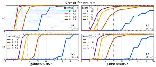
Figure 3.
Invasion and fixation of the new-tit-for-two-tats strategy against a population of unconditional defectors. Panels show the fraction of T-agents reached in game rounds starting from a single initial T in WS and BA networks (left and right panels) as a function of the PD game return r (average degree and 8 in top and bottom panels). Solid lines show the average fraction over 100 random initializations (network generation and random placement of the initial T). Dots show the outcomes of single simulations; transparency is used to show dots accumulation. Colors code the predictive horizon h, from 2 to 5, and the corresponding invasion threshold , averaged over the 100 networks, is reported; the invasion threshold for degree-4 and -8 regular networks are indicated by the vertical dotted lines. The results were obtained for strategy update rate .
Most of the other observations presented at the end of Section 3.1 and Section 3.2 also hold for the new-tit-for-two-tats strategy. Comparing top and bottom panels, we can see network reciprocity, i.e., the invasion and fixation thresholds both increase by doubling the network connectivity. Similar results hold for regular networks (lattices, rings, and complete networks) for which the invasion and fixation threshold are ruled by Corollary 7 and displayed in Figure 3 (for degree-4 and -8) by the vertical dotted lines. Regarding the network’s heterogeneity, the effect it is still quite limited (comparison between single-scale and scale-free networks; left-to-right panels).
Comparing the three types of analyzed cooperative strategies, we can see that the invasion and fixation thresholds in Figure 3 are both lower than those in Figure 1 and Figure 2. The same can be seen to hold between the theoretical thresholds for the new-tit-for-two-tats (Theorem and Corollary 6) and those for the tit-for-tat and of the tit-for-two-tats (Theorems and Corollaries 3 and 1). This is related to the ‘degree’ of reciprocity implemented by the cooperative strategy. The classical tit-for-tat has the highest degree, i.e., the strategy is unforgiving toward defectors; The standard tit-for-two-tats has the lowest, always forgiving the first defection. Both these extrema hinder the evolution of cooperation, the first because it prevents the establishment of permanent cooperation among T-neighbors and the second because it is too exposed to defectors. Our new variant well combines an intermediate reciprocity with the model-predictive horizon. As tit-for-two-tats-agents, new-tit-for-two-tats agents expect to cooperate with all their T-neighbors during the predictive horizon. However, contrary to the former tit-for-two-tats-agents, they avoid being exploited twice in a row, so that, after the first exploitation, they do not predict the cost of the second in the first round of the horizon.
4. Discussion and Conclusions
We implemented and analyzed an EGT model in which the tit-for-tat strategy (T) and unconditional defection (D) face each other in a networked prisoner’s dilemma (PD), under a rational process of strategy update according to which agents compute a prediction of their future income and change strategy (from T to D or vice versa) if they expect a higher payoff. Both our analytic and numerical results show the presence of network reciprocity in this EGT setup. The invasion and fixation thresholds for the T-strategy set by our theorems on the PD return r systematically increase with the connectivity of the network, indicating the complete network as the worst case for the rational evolution of cooperation. The simulations confirm that the actual thresholds (averaged on 100 random networks and initial conditions) increase by doubling the average connectivity of the network, with an effect that is amplified by the length of the predictive horizon.
These results contribute to resolve an inconsistency between the theoretical work on network reciprocity [13,14,19], where the network effect has been found only under imitative evolutionary processes, and the available experiments [50,51,52,53,54,55,56], in which network reciprocity emerged between reciprocal cooperators and rather unconditional defectors who both did not show an imitative behavior. Identifying the rules followed by human subjects to switch between these two emerging strategies is a difficult and ambitious task, which is in any case dependent on the specific experimental setting [51,53,54,61]. Definitely easier is to test a hypothesis on a theoretical model. Our hypothesis is that a multi-step, model-predictive process of strategy update can explain the observed network reciprocity. This has been recently shown true (in [57], coauthored by two of the authors of the present paper) in a model in which the reciprocal behavior of C-agents is introduced in a non-standard way (by allowing T-agents to temporarily abstain from playing with D-neighbors, see the Introduction). The present work has therefore made our hypothesis more robust, by confirming it with the use of the standard form of direct reciprocity—the tit-for-tat strategy.
4.1. Three Versions of the T-strategy
We tested three versions of the T-strategy: the classical one, the more forgiving tit-for-two-tats, and an intermediate variant, which we named new-tit-for-two-tats, in which T-agents play as tit-for-two-tats only when they are ‘new’ T-agents, i.e., when they change strategy from D to T they forgive the first defection from the neighbors who are expected to be T.
Although the classical T-strategy can fixate starting from a single T-agent in any network, provided the game return r is large enough, the fixation of cooperation is typically not obtained, as the pairs of T-neighbors who did not start together as T (at Round 1 or switching together from D to T) alternatively exploit each other. The tit-for-two-tats strategy is specifically designed to avoid this problem, i.e., T-agents establish permanent cooperation with their T-neighbors. It however requires a pair of connected T-agents to invade under a sufficiently high game return. Indeed, a tit-for-two-tats agent with only D-neighbors switches to D when revising her strategy, because, by remaining T, she has to pay the cost of the second exploitation by her D-neighbors. In contrast, once a classical T gets exploited by all her neighbors, she is protected from further defections and remains T when strategy revising (the expected payoffs computed behaving as T and D are both null).
However, the pair of connected T-agents required by the tit-for-two-tats strategy to invade can easily arise because of a D-neighbor of an isolated T-agent i changing to T before the T-agent revises her strategy, provided the game return r is large enough. Under our slow and asynchronous process of strategy update (small probability of strategy revision after each game round), the probability that this indeed happens goes as (shown in [57], Supplementary Material). This can be seen in Figure 2, which shows the average results of simulations initialized with a single T-agent in the network. The fraction of T-agents saturates slightly below one for increasing r, not because the T-agents do not reach fixation, but because of the T-strategy not invading in some of the cases (see the dots showing the outcomes of single simulations).
Despite the above issues, the classical T and the tit-for-two-tats strategies behave rather similarly. Both require a predictive horizon of at least three rounds: the classical T because of the TCD-neighbors of a T-agent, yielding expected payoffs (for h even); behaving as T, because of the alternate exploitation; and r behaving as D, because of a single exploitation in the first round of the predictive horizon in which TCD-neighbors are expected to cooperate (see Table 2). Thus, if , classical T-agents with sufficient TCD-neighbors change to D when revising strategy. Similarly, for , tit-for-two-tats-agents switch to D when surrounded by a sufficient fraction of TCD1 and TCC-neighbors, since they expect the highest payoff by exploiting these neighbors for two consecutive rounds (see Table 4).
As for the invasion and fixation thresholds for , the two strategies behave comparably (compare Figure 1 and Figure 2). The classical T has lower thresholds for h even (e.g., the thresholds for in Figure 1 are lower than those for ). This is again due to the alternate exploitation patterns established by D-agent changing to T, who expect, against their T-neighbors, an equal number of remunerative and costly exploitations for h even, and one extra costly one for h odd. The tit-for-two-tats suffers no difference between h even and odd, and it therefore performs better than the classical T for h odd, in the sense of requiring lower thresholds.
Our new variant, the new-tit-for-two-tats strategy, outperforms the classical T and the tit-for-two-tats on all aspects, being however more complex to implement, as it requires agents to keep track of more information. By playing as tit-for-two-tats once when they change from D to T, T-agents establish permanent cooperation with T-neighbors. Moreover, for , they are not tempted to go back D by TCD1 and TCC-neighbors, who can be exploited only once if changing to D. new-tit-for-two-tats can therefore invade and fixate also for , and the required threshold on r is essentially that of the classical T for . In general, for the same length of the predictive horizon, the invasion threshold of the new-tit-for-two-tats halves the one of the classical T (compare the conditions in Corollaries 1 and 6), and most often invasion implies fixation in simulations, because the (sufficient) conditions we derived for fixation are rather conservative (they actually grant a monotonic growth of the strategy, during which Ts never change to D and Ds connected to Ts sooner or later change to T).
4.2. Comparison with the T-strategy in Dercole et al. (2019)
As described in the Introduction, the model here analyzed is similar to the one proposed and analyzed in [57]. The only conceptual difference is the way in which direct reciprocity is introduced in the T-strategy. This difference however affects the way in which payoffs predictions are computed in the strategy update, and this ultimately makes the implementation and the analysis of the two models quite different.
Direct reciprocity is implemented in [57] by allowing T-agents to temporarily abstain from playing with D-neighbors. More precisely, T-agents always cooperate when playing, but stop playing with a D-neighbor after getting exploited. During the abstention period, they collect no payoff and no information from that link and, at each round, they decide whether to go back playing or not with the probability that the neighbor has revised her strategy ever since the exploitation (the probability is computed in accordance with the rate of strategy update—the model parameter —that is public knowledge to all agents). This is an interesting form of direct reciprocity because it does not force retaliation, i.e., T-agents playing D, as we further underline below in the discussion of the impact of our analyses on applied behavioral science.
The standard and well-recognized way to model direct reciprocity is however the tit-for-tat strategy [3], thus we found it mandatory to use it to confirm the general message put forward in [57] and to make it independent from the adopted form of direct reciprocity. The message, summarized by the title of the present paper, is that direct reciprocity and the multi-step model-predictive process of strategy update together explain network reciprocity in socioeconomic networks.
We have also confirmed two secondary results that emerged in [57]. The first is that both direct reciprocity and the multi-step predictive horizon are necessary for the invasion and fixation of cooperation, and therefore to see network reciprocity. Indeed, cooperation disappears in any network if the T-strategy is replaced by unconditional C or if the length h of the predictive horizon is set to one. The second is the marginal role of the network structure, in agreement with experimental results [52,53], and in contrast with theoretical models based on imitation [20,21,22,23,24,25,26,27,28,29,30,31,32,33,34,35,36], according to which heterogeneous networks should better support cooperation than homogeneous ones with same average connectivity.
Comparing the three variants here analyzed of the tit-for-tat strategy with the A-strategy based on abstention of Dercole et al. [57], we can say that the former implement a stronger form of direct reciprocity than the latter. This is essentially due to the fact that, when a T-agents starts to defect a neighbor, she will keep defecting as long as the neighbor does the same. In contrast, A-agents poll neighbors, from time to time, to seek cooperation, a behavior that is connatural with their C-mood, but that however raises the exploitation risk.
Consequently, an isolated T-agent is not tempted to change to D, whereas isolated A-agents do change whenever they revise their strategy. The invasion of the A-strategy is therefore more demanding, not only in terms of the game return r, but also in terms of the number and connectivity of the initial A-agents. Provided r is large enough to let the D-neighbors of an isolated A-agent to change to A, the probability that a D-neighbor revises before the A-agent goes as (as already discussed above for the tit-for-two-tats strategy after the first round only), so that the A strategy more easily invades from highly connected nodes. This effect is however not visible by comparing the simulations (e.g., our Figure 3 with Figure 2 in [57]), because to make invasion more likely and be able to study network reciprocity, the simulations in [57] start from initial fraction of A-agents (10 agents for networks of 1000 nodes), whereas a single T-agent has been used here. The resulting invasion and fixation thresholds are therefore not comparable. Indeed, they are systematically smaller for the A-strategy because with 10 initial agents the probability that their D-neighbors are connected to more than one A-agents is significant, and this lowers, on average, the value of r required by D-neighbors to change to A.
Nonetheless, we can see that network reciprocity is stronger in the T-strategy because the corresponding invasion and fixation thresholds are much more sensitive to the doubling of the average connectivity than those of the A-strategy. Being direct reciprocity stronger in the T-strategy, we can therefore conclude that the network effect is amplified by the strength of the reciprocal attitude of cooperators.
4.3. Impact on Applied Behavioral Science
We believe that our work has a direct impact on applied behavioral science. We give a plausible explanation for the motivations guiding human subjects in moving from a cooperative to a defective mood and vice versa. Building a model of the society and using it to make short- to mid-term predictions of future payoffs is perhaps the reasonable compromise between the myopic best-response rule to look at the next round only and the impracticable full farsightedness. Although this requires nontrivial cognitive tasks and humans might not be as rational as we assume, we believe that model-predictions are part of the human decision-making processes, possibly as the result of an intuitive, rather than computational, ability.
To confirm this hypothesis, new experiments must be conducted and we think that our work can help the design of the experimental setting. First, before even testing an experimental dataset against a candidate process of strategy update, we must be able to distinguish the cooperative from the defective mood of the subjects, if any mood really does exist. This distinction is not completely clear from the available experiments, in which C and D were the only options and, except the experiment described in [62] about evolving networks, subjects had to chose whether to play C or D with all neighbors at each game round. Consequently, risk-avoiding defections can be easily confused for a defective mood.
It is therefore important, in our opinion, to allow the subjects to act independently with their neighbors and to abstain from playing with selected ones. For example, allowing independent actions for each neighbor has been recently shown to favor cooperation [62], although it is definitely experimentally challenging. Subjects playing C or abstaining with most neighbors could be classified in the cooperative mood; subjects mainly playing D in a defective mood; and a mix of C and D would indicate the absence of a mood. In addition, the mechanisms of direct reciprocity that are most natural to human subjects could be identified.
4.4. Future Directions
Future theoretical extensions of this work could further validate and generalize the general claim of our title. First, a sensitivity analysis, in particular with respect to the update rate and to the length h of the predictive horizon, will help to clarify one of the most critical aspects of the model-predictive process of strategy update. To be able to make simple predictions, our agents assume no strategy change in the neighborhood during the predictive horizon and this requires the update process to be slow compared to the rate of agents’ interaction.
Second, our results could be made more robust by taking into account some degree of uncertainties in the agents’ behavior, e.g., by introducing some probability of strategy change under an expected gain or errors in the computations of predictions.
Finally, although static and sparse networks are the ideal setting for direct reciprocity, as agents repeatedly interact with the same limited number of neighbors, mechanisms to evolve the social ties in feedback with the game outcomes are known to enhance the evolution of cooperation [62,63,64]. It would then be interesting to study our setting on suitable dynamical networks.
Author Contributions
Conceptualization, F.D., F.D.R., and A.D.M.; methodology, F.D., F.D.R., and A.D.M.; software, F.D.R.; formal analysis, A.D.M.; writing, F.D. and A.D.M.; visualization, F.D.R.; and supervision, F.D. All authors have read and agreed to the published version of the manuscript.
Funding
This research received no external funding.
Conflicts of Interest
The authors declare no conflict of interest.
Appendix A. Theorems and Proofs of Results in Section 3
Appendix A.1. Tit-for-tat vs. D
Proof of Theorem 1.
The T-strategy invades from agent i if and only if, starting with only one T-agent in node i, agent i does not first change strategy (), while at least one D-neighbor j is willing to become T () before any change in her neighborhood.
Agent i classifies all her neighbors as DCD after the first game round and, as long as no neighbor does change, as DDD later on. Before any change in her neighborhood, agent i hence computes (both and are zero, according to Table 2 with ).
The D-neighbor j classifies i as TDC after the first round and, as long as i does not change, as TDD later on, all other neighbors are classified DDD as long as they do not change strategy. Before any change in her neighborhood, agent j hence computes (according to Table 2)
Solving for r gives the conditions in Equation (1), in which the neighbor j giving the weakest requirement is considered. □
Proof of Theorem 2.
The T-strategy monotonically fixates if any T-agent i does not change strategy () and any D-neighbor j is willing to become T ().
For any T-agent i, the expression of can be split into three terms, each proportional to , , and (see Table 2). The corresponding coefficients are , respectively, under for both h even and odd, for h even and for h odd, and for h even and for h odd. The most requiring condition is
For any D-agent j, only the sum can positively contribute to (see Table 2) and this occurs under for h even and for h odd. Under this condition, the case for which requires the largest r is , i.e., the case considered in Equation (A1). The condition on r is then formally equivalent to Equation (2), with however replaced by , because any D-agent j must be willing to change strategy.
The most requiring condition to have both and for any is hence the one expressed in Equation (3). □
Appendix A.2. Tit-for-two-tats vs. D
Proof of Theorem 3.
The T-strategy invades from the agent pair if and only if, starting with only two T-agents in nodes i and j, both agents do not first change strategy ( and ), while at least one D-agent l, neighbor of i or j (or both), is willing to become T () before any change in her neighborhood.
Agents i and j classify all their D-neighbors as DCD1 after the first game round and, as long as they remain Ds, as DDD later on. If revising strategy after the first round, agent hence computes
(see Table 4, with and ), whereas she computes
if revising after round before any change in her neighborhood. Solving for r gives the conditions
the first being more restrictive (at least one of and is larger than 1 to have a connected network). The first condition in Equation (4) follows from considering the agent, among i and j requiring the larger r.
If the D-agent l is neighbor of only one of i and j, then, before any change in her neighborhood, she has one TDC1-neighbor after the first round, one TDC-neighbor after the second round, and one TDD-neighbor later on, all other neighbors being classified DDD. Before any change in her neighborhood, agent l hence computes (according to Table 4)
Note that the resulting expression for does not depend on the round after which the strategy revision takes place. Solving for r gives the first part of the second condition in Equation (4) (the first quantity in the min operator), in which the agent l giving the weakest requirement is considered.
If the D-agent l is neighbor of both i and j, then, before any change in her neighborhood, she has two TDC1-neighbors after the first round, two TDC-neighbors after the second round, and two TDD-neighbors later on, all other neighbors being classified DDD. Before any change in her neighborhood, agent l hence computes (according to Table 4)
Again, the round after which l revises strategy is irrelevant and solving for r gives the remaining part of the second condition in Equation (4) (the second quantity in the min operator), in which the agent l giving the weakest requirement is considered. □
Proof of Theorem 4.
The T-strategy invades from agent i if and only if, starting with only one T-agent in node i, agent i does not first change strategy (), while at least one D-neighbor j is willing to become T () before any change in her neighborhood. Agent i classifies all her D-neighbors as DCD1 after the first game round, as DCD after the second, and as DDD later on. Before any change in her neighborhood, and starting from the second round on, agent i hence computes when strategy revising (see Table 4).
The D-neighbor j classifies i as TDC1 after the first round and, as long as i does not change, as TDC after the second round and as TDD later on, all other neighbors being classified DDD as long as they do not change strategy. Before any change in her neighborhood, agent j hence computes as in Equation (A3), so that solving for r and considering the neighbor j giving the weakest requirement on r gives Equation (6). □
Proof of Theorem 5.
The T-strategy monotonically fixates if any T-agent i with at least one T-neighbor does not change strategy () and any D-neighbor j is willing to become T ().
For any T-agent i, the expression of can be split into three terms, each proportional to , , and (see Table 4). The coefficient of the latter is 1, independently of r, so that the case for which requires the largest r is , i.e., agent i just played C with all her D-neighbors after changing from D to T. The remaining neighbor is classified TCD1, so that agent i computes as in Equation (A2). The condition for any T-agent with at least one T-neighbor is hence formally equivalent to the first condition in Equation (4), with however replaced by (i.e., the first condition in Equation (8)).
For any D-agent j, the expression of can be split into three terms, each proportional to , , and (see Table 4). The coefficient of the latter is , independently of r, so that the case for which requires the largest r is , in which agent j computes
Note that the resulting expression for does not depend on the class of the T-neighbor i and coincides with that in Equation (A3). Solving for r hence gives the condition in Equation (7), with however replaced by (i.e., the second condition in Equation (8)). □
Appendix A.3. New-tit-for-two-tats vs. D
Proof of Theorem 6.
The T-strategy invades from agent i if and only if, starting with only one T-agent in node i, agent i does not first change strategy (), while at least one D-neighbor j is willing to become T () before any change in her neighborhood.
Agent i classifies all her neighbors as DCD1 after the first game round and, as long as no neighbor does change, as DDD later on. Before any change in her neighborhood, agent i hence computes (both and are zero, according to Table 6 with ).
The D-neighbor j classifies i as TDC after the first round and, as long as i does not change, as TDD later on, all other neighbors being classified DDD as long as they do not change strategy. Before any change in her neighborhood, agent j hence computes (according to Table 6)
Solving for r gives the condition in Equation (9), in which the neighbor j giving the weakest requirement is considered. □
Proof of Theorem 7.
The T-strategy monotonically fixates if any T-agent i does not change strategy () and any D-neighbor j is willing to become T ().
For any T-agent i, the expression of is proportional to the sum (see Table 6), and the proportionality coefficient is if .
For any D-agent j, the expression of can be split into three terms, each proportional to , , and (see Table 6). The coefficient of the latter is , independently of r, so that the case for which requires the largest r is , in which agent j computes
Note that the resulting expression for does not depend on the class of the T-neighbor i and coincides with that in Equation (A4). Solving for r hence gives the condition in Equation (10), with however replaced by .
The most requiring condition to have both and for any is hence the one expressed in Equation (11). □
References
- Trivers, R.L. The Evolution of Reciprocal Altruism. Q. Rev. Biol. 1971, 46, 35–37. [Google Scholar] [CrossRef]
- Axelrod, R.; Hamilton, W.D. The Evolution of Cooperation. Science 1981, 211, 1390–1396. [Google Scholar] [CrossRef] [PubMed]
- Axelrod, R. The Evolution of Cooperation; American Association for the Advancement of Science: Washington, DC, USA, 2006. [Google Scholar]
- Sigmund, K. The Calculus of Selfishness; Princeton University Press: Princeton, NJ, USA, 2010. [Google Scholar]
- Nowak, M.; Highfield, R. SuperCooperators: Altruism, Evolution, and Why We Need Each Other to Succeed; Simon and Schuster: New York, NY, USA, 2011. [Google Scholar]
- Ocampo-Martinez, C.; Quijano, N. Game-Theoretical Methods in Control of Engineering Systems: An Introduction to the Special Issue. IEEE Control Syst. 2017, 37, 30–32. [Google Scholar]
- Perc, M.; Jordan, J.J.; Rand, D.G.; Wang, Z.; Boccaletti, S.; Szolnoki, A. Statistical physics of human cooperation. Phys. Rep. 2017, 687, 1–51. [Google Scholar] [CrossRef]
- Hofbauer, J.; Sigmund, K. Evolutionary Games and Population Dynamics; Cambridge University Press: Cambridge, UK, 1998. [Google Scholar]
- Perc, M.; Gómez-Gardeñes, J.; Szolnoki, A.; Floría, L.M.; Moreno, Y. Evolutionary dynamics of group interactions on structured populations: A review. J. R. Soc. Interface 2013, 10, 20120997. [Google Scholar] [CrossRef] [PubMed]
- Nowak, M.A. Evolutionary Dynamics; Harvard University Press: Cambridge, MA, USA, 2006. [Google Scholar]
- Szabó, G.; Fath, G. Evolutionary games on graphs. Phys. Rep. 2007, 446, 97–216. [Google Scholar] [CrossRef]
- Nowak, M.A. Five rules for the evolution of cooperation. Science 2006, 314, 1560–1563. [Google Scholar] [CrossRef]
- Nowak, M.A.; May, R. Evolutionary games and spatial chaos. Nature 1992, 359, 826–829. [Google Scholar] [CrossRef]
- Ohtsuki, H.; Hauert, C.; Lieberman, E.; Nowak, M.A. A simple rule for the evolution of cooperation on graphs and social networks. Nature 2006, 441, 502–505. [Google Scholar] [CrossRef]
- Konno, T. A condition for cooperation in a game on complex networks. J. Theor. Biol. 2011, 269, 224–233. [Google Scholar] [CrossRef]
- Allen, B.; Lippner, G.; Chen, Y.T.; Fotouhi, B.; Momeni, N.; Yau, S.T.; Nowak, M.A. Evolutionary dynamics on any population structure. Nature 2017, 544, 227–230. [Google Scholar] [CrossRef] [PubMed]
- Roca, C.P.; Cuesta, J.A.; Sánchez, A. Promotion of cooperation on networks? The myopic best response case. Eur. Phys. J. B 2009, 71, 587. [Google Scholar] [CrossRef]
- Hauert, C.; Doebeli, M. Spatial structure often inhibits the evolution of cooperation in the snowdrift game. Nature 2004, 428, 643–646. [Google Scholar] [CrossRef] [PubMed]
- Lieberman, E.; Hauert, C.; Nowak, M.A. Evolutionary dynamics on graphs. Nature 2005, 433, 312–316. [Google Scholar] [CrossRef]
- Santos, F.C.; Pacheco, J.M. Scale-free networks provide a unifying framework for the emergence of cooperation. Phys. Rev. Lett. 2005, 95, 098104. [Google Scholar] [CrossRef]
- Santos, F.C.; Pacheco, J.M. A new route to the evolution of cooperation. J. Evol. Biol. 2006, 19, 726–733. [Google Scholar] [CrossRef]
- Santos, F.C.; Pacheco, J.M.; Tom, L. Evolutionary dynamics of social dilemmas in structured heterogeneous populations. Proc. Natl. Acad. Sci. USA 2006, 103, 3490–3494. [Google Scholar] [CrossRef]
- Santos, F.C.; Rodrigues, J.F.; Pacheco, J.M. Graph topology plays a determinant role in the evolution of cooperation. Proc. R. Soc. B 2006, 273, 51–55. [Google Scholar] [CrossRef]
- Gómez-Gardeñes, J.; Campillo, M.; Floría, L.M.; Moreno, Y. Dynamical Organization of Cooperation in Complex Topologies. Phys. Rev. Lett. 2007, 98, 108103. [Google Scholar] [CrossRef]
- Ohtsuki, H.; Nowak, M.A. Direct reciprocity on graphs. J. Theor. Biol. 2007, 247, 462–470. [Google Scholar] [CrossRef]
- Poncela, J.; Gómez-Gardeñes, J.; Floria, L.M.; Moreno, Y. Robustness of cooperation in the evolutionary prisoner’s dilemma on complex networks. New J. Phys. 2007, 9, 184. [Google Scholar] [CrossRef]
- Assenza, S.; Gómez-Gardeñes, J.; Latora, V. Enhancement of cooperation in highly clustered scale-free networks. Phys. Rev. E 2008, 78, 017101. [Google Scholar] [CrossRef] [PubMed]
- Gómez-Gardeñes, J.; Poncela, J.; Floría, L.M.; Moreno, Y. Natural selection of cooperation and degree hierarchy in heterogeneous populations. J. Theor. Biol. 2008, 253, 296–301. [Google Scholar] [CrossRef] [PubMed]
- Pusch, A.; Weber, S.; Porto, M. Impact of topology on the dynamical organization of cooperation in the prisoner’s dilemma game. Phys. Rev. E 2008, 77, 036120. [Google Scholar] [CrossRef]
- Santos, F.C.; Santos, M.D.; Pacheco, J.M. Social diversity promotes the emergence of cooperation in public goods games. Nature 2008, 454, 213–216. [Google Scholar] [CrossRef]
- Devlin, S.; Treloar, T. Evolution of cooperation through the heterogeneity of random networks. Phys. Rev. E 2009, 79, 016107. [Google Scholar] [CrossRef]
- Devlin, S.; Treloar, T. Cooperation in an evolutionary prisoner’s dilemma on networks with degree-degree correlations. Phys. Rev. E 2009, 80, 026105. [Google Scholar] [CrossRef]
- Floría, L.; Gracia-Lázaro, C.; Gómez-Gardenes, J.; Moreno, Y. Social network reciprocity as a phase transition in evolutionary cooperation. Phys. Rev. E 2009, 79, 026106. [Google Scholar] [CrossRef]
- Perc, M. Evolution of cooperation on scale-free networks subject to error and attack. New J. Phys. 2009, 11, 033027. [Google Scholar] [CrossRef]
- Cardillo, A.; Gómez-Gardeñes, J.; Vilone, D.; Sánchez, A. Co-evolution of strategies and update rules in the prisoner’s dilemma game on complex networks. New J. Phys. 2010, 12, 103034. [Google Scholar] [CrossRef]
- Débarre, F.; Hauert, C.; Doebeli, M. Social evolution in structured populations. Nat. Commun. 2014, 5, 3409. [Google Scholar] [CrossRef] [PubMed]
- Nowak, M.A.; Sigmund, K. Evolution of indirect reciprocity by image scoring. Nature 1998, 393, 573–577. [Google Scholar] [CrossRef] [PubMed]
- Hamilton, W.D. The genetical evolution of social behaviour. J. Theor. Biol. 1964, 7, 1–16. [Google Scholar] [CrossRef]
- Wilson, D.S. A general theory of group selection. Proc. Natl. Acad. Sci. USA 1975, 72, 143–146. [Google Scholar] [CrossRef] [PubMed]
- Jansen, V.A.; van Baalen, M. Altruism through beard chromodynamics. Nature 2006, 440, 663–666. [Google Scholar] [CrossRef] [PubMed]
- Fletcher, J.A.; Doebeli, M. A simple and general explanation for the evolution of altruism. Proc. R. Soc. Lond. B 2009, 276, 13–19. [Google Scholar] [CrossRef]
- Bolton, G.E.; Ockenfels, A. A theory of equity, reciprocity and competition. Am. Econ. Rev. 2000, 90, 166–193. [Google Scholar] [CrossRef]
- Capraro, V. A model of human cooperation in social dilemmas. PLoS ONE 2013, 8, e72427. [Google Scholar] [CrossRef]
- Capraro, V.; Rand, D.G. Do the Right Thing: Experimental evidence that preferences for moral behavior, rather than equity or efficiency per se, drive human prosociality. Judgm. Decis. Mak. 2018, 13, 99–111. [Google Scholar] [CrossRef]
- Vanberg, V.J.; Congleton, R.D. Rationality, Morality, and Exit. Am. Polit. Sci. Rev. 1992, 86, 418–431. [Google Scholar] [CrossRef]
- Batali, J.; Kitcher, P. Evolution of altriusm in optional and compulsory games. J. Theor. Biol. 1995, 175, 161–171. [Google Scholar] [CrossRef] [PubMed]
- Boyd, R.; Gintis, H.; Bowles, S.; Richerson, P.J. The Evolution of Altruistic Punishment. Proc. Natl. Acad. Sci. USA 2003, 100, 3531–3535. [Google Scholar] [CrossRef] [PubMed]
- Dercole, F.; De Carli, M.; Della Rossa, F.; Papadopoulos, A.V. Overpunishing is not necessary to fix cooperation in voluntary public goods games. J. Theor. Biol. 2013, 326, 70–81. [Google Scholar] [CrossRef] [PubMed]
- Semmann, D. Conditional cooperation can hinder network reciprocity. Proc. Natl. Acad. Sci. USA 2012, 109, 12846–12847. [Google Scholar] [CrossRef] [PubMed]
- Grujić, J.; Fosco, C.; Araujo, L.; Cuesta, J.A.; Sánchez, A. Social experiments in the mesoscale: Humans playing a spatial prisoner’s dilemma. PLoS ONE 2010, 5, e13749. [Google Scholar] [CrossRef]
- Grujić, J.; Röhl, T.; Semmann, D.; Milinski, M.; Arne, T. Consistent Strategy Updating in Spatial and Non-Spatial Behavioral Experiments Does Not Promote Cooperation in Social Networks. PLoS ONE 2012, 7, e47718. [Google Scholar] [CrossRef]
- Gracia-Lázaro, C.; Ferrer, A.; Ruiz, G.; Tarancón, A.; Cuesta, J.A.; Sánchez, A.; Moreno, Y. Heterogeneous networks do not promote cooperation when humans play a Prisoner’s Dilemma. Proc. Natl. Acad. Sci. USA 2012, 109, 12922–12926. [Google Scholar] [CrossRef]
- Gracia-Lazaro, C.; Cuesta, J.A.; Sanchez, A.; Moreno, Y. Human behavior in Prisoner’s Dilemma experiments suppresses network reciprocity. Sci. Rep. 2012, 2, 1–4. [Google Scholar] [CrossRef]
- Grujić, J.; Gracia-Lazaro, C.; Milinski, M.; Semmann, D.; Traulsen, A.; Cuesta, J.A.; Moreno, Y.; Sanchez, A. A comparative analysis of spatial Prisoner’s Dilemma experiments: Conditional cooperation and payoff irrelevance. Sci. Rep. 2014, 4, 4615. [Google Scholar] [CrossRef]
- Rand, D.G.; Nowak, M.A.; Fowler, J.H.; Christakis, N.A. Static network structure can stabilize human cooperation. Proc. Natl. Acad. Sci. USA 2014, 111, 17093–17098. [Google Scholar] [CrossRef]
- Li, X.; Jusup, M.; Wang, Z.; Li, H.; Shi, L.; Podobnik, B.; Stanley, H.E.; Havlin, S.; Boccaletti, S. Punishment diminishes the benefits of network reciprocity in social dilemma experiments. Proc. Natl. Acad. Sci. USA 2018, 115, 30–35. [Google Scholar] [CrossRef] [PubMed]
- Dercole, F.; Della Rossa, F.; Piccardi, C. Direct Reciprocity and Model-Predictive Rationality Explain Network Reciprocity over Social Ties; Scientific Report; Nature Publishing Group: London, UK, 2019. [Google Scholar]
- DiMeglio, A.; Dercole, F.; Della Rossa, F. Direct reciprocity and model-predictive rationality: A setup for network reciprocity over social ties. In Proceedings of the 2019 18th European Control Conference (ECC), Naples, Italy, 25–28 June 2019; pp. 1531–1536. [Google Scholar]
- Grilo, C.; Luís, C. Effects of asynchronism on evolutionary games. J. Theor. Biol. 2011, 269, 109–122. [Google Scholar] [CrossRef] [PubMed]
- Boccaletti, S.; Latora, V.; Moreno, Y.; Chavez, M.; Hwang, D.H. Complex networks: Structure and dynamics. Phys. Rev. 2006, 424, 175–308. [Google Scholar] [CrossRef]
- Traulsen, A.; Semmann, D.; Sommerfeld, R.D.; Krambeck, H.J.; Milinski, M. Human strategy updating in evolutionary games. Proc. Natl. Acad. Sci. USA 2010, 107, 2962–2966. [Google Scholar] [CrossRef]
- Melamed, D.; Harrell, A.; Simpson, B. Cooperation, clustering, and assortative mixing in dynamic networks. Proc. Natl. Acad. Sci. USA 2018, 115, 951–956. [Google Scholar] [CrossRef]
- Perc, M.; Szolnoki, A. Coevolutionary games—A mini review. BioSystems 2010, 99, 109–125. [Google Scholar] [CrossRef]
- Fehl, K.; van der Post, D.J.; Semmann, D. Co-evolution of behaviour and social network structure promotes human cooperation. Ecol. Lett. 2009, 14, 546–551. [Google Scholar] [CrossRef]
© 2020 by the authors. Licensee MDPI, Basel, Switzerland. This article is an open access article distributed under the terms and conditions of the Creative Commons Attribution (CC BY) license (http://creativecommons.org/licenses/by/4.0/).