Measuring and Comparing Two Kinds of Rationalizable Opportunity Cost in Mixture Models


Department of Economics, Mail Stop 922, The University of Toledo, University Hall, Toledo, OH 43606, USA
Games 2020, 11(1), 1; https://doi.org/10.3390/g11010001
Submission received: 23 September 2019
/
Revised: 30 October 2019
/
Accepted: 4 November 2019
/
Published: 19 December 2019
(This article belongs to the Special Issue The Empirics of Behaviour under Risk and Ambiguity)
Abstract
:In experiments of decision-making under risk, structural mixture models allow us to take a menu of theories about decision-making to the data, estimating the fraction of people who behave according to each model. While studies using mixture models typically focus only on how prevalent each of these theories is in people’s decisions, they can also be used to assess how much better this menu of theories organizes people’s utility than does just one theory on its own. I develop a framework for calculating and comparing two kinds of rationalizable opportunity cost from these mixture models. The first is associated with model mis-classification: How much worse off is a decision-maker if they are forced to behave according to model A, when they are in fact a model B type? The second relates to the mixture model’s probabilistic choice rule: How much worse off are subjects because they make probabilistic, rather than deterministic, choices? If the first quantity dominates, then one can conclude that model a constitutes an economically significant departure from model B in the utility domain. On the other hand, if the second cost dominates, then models a and B have similar utility implications. I demonstrate this framework on data from an existing experiment on decision-making under risk.
Keywords:
mixture model; expected utility; rank dependent expected utility; rationalizable opportunity cost; absolute welfare costJEL Classification:
D81; C51; C52; C111. Introduction
Experimental and behavioral economists have largely embraced the idea that there could be more than one process driving behavior in our experiments. Whether it be decision-making under risk (e.g., [1,2]), discounting [3], or choice bracketing [4], to name but a few, we have generally found that our data are better modeled using mixture models [1], rather than assuming that one model of decision-making is generating all of our data. Mixture models assume that subjects can be heterogeneous not just in the parameters that enter subjects’ utility functions, but also the form of the utility functions themselves. Such analysis typically focuses on the “mixing probabilities”, which are the fractions of subjects or decisions1 that are best characterized by one of a list of assumed models. For example, Harrison and Rutström [1] assume that decisions in their experiment are made using either an Expected Utility objective function, or a Prospect Theory objective function, and estimate that approximately 51% of decisions were made using an Expected Utility objective function, and the remainder with a Prospect Theory objective function. If this probability is statistically different from zero and one, the researcher then concludes that both models are important.
However, when used on experimental data, such mixture models are not just models for predicting or “explaining” choices. They are also models of optimization. For example, the expected utility types in Harrison and Rutström [1] are assumed to be maximizing an Expected Utility objective function, and the Prospect Theory types are assumed to be maximizing a Prospect Theory objective function. Hence, while it is of course useful to know the prevalence of each model in our data, we can also evaluate whether one model under consideration constitutes an economically significant departure in utility from another. Consider, for instance, two models labeled B (the “baseline”) and A (the “alternative”), and we are concerned that we may be classifying subjects as A-types when they are in fact B-types, because our decisions based on our estimates will affect the welfare of these individuals. Such a mis-classification could be mostly inconsequential if models A and B only made different predictions about choices in situations where the subject is (approximately) indifferent between her choices. On the other hand, if A and B implied different optimal courses of action for subjects when they had a strong preference for one of these actions, then policy prescriptions made following this mis-classification could have adverse welfare effects.
To illustrate, consider designing a national health insurance program. Suppose that individuals begin with initial wealth of $1, but may lose all of it due to heath expenses. There are two states of the world. In a “healthy” state, which occurs with probability p, individuals have no medical expenses. With remaining probability , individuals are “sick”, and incur $1 in medical expenses. We seek to determine whether full, actuarially fair insurance is welfare-improving compared to a situation without any insurance, and then implement the best policy: full or no insurance. Insurance guarantees wealth of in both states. We are, however, uncertain about whether the individuals’ preferences are better represented by Expected Utility (EU) Theory, or Rank Dependent Expected Utility (RDEU) Theory [5]. Assuming that the individuals are the EU type, then as long as we know that they are risk-averse, they would prefer to be insured rather than not. a special case of this is shown in Figure 1. The yellow line shows how the certainty equivalent for an EU type with utility over wealth of being uninsured varies with probability p, and the black curve shows the certainty equivalent if this individual receives full, actuarially fair insurance. Since the black curve is above the yellow line, these individuals are better off with insurance, no matter what their probability of being sick. Hence, if we were certain that all people were risk-averse EU types, then the program would be welfare-improving.
However if people are RDEU types, then probabilities enter into their preferences differently. Relative to the EU type, these people could put less weight on the probability of being in the sick state, and therefore may have uninsured certainty equivalents that look like the red line in Figure 1. Here I use the same utility over money, , and the probability weighting function in Equation (12), with parameter . These people would only prefer full insurance to no insurance for p greater than about 0.34. As a policy-maker, for smaller values of p we would therefore implement the program only if we believed people had Expected Utility preferences, and not implement the policy if we believed people had Rank Dependent Expected Utility preferences. The consequence of this is shown by the blue curve in Figure 1, which shows how much worse off (change in certainty equivalent) an Expected Utility individual is made, if the policy-maker based their decisions on the RDEU model. This is the mis-classification error: if p is small and we base our policy decision on the red line (RDEU) when individuals’ preferences are in fact represented by the yellow line (EU), then we could have made people better off. On the other hand, there is no such consequence (for these parameters, at least), of incorrectly assuming RDEU preferences for larger values of p.
In this paper, I develop a framework for quantifying the consequences of such a mis-classification. In particular, I quantify the Rationalizable Opportunity Cost (ROC) [6] associated with the alternative model. One can think of this cost as a lower bound of the additional cognitive cost required to use the baseline model, assuming that the baseline model truly represents the subject’s preferences. In the example above and in Figure 1, assume instead that individuals themselves are choosing whether or not to purchase this insurance. If their preferences are actually EU, then buying insurance is optimal for all values of p. Therefore, if they are instead making decisions according to the RDEU model, then they could be better off by the height of the blue curve, which is the difference in certainty equivalents. This difference is the rationalizable opportunity costs of the RDEU model: if using the EU model to make decisions incurred an additional cognitive cost of at least than this rationalizable opportunity cost, then it would be better for the decision-maker to use the RDEU model.
I compare these costs to the Absolute Welfare Cost (AWC) of the probabilistic choice process [7]. This second cost can be interpreted as the rationalizable opportunity cost associated with making probabilistic choices (e.g., logit), instead of making deterministic choices. That is, by behaving probabilistically, rather than deterministically, individuals choose their optimal action with probability strictly less than one, and hence if the opportunity cost of behaving deterministically is greater than the AWC, it is better to behave probabilistically. If probabilistic choices constitute larger costs than do model mis-classifications, then it is likely that the models only prescribe different actions when the baseline type is nearly indifferent between actions. Alternatively, if the mis-classification costs (ROC) are larger, one can interpret this as the models having substantially different implications for utility.
These costs are calculable within the existing framework of structural mixture models as applied to economic experiments. In the remainder of this paper, I develop a framework for calculating them, then demonstrate this framework by applying it to an existing experiment [8]. In this instance, I find that while the vast majority of subjects are estimated to behave according to Rank Dependent Expected Utility theory, subjects’ rationalizable opportunity costs of the RDEU model are generally small when compared to the absolute welfare costs of probabilistic choice: for the Hey [8] experiment, while RDEU decisions may look quite different to EU decisions, Rank Dependent Expected Utility is not substantially different to Expected Utility.
2. Measuring Departures in Utility from a Baseline Model
Mixture models in experiments typically assume that people might make different decisions when faced with the same choice set for three reasons. These reasons are not all unique to mixture models, however I outline them all below in order to characterize two sources of heterogeneity in decisions that I wish to compare, and one that I need to account for. These reasons are:
- They use different objective functionals to make their decisions: e.g., some decisions may be made using Expected Utility theory, and others using Prospect Theory. This is the “mixture” part of the mixture model: the econometrician assumes that there is more than one process generating their data, and sets out to estimate the fraction of the data that are generated by each process.
- Their decisions are noisy: even if two people have the same preferences and use the same objective function, they choose the action that maximizes their objective function with probability less than one. This part of the econometric specification has (at least) two interpretations. It can be motivated through a belief that subjects make mistakes. It can also be interpreted as a component of utility that is random.2
- They have different preferences, conditional on having the same objective functional: e.g., one individual may be more risk-averse than another.
I seek to quantify the economic significance of the first and second reasons. That is, subjects’ decisions could be different due to differences in their objective functionals (reason 1), probabilistic choice (reason 2), or for the purposes of this analysis, nuisance parameters (reason 3).
2.1. A Classification of Behavior
Let one of the types under consideration in the mixture model be the “baseline” type. Reasonable choices for this could be one that satisfies some generally agreed-upon choice axioms, or the model with the fewest parameters (especially if the models are nested). The second column of Table 1 shows some suggested choices for this baseline model considered in existing experiments. Let be this objective function for subject i, where L is an element of i’s choice set. Hence, when presented with choice set , i chooses:
As outlined above, mixture models permit departures from (1) in two distinct ways. Due to Reason 1, i may use an objective function that is not . Let this alternative function be . That is, a subject with objective function will instead seek to choose:
Subjects are also assumed to behave probabilistically (reason 2), also a departure from maximizing , which means that all elements in the choice set, not just the ones that satisfy (1) or (2), are chosen with positive probability. Let be the probability (mass or density, depending on whether is discrete or continuous, respectively) that i chooses element L from their choice set. is implicitly a function of either or , as it maps utilities associated with each element of into a probability distribution over . Popular specifications for these are summarized in the rightmost column Table 1, and in Machina [13].
Table 2 outlines this modeling framework for decisions. Mixture models assume that decisions come from the leftmost column of this table. That is, decisions are assumed to be generated by noisy maximization of either the baseline or alternative model, which I denote BP and AP respectively. The other columns of this table describe useful counterfactual cases for my analysis. The second column describes behavior that would have occurred if one shut down the probabilistic component of subjects’ choices. That is, a subject who is “Baseline-Deterministic” (BD) always chooses the action that maximizes , rather than just being more likely to take this action.
2.2. Rationalizable Opportunity Cost of Using the Alternative Model
Suppose the econometrician estimates two models: a pooled model that assumes all decisions conform to the baseline probabilistic model, and a mixture model that assumes decisions could be generated from either the Baseline- or Alternative-Probabilistic models. Suppose further that the econometrician concludes, through appropriate statistical tests, that the mixture model performs statistically better than the baseline model on its own. The next step of the analysis could be to determine whether the mixture model is economically different to the pooled model.
I approach this second problem by quantifying the economic consequences of mis-classifying decisions as coming from the alternative model, when they are in fact from the baseline model.3 In particular, I seek to quantify the rationalizable opportunity cost [6] of a subject making decisions according to the alternative model, when in fact their preferences are better represented by the baseline model.
Let denote the probability distribution over actions in the choice set associated with subject i using the Baseline model and probabilistic choice (i.e., type BP). Similarly, denotes subject i’s probabilistic choice conditional on being the Alternative type (type AP).
To illustrate, consider again the health insurance example used in the introduction, but instead allow people to themselves choose between either having full insurance or not. In this situation, the decision-maker’s choice set is . If individuals use a logit probabilistic choice rule, then the probability that they choose full insurance conditional on being a Baseline, EU type is:
where measures decision-makers’ sensitivity to payoff differences. Likewise, if individuals are using the Alternative, RDEU model, then they will choose insurance according to:
Individual i’s rationalizable opportunity cost for the alternative model, measured as a difference in certainty equivalents, is:
where is subject i’s certainty equivalent of lottery over their choice set, evaluated using the baseline objective function. Figure 2 shows the certainty equivalents in the insurance example, setting , associated with behaving according to the Baseline-Probabilistic (EU) and Alternative-Probabilistic (RDEU) models, assuming that individuals’ preferences are EU. It is optimal for the EU type to choose full insurance, so as choice precision becomes larger, the EU type is more likely to choose insurance. On the other hand, using the RDEU model under-states the probability of being sick, and so results in lower welfare if preferences are truly represented by the Baseline EU model.4 can be seen on Figure 2 as the vertical distance between the yellow (Baseline) and red (Alternative) lines. That is, holding probabilistic choice constant, what is the individual’s opportunity cost of using the Alternative model, assuming that their preferences are actually represented by the Baseline model?
2.3. Absolute Welfare Cost of Probabilistic Choice
While (5) speaks to the economic significance of the alternative model, holding probabilistic choice constant, it is also useful to compare this to the component of subjects’ utility that we are not modeling through differences between the models. That is, one interpretation of the probabilistic choice rule is that instead of maximizing directly, subjects in fact maximize . Hence, (or if i is the alternative type) is the part of the decision-making process that we are formally modeling, and is the residual, the component of utility that the econometrician does not model explicitly. If is on average small relative to , then one could conclude that the two types are explaining substantial differences in utility. Alternatively, if is large, then the un-modeled component of utility dominates, and so adding the alternative model does not explain much more of subjects’ utility than does the baseline model on its own.
To this end, I also compute the Absolute Welfare Cost (AWC, [7]) of probabilistic choice, which is the rationalizable opportunity cost of probabilistic choice.5 Specifically, I compute the certainty equivalents associated with following the Baseline-Deterministic (BD) decision rule, and the Baseline-Probabilistic (BP) decision rule. The difference between these measures the rationalizable opportunity cost of using probabilistic choice:
This quantity can be seen in Figure 2 as the vertical distance between the yellow line (Baseline, EU), and the maximum of this yellow line. That is, if behaving deterministically incurred an additional cognitive cost of or greater, then individual i could not be made better off by behaving deterministically.
2.4. Total Rationalizable Opportunity Cost
As subjects can behave differently to the baseline-deterministic model for two reasons, it is also useful to compute the total rationalizable opportunity cost of both of these together:
in terms of Figure 2, this quantity is the vertical distance between the red line (RDEU, alternative), and the maximum value of the yellow line (EU, baseline). For this example as choices become more precise (larger ), increases, and a larger fraction of it is attributable to differences in the objective functionals (). Alternatively, if the Alternative-Probabilistic model prescribed approximately the same distribution of choices as the Baseline-Probabilistic model, then would dominate for all but the largest values of .
2.5. Additional Considerations
For most models of choice under risk, the units of utility are not easy to interpret, both within and between subjects. Certainty equivalents, on the other hand, convert these into units of dollars, or other currency, that are easily comparable between subjects, and have context outside of the laboratory. For this analysis, one can interpret a certainty equivalent of following an estimated probabilistic decision rule as “the individual would be indifferent between following the decision rule, and being turned away at the beginning of the experiment with certain amount ” (ignoring cognitive costs, opportunity cost of time, etc.). While certainty equivalents are commonly used for experimental data (See for example Harrison et al. [11], and Bland [4]), it is worthwhile considering alternative measures of welfare, which in principle could be used for similar analysis.
Another common welfare measure is willingness to pay (e.g., Elabed and Carter [14]). In principle, this analysis could be done by calculating the willingness to pay to (i) behave according to the baseline model instead of the alternative (similar to ), and (ii) make deterministic choices using the baseline model, instead of probabilistic choices (similar to ). However popular parameterizations of utility functions in mixture models do not make this feasible. For example, for the popular CRRA specification , consider a lottery that pays $1 with probability 50%, and zero otherwise. The certainty equivalent of this lottery is , which exists for all allowable parameter values. However willingness to pay is computed by solving : either one must assume an initial positive wealth level, modify the experiment so that all payoffs are strictly positive, or we cannot calculate this.
Alternatively, instead of measuring welfare in money, one could express it in uncertainty equivalents [15]. Suppose that prizes in an experiment were on the interval , then the uncertainty equivalent q of lottery L is the probability that makes the individual indifferent between lottery L and the lottery that pays with probability q and with probability . Like certainty equivelents, this measure is easy to calculate from mixture models,6 and is comparable between subjects. I do not use it in my analysis in the next section, although it is certainly appropriate to do so in situations where probability has a more intuitive interpretation than money (e.g., if prizes are not money).
One concern about all of these measures is the treatment of compound risk. Subjects in laboratory experiments usually make many payoff-relevant decisions, and so appropriate treatment of the Reduction of Compound Lotteries assumption is important. Since Expected Utility Theory assumes Reduction of Compound Lotteries, then evaluating certainty equivalents, or other welfare measures, based on the lottery induced by the subject following a decision rule for the entire experiment could be appropriate. Certainty equivalents of this tell us the cash amount that would make the subject indifferent between being paid the certainty equivalent for sure, and being given the lottery induced by their decision rule and the random payment process of the experiment. That is, for a binary choice experiment, this induced lottery is equivalent to the simple lottery, characterized as a vector of probabilities over its prizes:
where is a vector of probabilities over the experiment’s possible prizes describing the probability of winning each prize if lottery is chosen for the tth decision. On the other hand, other models do not assume Reduction of Compound Lotteries, and so this induced lottery is not appropriate. Instead, in these situations, one could evaluate certainty equivalents for single decisions in isolation (again, see Harrison et al. [11] for an example of this).
Although I discuss the Baseline and Alternative models as prescribing deterministic choices if the probabilistic component of choice is removed, this framework can include models that permit deliberate randomization (e.g., Agranov and Ortoleva [16]). For example, if the alternative model prescribed deliberate randomization, then this would be reflected in (the alternative type’s action space would have to be changed to probabilities over the experiments actions, rather than the actions themselves). If the baseline type remains EU, then can be interpreted as the rationalizable opportunity cost of deliberate randomization, and is the rationalizable opportunity cost of probabilistic choice.
3. Application
3.1. Data and Econometric Models
I demonstrate how to calculate these rationalizable opportunity costs using existing experimental data collected originally by Hey [8], and studied subsequently by Moffatt [17] and Conte et al. [2]. I choose to analyze this experiment because its design is similar to many other experiments of decision-making under risk, in that subjects made multiple binary choices between lotteries over money, without adding complexity in areas such as the framing of gains and losses (e.g., Harrison and Rutström [1]), or presenting lotteries over both simple and compound risk (e.g., the “1-in-40” treatment of Harrison et al. [11]). For this experiment, subjects each made 500 binary lottery decisions. Each lottery had the same four prizes: £0, £50, £100, and £150, but differed in the probabilities assigned to each prize.7 One decision was randomly chosen for payment.
I mostly follow the econometric model reported in Conte et al. [2], who use these data to estimate the fraction of subjects who behave according to expected utility theory (EU), which I assume to be the baseline model, and Rank Dependent Expected Utility (RDEU) theory [5], the alternative model. As there were ever only four prizes in any lottery, subject i’s objective function, if they are an EU type, is:
where is the probability of wining prize in lottery L, and is utility of certain amount , with risk-aversion parameter . Hence, when presented with a choice between lotteries and , a Baseline-Deterministic participant would choose if and only if .8 As assumed by Conte et al. [2] I normalize payoffs by dividing prizes by the maximum monetary prize (),9 and estimate the constant relative risk aversion (CRRA) utility function:
Note that as increases, subjects become less risk averse.
If instead subject i is RDEU, they weight probabilities differently to the EU model, which is modeled as:
where are the probabilities weighted according to the function:10
As with Conte et al. [2], I rank prizes from lowest to highest, i.e., , , and so on. The model would have different implications if rankings were reversed.
At this point, both models and are specified. It remains to specify the probabilistic component of decisions. In most of their specifications, Conte et al. [2] model subjects’ probabilistic implementation of their decision rule as Fechnerian errors, which I maintain here. When faced with a choice between lotteries and , they attempt to evaluate , but this is disturbed by an iid error term, which means they choose the lottery that maximizes . Alternatively, if one is not comfortable with being a mistake, one can interpret it as the component of the objective function that is not explicitly modeled by the econometrician. Assuming that results in probit errors:
where is the standard normal cumulative distribution function. I maintain the assumption that the s are independent, mean-zero normal draws, but do not impose that the variance of these errors is constant across subjects (i.e., ) or within types. This restriction is almost universally used for mixture model estimation from experimental data,11 however it is not suitable for my analysis. This is because I wish to quantify the importance of the alternative model relative to probabilistic choice. It is therefore important that my results for one subject are not driven by assuming that subjects are homogeneous along this dimension.
As described above, each individual’s behavior is characterized by three parameters: . While it is in principle possible to estimate these parameters subject-by-subject, I opt for hierarchical specification for the individual-level parameters:
is a latent probability weighting parameter that is used only if subject i uses the RDEU model.
I estimate this model making the same assumption about mixing as Conte et al. [2]: subjects are assumed to make all of their decisions with either the EU model, or the RDEU model.12
where () indicates that subject i uses the EU (RDEU) model. That is, a subject makes all of her decisions using the EU model with probability , and all of them using the RDEU model with probability .
This econometric specification differ from that estimated in Conte et al. [2] in the following notable dimensions:
- The above specification does not assume subjects have the same decision error variance (i.e., ), while Conte et al. [2] assume that is type-specific, instead of decision-specific. I relax their assumption here as I am directly interested in the economic significance of this variable at the subject level.
- Conte et al. [2] includes decision trembles (not model trembles) in addition to probit errors. I exclude these trembles for simplicity of exposition, but in principle they could be included in the probabilistic choice model.
- Conte et al. [2] allow the distribution of subjects’ parameters to depend on their type. For simplicity, I assume that they are all drawn from the same multivariate normal distribution, with simply not being used if they are the EU type.
3.2. Results
I assign priors to this model’s population-level parameters (, , and ), and simulate its posterior distribution using a Markov chain described in Appendix B. Table 3 shows posterior means and standard deviations of the estimated population-level parameters in the mixture model, respectively. The variable of interest to most practitioners has historically been , the fraction of subjects or decisions using the Baseline model, in this case EU. One’s conclusion from this Table is clear: the vast majority of subjects are best characterized by the RDEU model. I estimate that only 3% of subjects are expected utility types.13 Furthermore, a one-sided 95% Bayesian credible region places an upper bound on this fraction of 9.6%. On the individual level, Figure 3 shows the posterior probability that each subject is the EU (baseline) type. In agreement with the population estimates reported in Table 3, the majority of these credible regions only cover probabilities less than than 20%. Focusing on decisions alone, this is strong evidence against the baseline model, if we had to pick one.
Figure 4 shows the extent of probabilistic choice. As is difficult to interpret on its own, I transform this variable into its implied probability of choosing when , which corresponds approximately to the average utility difference of a risk-neutral subject.14 While a large fraction of subjects choose their utility-maximizing lottery with probability close to one in this case, approximately 30% of subjects would choose the less valuable lottery with probability at least 5%.
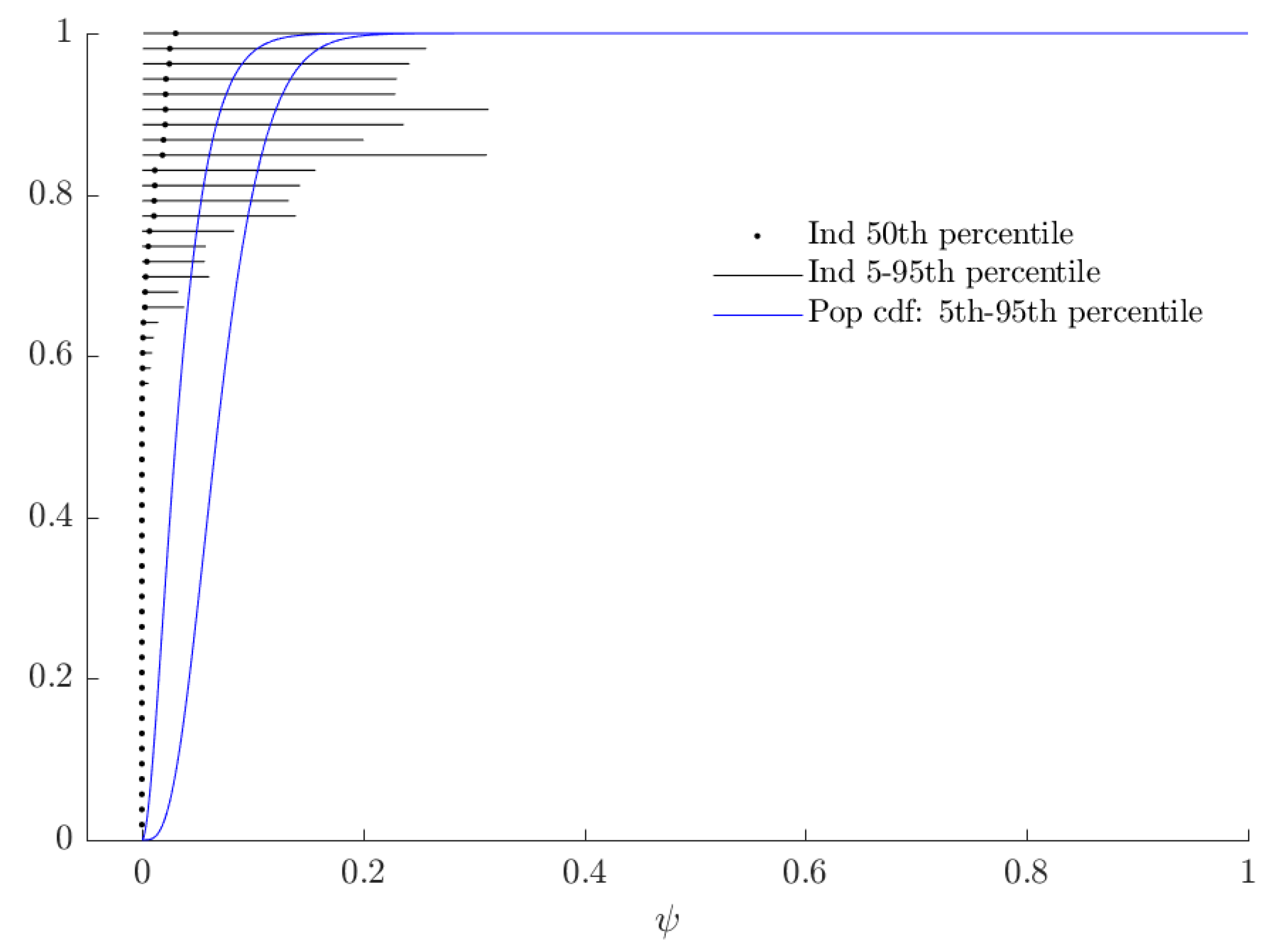
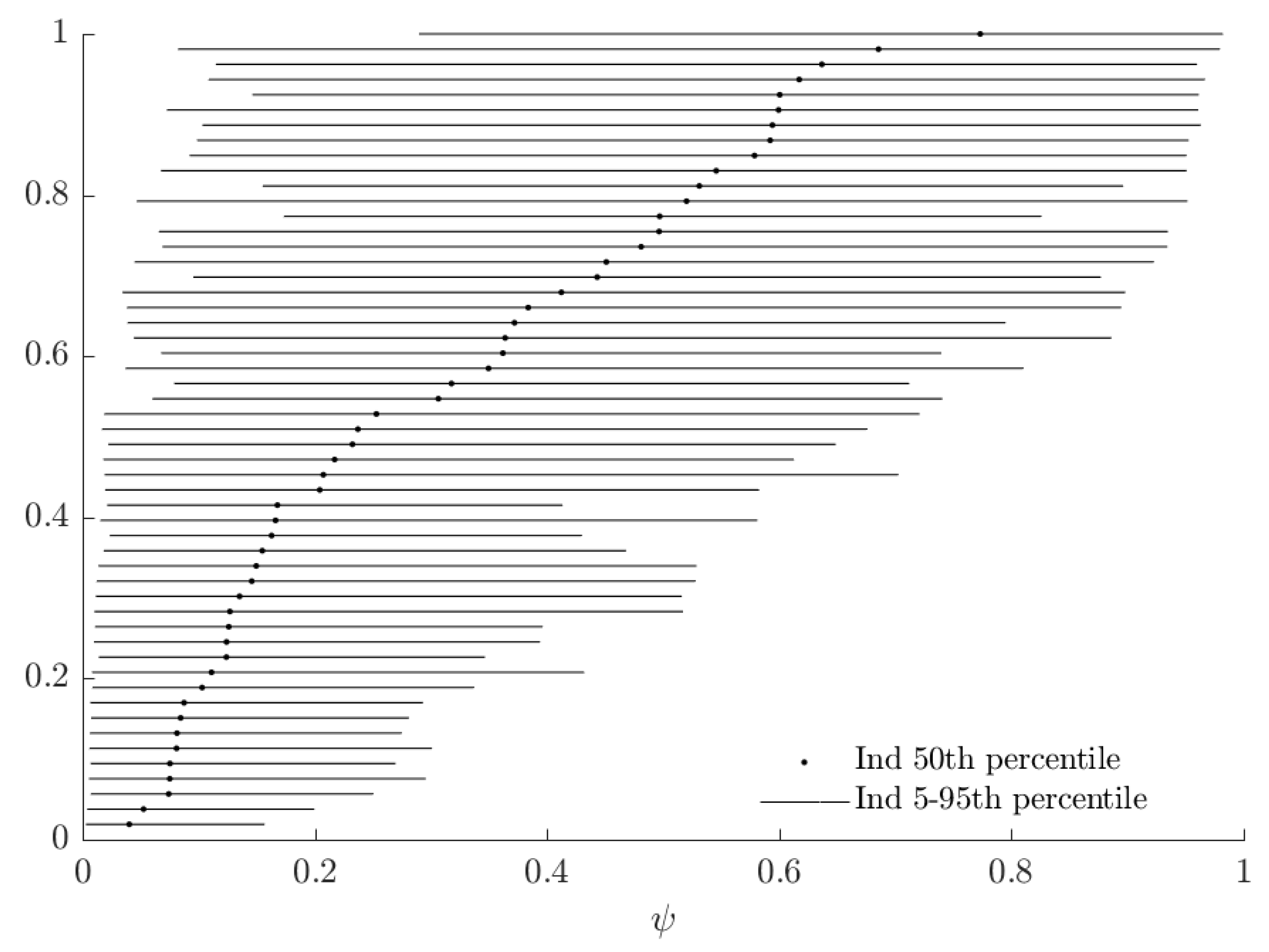
In Figure 5, the horizontal black lines show a 90% Bayesian credible region for each subject’s probability weighting parameter . The vertical red line corresponds to , and is the value for which RDEU nests EU behavior. The “mixture” part of the mixture model can be seen in this Figure as the discontinuity in the population cdf as it crosses this line, which is where the alternative model is identical to the baseline model. If a credible region is entirely to the right (left) of this line, we would assign at least 95% posterior probability to that subject’s being greater than (less than) one, and we do one of these for most subjects. This is synonymous with our estimate of the mixing probability, , being close to zero.
3.3. Rationalizable Opportunity Cost
Before analyzing the utility implications of these estimates, some consideration is prudent in deciding which estimates to use. In particular, I am seeking to evaluate the utility of subjects’ choices, assuming that the baseline model is correct. However the parameter estimates that I report in (say) Figure 4 are calculated assuming that the subject could be either of the types under consideration, and so these estimates are from the posterior distribution conditional on the data, but not on type. Instead, since I want to evaluate a subject’s utility assuming that they are in fact the baseline type: I need to condition on this information. That is, while Figure 4 reports the distribution of a transform of , where y represents the data, these estimates do not fully take into account the information provided by this assumption. Instead, I need to evaluate .15 Draws from this conditional distribution are already generated as part of the Gibbs sampling procedure (outlined in Appendix B). In short, when determining the probability that a subject takes an action, I condition estimates on the data only, but when evaluating their utility associated with these probabilities, I additionally condition on them being the baseline type.
I now turn to analyzing behavior in the utility domain. This task, while straightforward at the individual decision level, is complicated in that subjects made 500 decisions, one of which was randomly chosen for payment. For some of these decisions, subjects’ baseline and alternative decision rules could have prescribed the same action, while for other decisions, these actions could have been different. Therefore, I evaluate the expected utility of following a particular decision rule for the entire experiment, according to (8). Alternatively, ignoring any costs of time and thinking associated with participating in the experiment, the subject would be indifferent between being turned away at the beginning of the experiment, leaving with the certainty equivalent in cash, and following probabilistic decision rule for all decisions in the experiment.
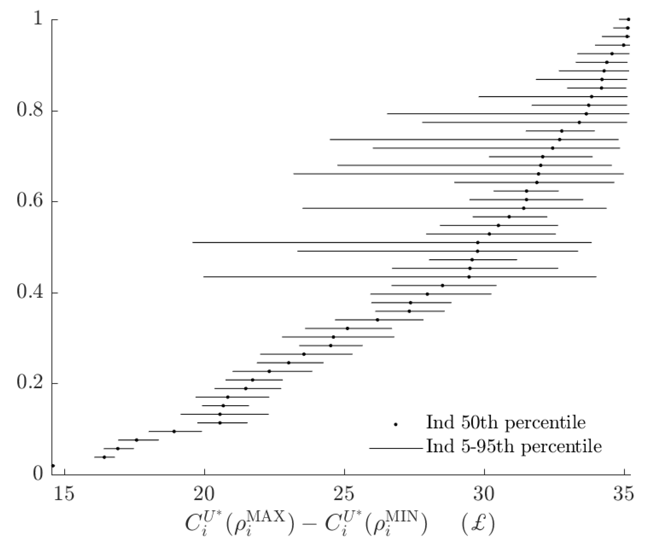
Figure 6, shows the rationalizable opportunity cost of subjects being the alternative type and making probabilistic choices. While these costs, had the BP rule prescribed many different actions to the AP rule, could be in the £15-35 range,16 in fact the BP decision rule incurs an opportunity cost of less than £4 for all subjects. That is, relative to the range of certainty equivalents that subjects could achieve, the BP rule appears to have a small total rationalizable opportunity cost.
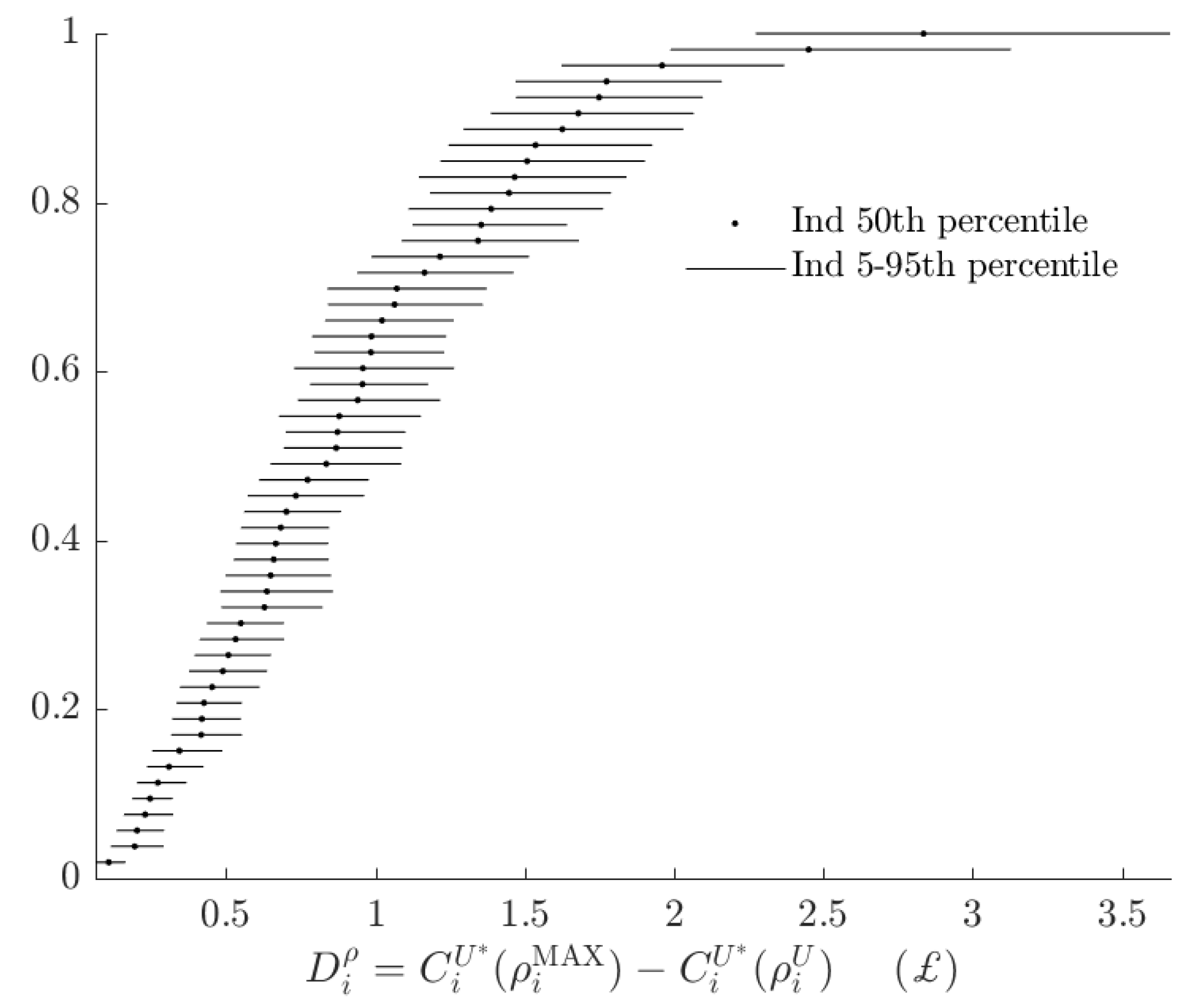
Figure 7 and Figure 8 decompose the total rationalizable opportunity cost in Figure 6 into its two components. Figure 7 shows the rationalizable opportunity cost of the alternative model, holing probabilistic choice constant. For the vast majority of subjects these costs are between £0 and £1, with most of these costs being much closer to £0 than £1. This quantity could be negative if the alternative model amplifies utility difference compared to the alternative model. Eight out of 53 subjects had posterior median estimates of this quantity strictly less than zero, however for all but one subject, the 90% Bayesian credible regions either include zero, or only cover positive values: although one could envisage parameters that make the alternative type more likely to maximize the baseline objective function than the baseline type, in practice this is unlikely.
Figure 8 shows estimates of subjects’ rationalizable opportunity cost of probabilistic choice. That is, I compute the difference between subjects’ maximum certainty equivalent, and the certainty equivalent they would achieve by following the baseline model with probabilistic choice. This is the component of the certainty equivalent shown in Figure 6 that is not “explained” by the alternative model.
These numbers are small relative to their upper bounds (Figure A1), but are similar in magnitude to total rationalizable opportunity costs (Figure 6).
In order to compare these two kinds of opportunity cost, I plot the rationalizable opportunity cost of the alternative model divided by the total rationalizable opportunity cost in Figure 9.
In this Figure, a number close to zero indicates that the alternative model does not constitute a substantial departure in utility from the baseline, when being compared to un-modeled probabilistic choice. This is the case for most subjects. In the case of this experiment, while most subjects’ choices seem to be better modeled by the alternative RDEU model, the decisions where the RDEU model is predicting different choices are likely to be ones where the stakes are low. However it is not the case that noise will always dominate total rationalizable opportunity cost for these subjects.
For example, Figure 10 shows estimates of if the subjects in this experiment were instead making a single decision between (a) a 50% chance of $1, zero otherwise, and (b) actuarily fair insurance of this event (i.e., $0.50 for sure).17 It is optimal for all EU, risk-averse subjects to purchase insurance, but the mixture model predicts that of these, some will not because of a combination of probabilistic choice and RDEU behavior. While for this decision there is still a substantial fraction of subjects for whom the alternative model does not imply a substantial rationalizable opportunity cost (those with dots to the left of the Figure), in this situation there are more subjects whose total rationalizable opportunity costs is mostly accounted for by the alternative model.
4. Conclusions
In the past decade, mixture models have greatly expanded the set of questions that we can ask of our data. Of particular interest to experimental economists is that we can take more than one theory of how people make decisions to our data at the same time. Methods developed in this paper allow us to gain additional insight from the same modeling framework. Measures of utility, such as certainty equivalents, are easily calculable from mixture models, and allow us to assess how well our models are explaining not just decisions, but also utility. As mixture models have two ways in which behavior could depart from deterministic maximization of a single objective function, comparing the rationalizable opportunity cost of each of these, and both together, is meaningful, and can identify whether behavior is not well explained by just a baseline model due to either the alternative model constituting substantial departure from the baseline in terms of utility, or something that we are not explicitly modeling: probabilistic choice.
Although I approach this problem by simply designating one of the theories under consideration in the mixture model the “baseline” model, if one is willing to take a stand that noise or the alternative model constitutes a mistake (e.g., [18], p. 29), then these rationalizable opportunity costs can also be interpreted as the costs of this mistake. If probabilistic choice is indeed noise, as treated by Alekseev et al. [7], and not un-modeled but nonetheless actual utility, then is the cost of behaving noisily. Likewise, is the utility that a subject gives up through not behaving according to the baseline model. I do not wish to take this stand here, however doing so would not change the mechanics of calculating these quantities, only their interpretation.
For the experiment studied here [8] I find that the larger contribution to total rationalizable opportunity cost for most subjects is the absolute welfare cost of probabilistic choice. Since probabilistic choice in this model does not differ between the EU and RDEU types, one can conclude that these types are economically similar in terms of utility, even if they predict different choices in many cases. As noted by Hey and Orme [9], “Perhaps we should now spend some time on thinking about the noise, rather than about even more alternatives to EU?” Furthermore, this technique could be used to design experiments where the baseline and alternative models imply both (i) substantially different actions, and (ii) substantially different utility, for the choices under consideration. For mixture models in general, this paper highlights that our conclusions about the economic significance of the theories under consideration can differ greatly depending on whether we are primarily concerned with the decisions that people make, or the utility people achieve. If one is trying to forecast actions, then modeling the former well is of course important. On the other hand if one is using mixture models to make good decisions on behalf of others, or using them to design better choice architecture, then knowing whether differences in the types’ choices imply substantially different levels of welfare is also important.
Funding
I acknowledge the support of the University of Toledo’s Summer Research Awards and Fellowships Program.
Acknowledgments
This research has been much improved by comments from Alexander Alexeev, Amanda Cook, Evan Calford, Shooshan Danagoulian, Sherry Gao, Glenn Harrison, Dale Stahl, two anonymous referees. attendees of the 2017 Economic Science Association North American meetings, attendees of the 2017 Southern Economic Association annual meetings, and attendees of the Purdue University Experimental Lunch Seminar Series, the Bowling Green State University Economics Seminar Series, the Wayne State University Economics Seminar Series, and the University of Toledo Economics Seminar Series.
Conflicts of Interest
The author declares no conflict of interest. The funders had no role in the design of the study; in the collection, analyses, or interpretation of data; in the writing of the manuscript, or in the decision to publish the results.
Abbreviations
The following abbreviations are used in this manuscript:
| AD | Alternative-Deterministic |
| AWC | Absolute Welfare Cost |
| BD | Baseline-Deterministic |
| AP | Alternative-Probabilistic |
| BP | Baseline-Probabilistic |
| CRRA | Constant relative Risk Aversion |
| EU | Expected Utility |
| RDEU | Rank Dependent Expected Utility |
| ROC | Rationalizable Opportunity Cost |
Appendix A. Additional Tables and Figures
Figure A1.
Estimates from the dichotomous mixture model. Difference in subjects’ certainty equivalents between maximizing and minimizing .
Figure A1.
Estimates from the dichotomous mixture model. Difference in subjects’ certainty equivalents between maximizing and minimizing .

The second model I estimate is a tremble model, similar to that estimated in Harrison and Rutström [1], which permits subjects to use the EU model for some decisions, and the RDEU model for others:
where () indicates that subject i uses the EU (RDEU) model for decision t. That is, a subject makes each decisions using the EU model with probability , and the remainder of them using the RDEU model.

Table A1.
Tremble model: Population-level parameter estimates from model with within-subject type trembles using Hey [8] data. Compare to Table 3 in the main part of the paper.
| r | |||
|---|---|---|---|
| Mean–Transformed | 0.404 | 21.973 | 0.927 |
| (0.03) | (1.59) | (0.03) | |
| Mean–Raw | −1.093 | 2.962 | −0.478 |
| (0.08) * | (0.07) * | (0.04) * | |
| Variance | |||
| r | 0.366 | - | - |
| (0.07) | |||
| −0.096 | 0.251 | - | |
| (0.05) * | (0.05) | ||
| 0.035 | 0.028 | 0.087 | |
| (0.03) | (0.02) | (0.02) | |
| Mean tremble probability | 0.3229 | (0.0307) |
* Indicates that a 95 percent Bayesian credible region does not include zero; Stars are suppressed because these parameters can only be positive.
Figure A2.
Tremble model: Posterior probabilities that each subject is the baseline (EU) type. Compare to Figure 3 in main part of document.
Figure A2.
Tremble model: Posterior probabilities that each subject is the baseline (EU) type. Compare to Figure 3 in main part of document.

Figure A3.
Tremble model: Estimates of (probability weighting). Compare to Figure 5 in main part of document.
Figure A3.
Tremble model: Estimates of (probability weighting). Compare to Figure 5 in main part of document.

Figure A4.
Tremble model: Probability of choosing the better lottery when the utility difference between them is 0.1. This probability is equal to . Compare to Figure 4 in main part of document.
Figure A4.
Tremble model: Probability of choosing the better lottery when the utility difference between them is 0.1. This probability is equal to . Compare to Figure 4 in main part of document.
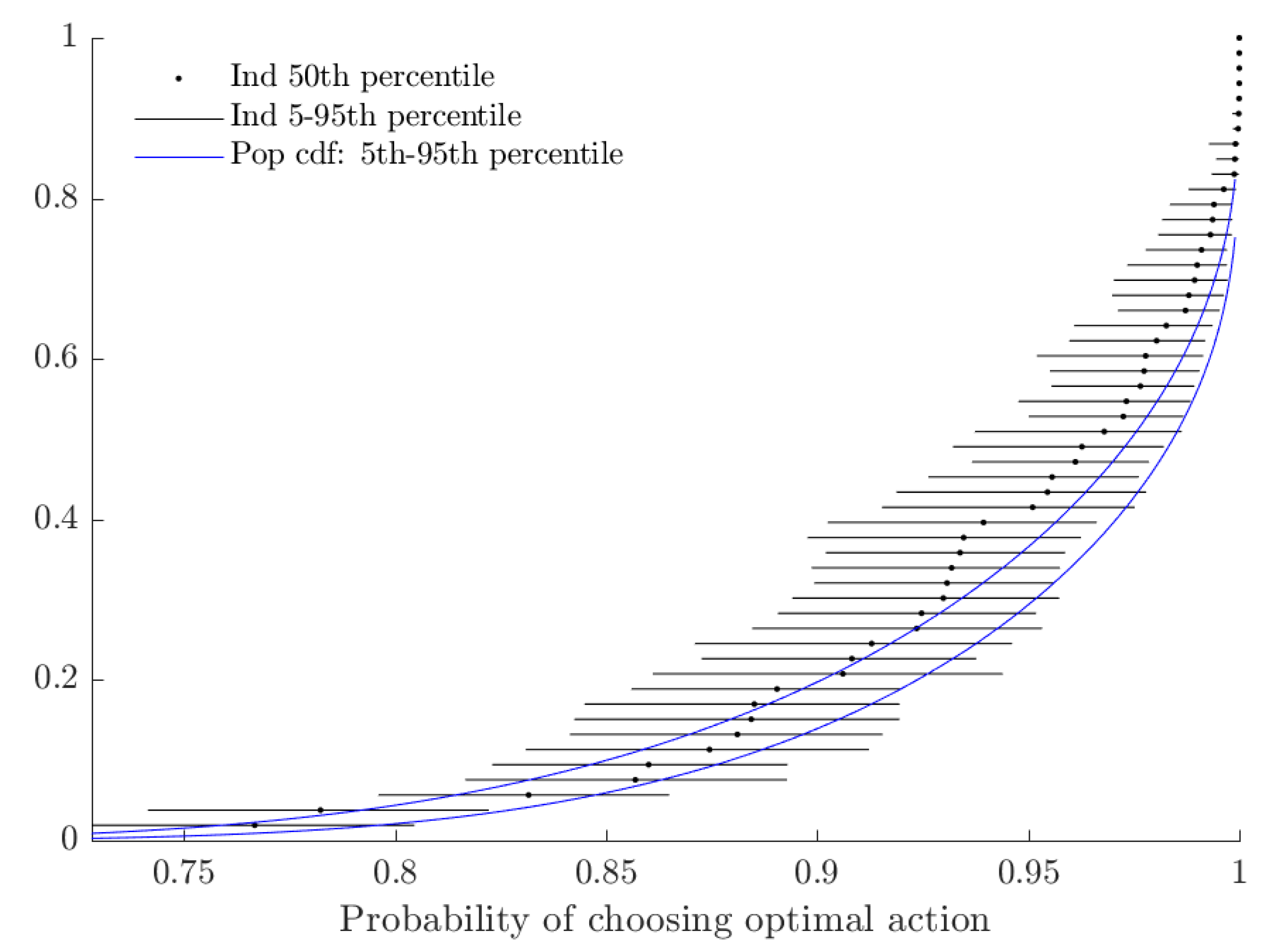
Figure A5.
Tremble model: Difference in subjects’ certainty equivalents between maximizing and minimizing . Compare to Figure A1 in main part of document.
Figure A5.
Tremble model: Difference in subjects’ certainty equivalents between maximizing and minimizing . Compare to Figure A1 in main part of document.
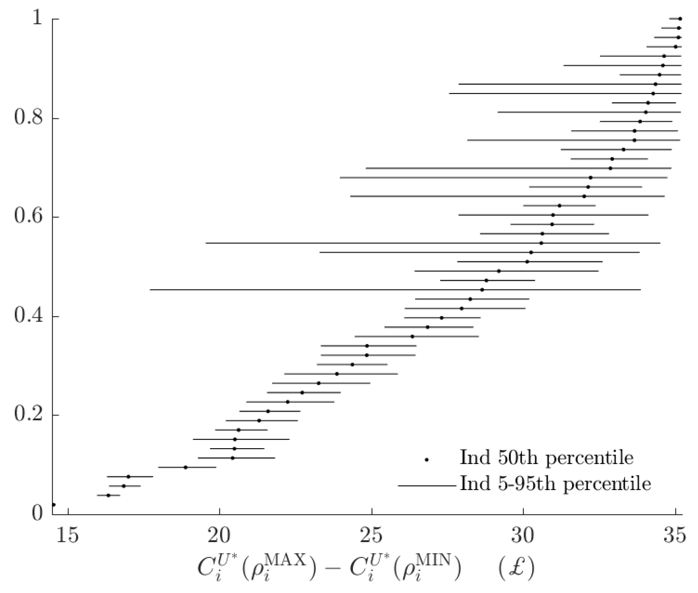
Figure A6.
Tremble model: Difference in subjects’ certainty equivalents between maximizing and implementing their estimated probabilistic decision rule. Compare to Figure 6 in main part of document.
Figure A6.
Tremble model: Difference in subjects’ certainty equivalents between maximizing and implementing their estimated probabilistic decision rule. Compare to Figure 6 in main part of document.
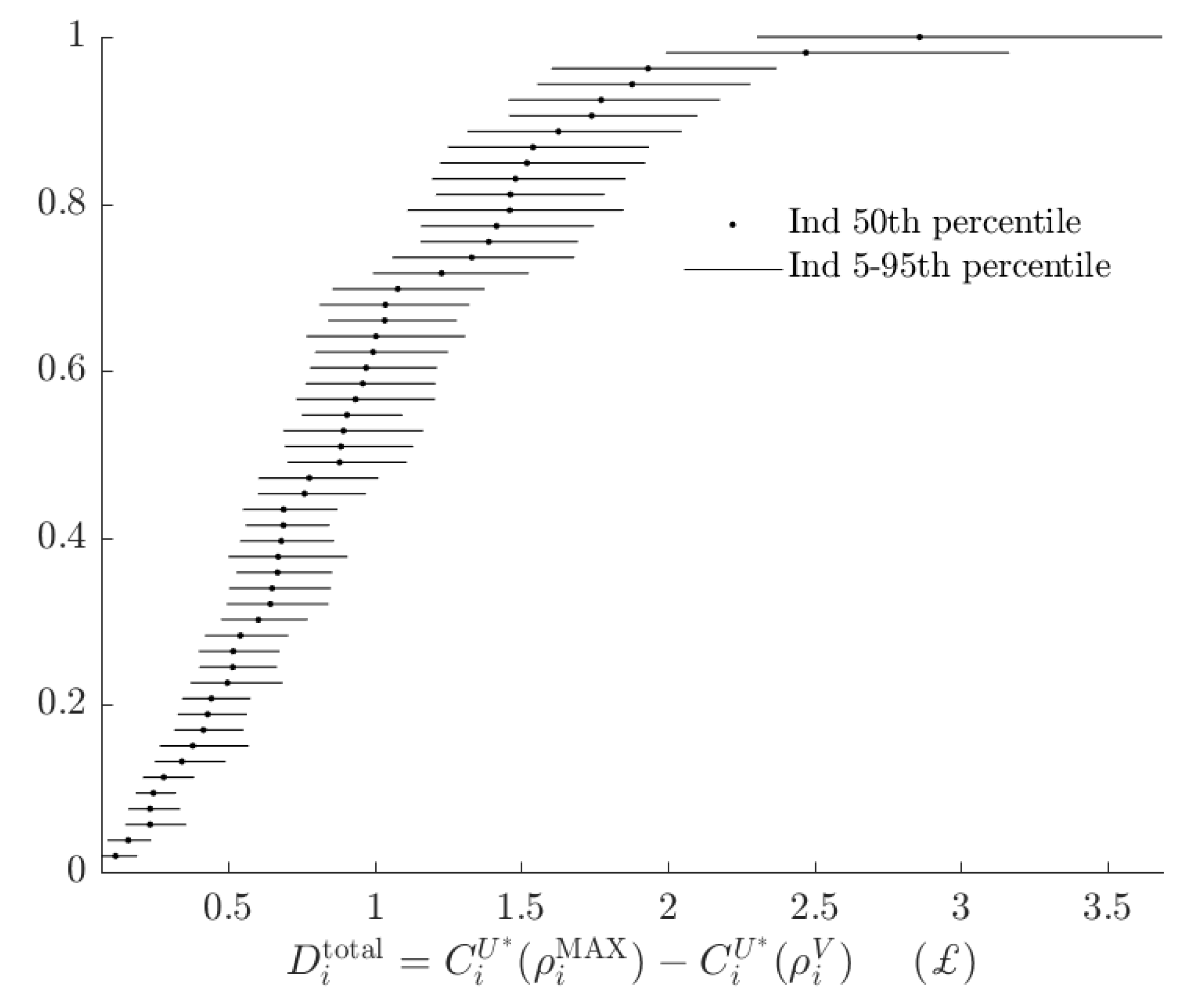
Figure A7.
Tremble model: Difference in subjects’ certainty equivalents between using the baseline and alternative models, holding the probabilistic decision rule constant. Compare to Figure 7 in main part of document.
Figure A7.
Tremble model: Difference in subjects’ certainty equivalents between using the baseline and alternative models, holding the probabilistic decision rule constant. Compare to Figure 7 in main part of document.
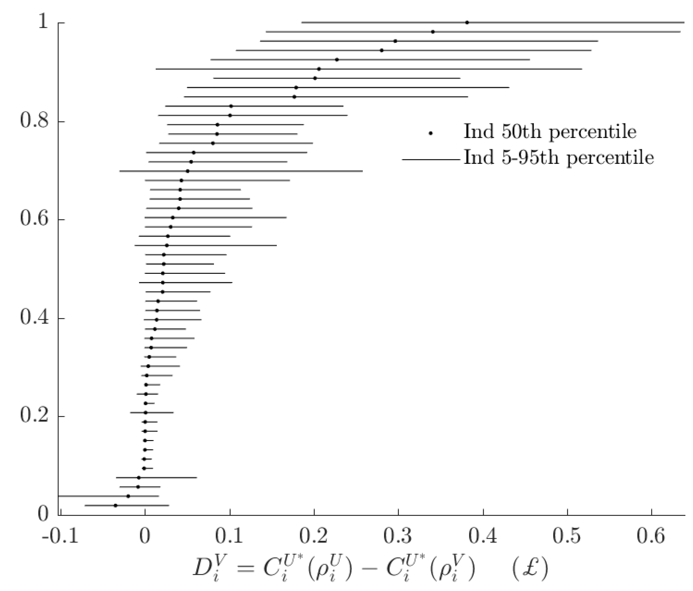
Figure A8.
Tremble model: Difference in subjects’ certainty equivalents between using deterministic and probabilistic decision rules, holding the baseline model constant.Compare to Figure 8 in main part of document.
Figure A8.
Tremble model: Difference in subjects’ certainty equivalents between using deterministic and probabilistic decision rules, holding the baseline model constant.Compare to Figure 8 in main part of document.
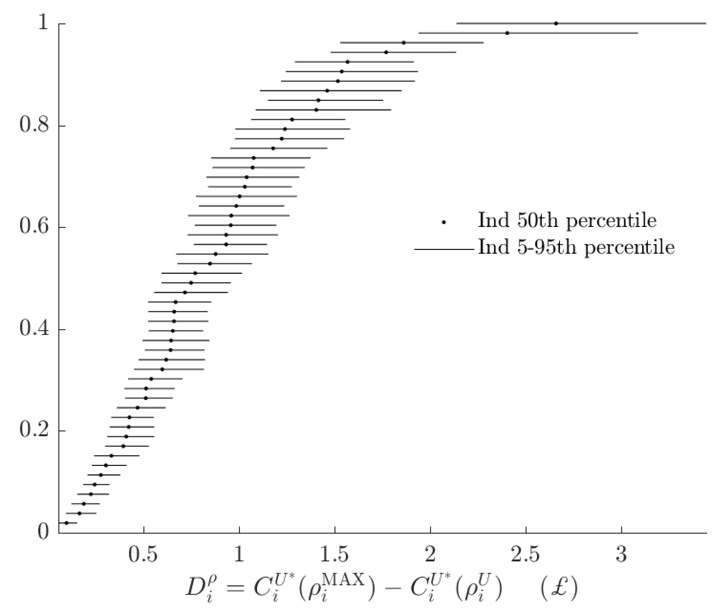
Figure A9.
Tremble model: Fraction of attributable to subjects using the alternative model. Compare to Figure 9 in main part of document.
Figure A9.
Tremble model: Fraction of attributable to subjects using the alternative model. Compare to Figure 9 in main part of document.
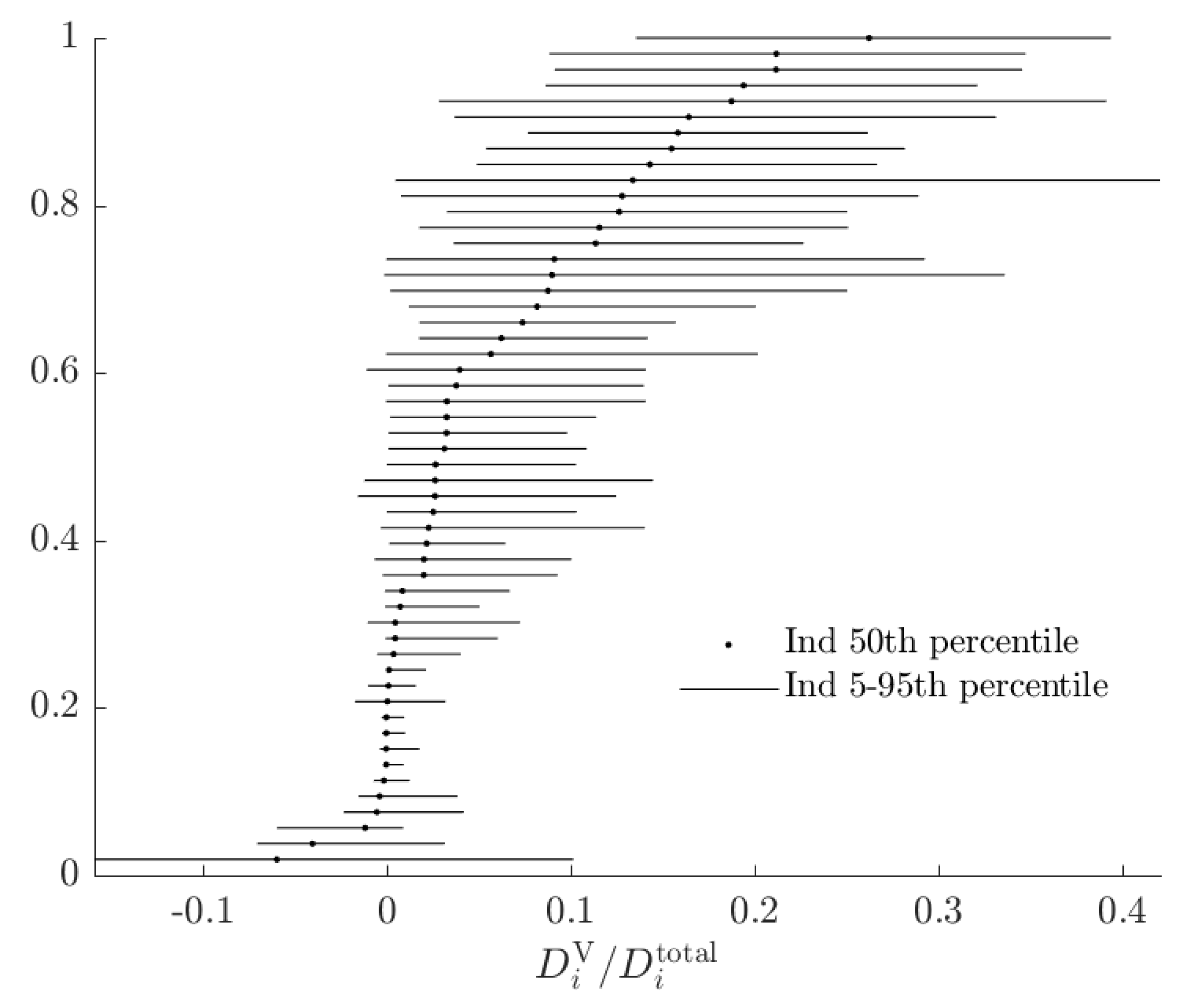
Figure A10.
Tremble model: Fraction of attributable to subjects using the alternative model, based on a decision to purchase or not purchase actuarily fair insurance against an event occurring with probability 50%.Compare to Figure 10 in main part of document.
Figure A10.
Tremble model: Fraction of attributable to subjects using the alternative model, based on a decision to purchase or not purchase actuarily fair insurance against an event occurring with probability 50%.Compare to Figure 10 in main part of document.
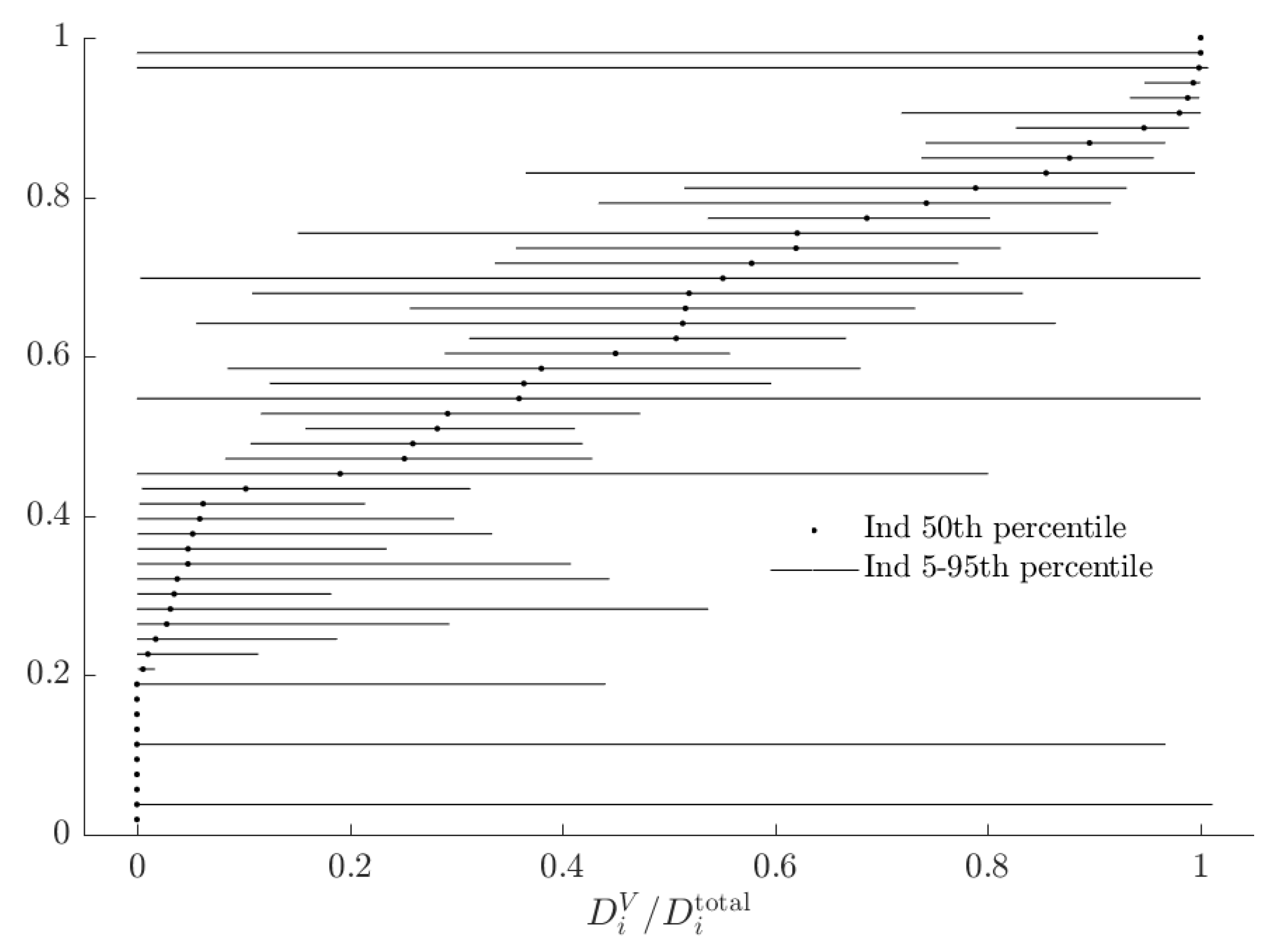
Table A2.
Posterior means of mixture model assuming that probabilistic choice () is constant within a type, and that subjects have a common type tremble ().This specification is identical to Conte et al. [2], except that here I assume that the joint distribution of is identical between types, whereas Conte et al. [2] assume that it is type-specific.
| r | ||
|---|---|---|
| Mean–Transformed | 0.421 | 1.069 |
| (0.03) | (0.18) | |
| Mean–Raw | −1.043 | −0.317 |
| (0.08) * | (0.20) * | |
| Variance | ||
| r | 0.349 | - |
| (0.07) | ||
| 0.010 | 0.116 | |
| (0.09) | (0.05) | |
| 0.5224 | (0.0684) | |
| 0.0376 | (0.0013) | |
| 0.0481 | (0.0017) | |
| (decision tremble) | 0.0069 | (0.0009) |
* Indicates that a 95 percent Bayesian credible region does not include zero; a Stars are suppressed because these parameters can only be positive.
Appendix B. Notes on Bayesian Estimator
I make the following assumptions about the data-generating process:
- At the individual level, subjects’ behavior is described by one of two models, indexed . Each model specifies a likelihood function mapping individual parameters into a probability distribution over actions . These models are:where () if and only if subject i chose ( ) in lottery pair t.
- Subjects’ behavior is independent:
- Individual-level parameters are iid multivariate normal draws:
- Subjects are type 1 () with probability , and type 2 otherwise.
I simulate the posterior distribution . To this end, I augment the data with the individual-level parameters and to get the joint posterior distribution of :
where is subject i’s likelihood conditional on having parameters and being type . The final equality assumes that for the prior distribution, is independent of .
Using Gibbs sampling, we can draw from this distribution if we can draw from its conditionals. Broadly, this will be done in four steps (excluding an initialization):
- 0.
- Initialization: Choose initial values
- 1.
- Draw from . Inspection of (A9) yields that:Using a Normal-Inverse-Wishart prior , with independent of in the prior distribution, then:where . See (Ex. 12.1, Koop et al. [19]) for a more general derivation of this result. We can therefore draw from as follows:
- l.1
- Draw
- l.2
- Draw
I choose the following parameters for this part of the prior distribution: - 2.
- Draw for each model . The relevant component of (A9) is:As is non-standard, I use the Metropolis-Hastings algorithm to complete this step.
- 3.
- Draw , and update to be the one from above specific to this draw. The relevant component of (A9) is:Note that the simulated values of (A18) can be used to assign posterior probabilities to individual subjects being each type.
- 4.
- Draw . From (A9):If we assume a Dirichlet prior:then:Here I choose prior parameters , which corresponds to a uniform prior over the fraction of subjects who are the EU type.
- 5.
- Go back to step 1.
References
- Harrison, G.W.; Rutström, E.E. Expected utility theory and prospect theory: One wedding and a decent funeral. Exp. Econ. 2009, 12, 133–158. [Google Scholar] [CrossRef]
- Conte, A.; Hey, J.D.; Moffatt, P.G. Mixture models of choice under risk. J. Econ. 2011, 162, 79–88. [Google Scholar] [CrossRef] [Green Version]
- Harrison, G.W.; Lau, M.I.; Rutström, E.E. Individual discount rates and smoking: Evidence from a field experiment in Denmark. J. Health Econ. 2010, 29, 708–717. [Google Scholar] [CrossRef] [PubMed]
- Bland, J.R. How many games are we playing? An experimental analysis of choice bracketing in games. J. Behav. Exp. Econ. 2019, 80, 80–91. [Google Scholar] [CrossRef]
- Quiggin, J. A theory of anticipated utility. J. Econ. Behav. Org. 1982, 3, 323–343. [Google Scholar] [CrossRef]
- Harrison, G.W. Theory and Misbehavior of First-Price Auctions. Am. Econ. Rev. 1989, 79, 749–762. [Google Scholar]
- Alekseev, A.; Harrison, G.W.; Lau, M.; Ross, D. Deciphering the Noise: The Welfare Costs of Noisy Behavior. Available online: https://research.cbs.dk/en/publications/deciphering-the-noise-the-welfare-costs-of-noisy-behavior (accessed on 17 April 2018).
- Hey, J.D. Does repetition improve consistency? Exp. Econ. 2001, 4, 5–54. [Google Scholar] [CrossRef]
- Hey, J.D.; Orme, C. Investigating generalizations of expected utility theory using experimental data. Econ. J. Econ. Soc. 1994, 62, 1291–1326. [Google Scholar] [CrossRef]
- Rabin, M.; Weizsäcker, G. Narrow bracketing and dominated choices. Am. Econ. Rev. 2009, 99, 1508–1543. [Google Scholar] [CrossRef] [Green Version]
- Harrison, G.W.; Martínez-Correa, J.; Swarthout, J.T. Reduction of compound lotteries with objective probabilities: Theory and evidence. J. Econ. Behav. Org. 2015, 119, 32–55. [Google Scholar] [CrossRef] [Green Version]
- Bland, J.R.; Rosokha, Y. Learning Under Uncertainty with Multiple Priors: Experimental Investigation. 2019. Available online: https://papers.ssrn.com/sol3/papers.cfm?abstract_id=3419020 (accessed on 12 July 2019).
- Machina, M.J. Stochastic Choice Functions Generated From Deterministic Preferences Over Lotteries. Econ. J. 1985, 95, 575–594. [Google Scholar] [CrossRef]
- Elabed, G.; Carter, M.R. Compound-risk aversion, ambiguity and the willingness to pay for microinsurance. J. Econ. Behav. Org. 2015, 118, 150–166. [Google Scholar] [CrossRef]
- Andreoni, J.; Sprenger, C. Uncertainty Equivalents: Testing the Limits of the Independence Axiom; Technical Report; National Bureau of Economic Research: Cambridge, MA, USA, 2011. [Google Scholar]
- Agranov, M.; Ortoleva, P. Stochastic choice and preferences for randomization. J. Political Econ. 2017, 125, 40–68. [Google Scholar] [CrossRef] [Green Version]
- Moffatt, P.G. Stochastic Choice and the Allocation of Cognitive Effort. Exp. Econ. 2005, 8, 369–388. [Google Scholar] [CrossRef]
- Thaler, R.H. Misbehaving: The Making of Behavioral Economics; WW Norton & Company: New York, NY, USA, 2015. [Google Scholar]
- Koop, G.; Poirier, D.J.; Tobias, J.L. Bayesian Econometric Methods; Cambridge University Press: Cambridge, UK, 2007. [Google Scholar]
| 1. | |
| 2. | Stochastic choice rules are also an econometric necessity when using likelihood-based techniques: if a subject makes just one decision that does not maximize her objective function, then without a probabilistic choice rule, the likelihood function (before taking logs) is zero everywhere, and hence cannot be maximized. |
| 3. | Such a mis-classification could be reasonably likely if the alternative model generalizes the baseline. For example, consider a simple mixture model that assumes subjects either maximize expected value (the baseline type), or maximize a constant relative risk aversion utility function (the alternative type). It is likely in this situation that some expected value-maximizers will be classified as expected utility-maximizers. |
| 4. | Note that while it may at first seem reasonable that could only be positive, this is not necessarily the case. This is because, for the choice set under consideration, it is possible that the alternative objective function exaggerates the utility differences. For example, a risk-neutral subject faced with choosing between a 25% chance of winning $2, or zero otherwise, and $1 for sure, would evaluate this utility difference as . Alternatively, if a subject weighs probability with weighting function , but was otherwise risk-neutral, then they will perceive this difference as . Holding the level of noise constant in the probabilistic choice rule, the subject who weighs probability is more likely to choose the lottery that maximizes U, even though they are not seeking to maximize it. |
| 5. | Alekseev et al. [7] define this quantity more generally as “the monetary welfare that the agent would be allowed to give up for exactly of her choices to be rationalized by the model, given noise ” ( in the insurance example). Within this framework, I set , and hence compute the monetary welfare that the agent would be allowed to give up for all of her choices to be rationalized by the baseline model. |
| 6. | e.g., for an expected utility model, simply normalizing utility over money to be between 0 and 1 means that the expected utility is the uncertainty equivalent. |
| 7. | In the experiment, subjects were presented these prizes as -£25, £25, £75, and £125, plus a £25 show-up fee. I maintain the assumption of Conte et al. [2] that subjects integrate the show-up fee with the lottery prize, so I will proceed in terms of the integrated payoffs only. |
| 8. | Here I assume for simplicity that if i is indifferent, she will choose . |
| 9. | As this is a CRRA utility function, this normalization is equivalent to multiplying the utility function by (a constant at the subject level), and hence dos not affect estimates of . It will affect estimate of the variance of decision errors (i.e., they will be inflated by ). |
| 10. | The lower bound of ensures that the probability weighting function is always increasing in p. |
| 11. | See Bland and Rosokha [12] for an exception. |
| 12. | In Appendix A I show the results of a model that assumes subjects tremble between the two preference functionals, rather than using one for the entire experiment. This specification is similar to the specification for mixing in Harrison and Rutström [1]. While the mixing probability is substantially larger in this model, the other results for this model are quantitatively similar to the results discussed in the main part of this paper. |
| 13. | Conte et al. [2] estimate this number to be 20%. I suspect this difference is due to several differences in the econometric specification outlined above. |
| 14. | For reference, the average difference in expected values for this experiment was £15.19. As I divide prizes by the maximum payout, this corresponds to a difference of units of normalized utility difference for a risk-neutral subject. |
| 15. | Alternatively, from a maximum likelihood perspective, suppose that I estimated a subjects’ parameters on the individual level to be , and then estimated a restricted model that only permitted EU types, producing estimates . I need to use when determining what a subject would do conditional on being the alternative type, but I need to use when evaluating the certainty equivalent associated with doing this, because I need the best possible estimate of their parameters conditional on being the baseline type. |
| 16. | See Figure A1 in Appendix A for these estimates. |
| 17. | Because I use a constant relative risk aversion specification, the stakes do not change these estimates. |
Figure 1.
Certainty equivalents of behaving according to Expected Utility and Rank Dependent Expected Utility models when purchasing insurance. Certainty equivalents are evaluated assuming that preferences are actually represented by the EU model.
Figure 1.
Certainty equivalents of behaving according to Expected Utility and Rank Dependent Expected Utility models when purchasing insurance. Certainty equivalents are evaluated assuming that preferences are actually represented by the EU model.
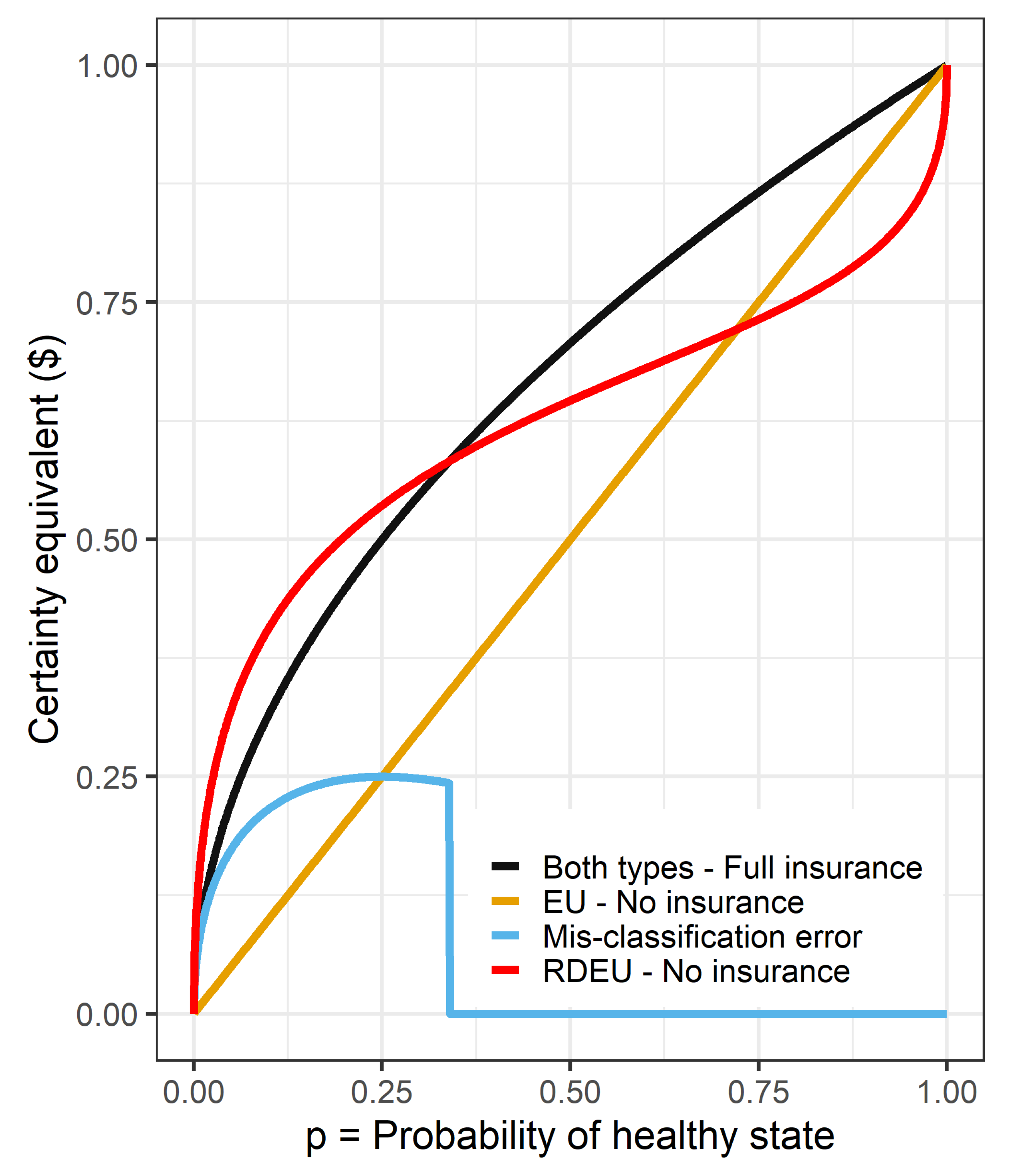
Figure 2.
Certainty equivalents of following EU and RDEU decision rules with logit choice. Probability of healthy state is .
Figure 2.
Certainty equivalents of following EU and RDEU decision rules with logit choice. Probability of healthy state is .
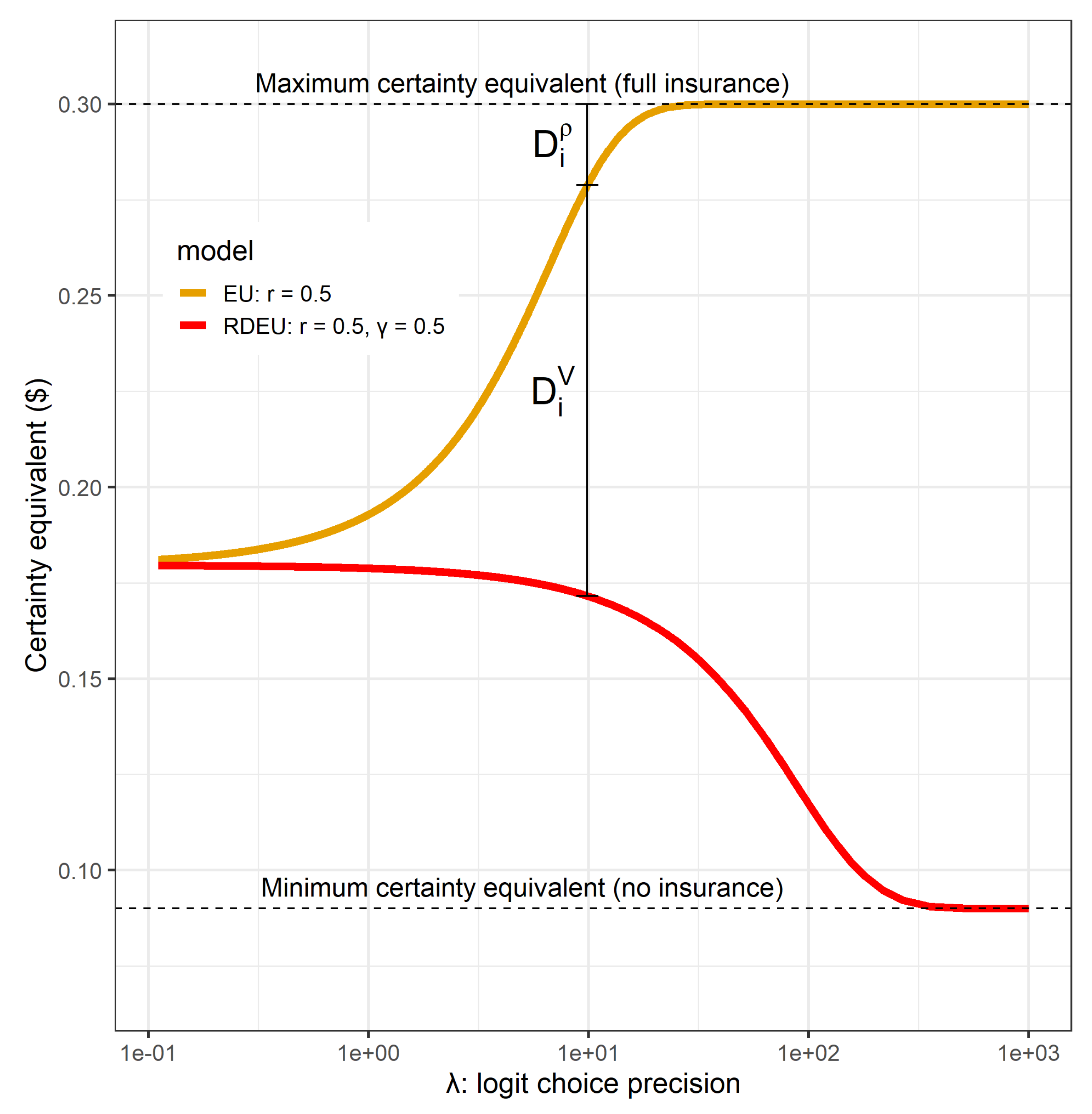
Figure 3.
Posterior probabilities that each subject is the baseline (EU) type.

Figure 4.
Probability of choosing the better lottery when the utility difference between them is 0.1. This probability is equal to .
Figure 4.
Probability of choosing the better lottery when the utility difference between them is 0.1. This probability is equal to .
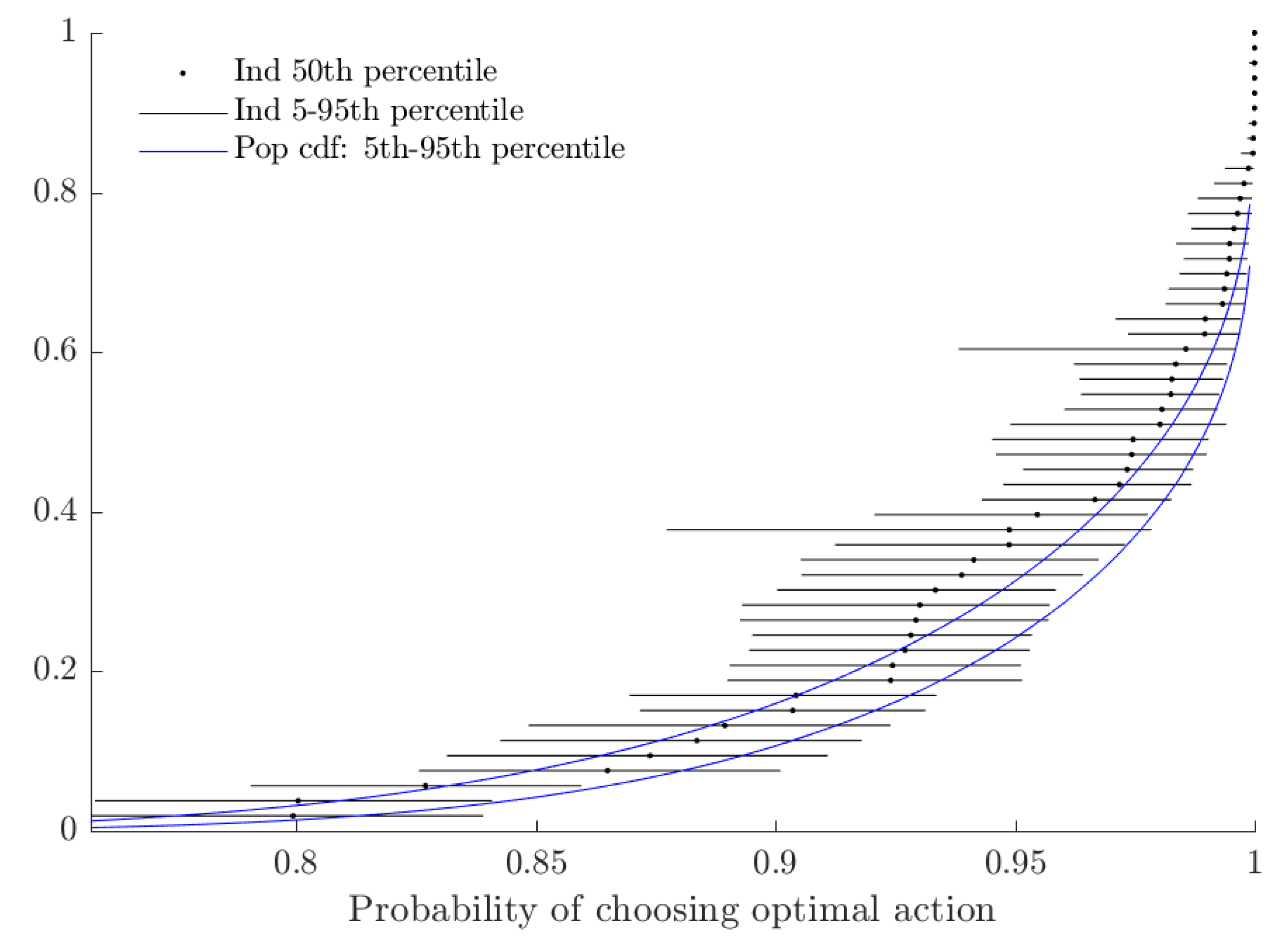
Figure 5.
Estimates of (probability weighting).
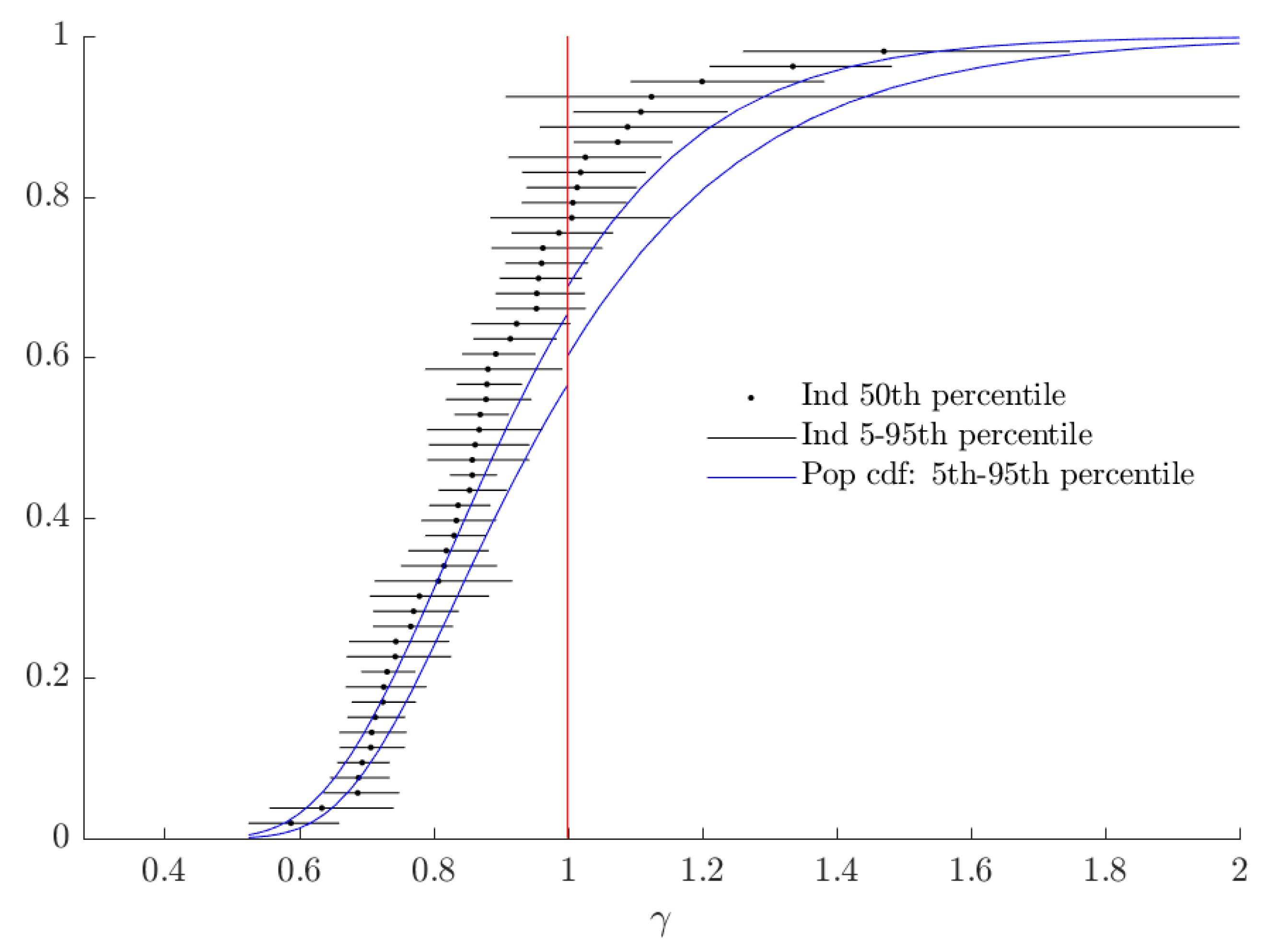
Figure 6.
Difference in subjects’ certainty equivalents between maximizing and implementing their estimated probabilistic decision rule.
Figure 6.
Difference in subjects’ certainty equivalents between maximizing and implementing their estimated probabilistic decision rule.
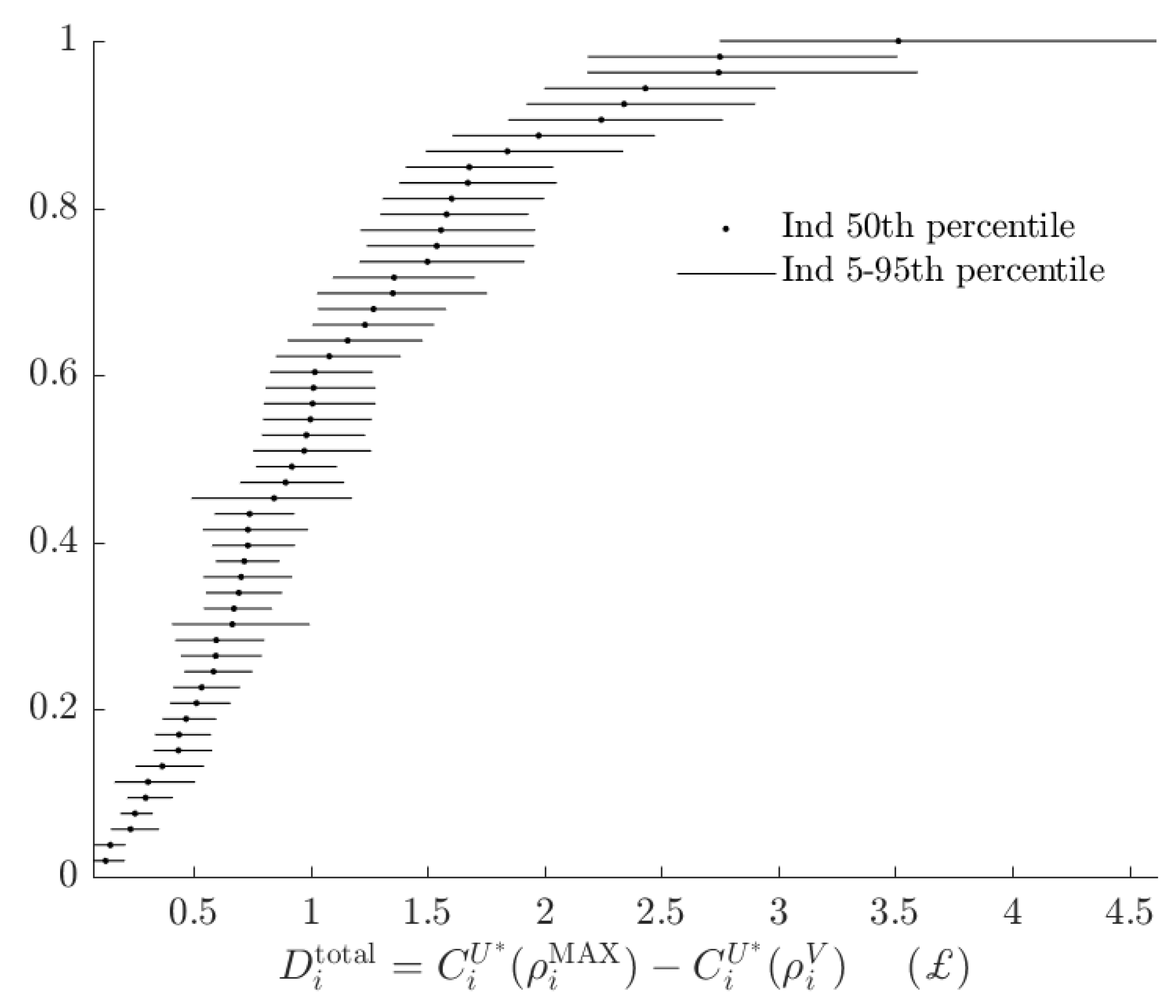
Figure 7.
Difference in subjects’ certainty equivalents between using the baseline and alternative models, holding the probabilistic decision rule constant.
Figure 7.
Difference in subjects’ certainty equivalents between using the baseline and alternative models, holding the probabilistic decision rule constant.
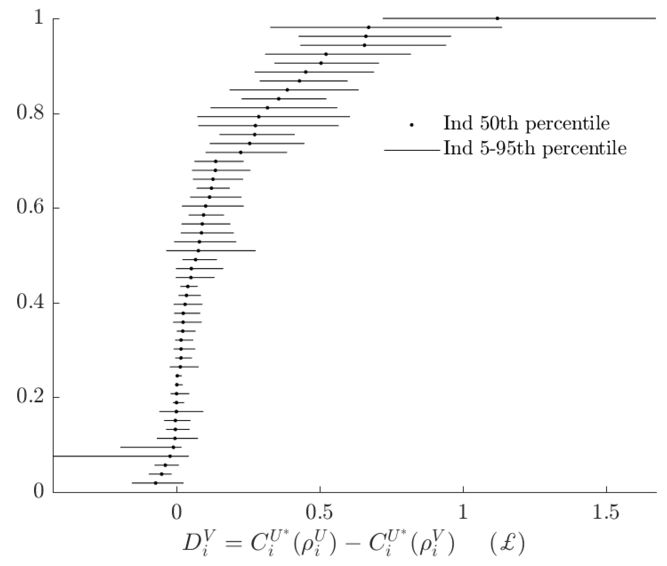
Figure 8.
Difference in subjects’ certainty equivalents between using deterministic and probabilistic decision rules, holding the baseline model constant.
Figure 8.
Difference in subjects’ certainty equivalents between using deterministic and probabilistic decision rules, holding the baseline model constant.

Figure 9.
Fraction of attributable to subjects using the alternative model, based on the 500 binary choices in Hey [8].
Figure 9.
Fraction of attributable to subjects using the alternative model, based on the 500 binary choices in Hey [8].
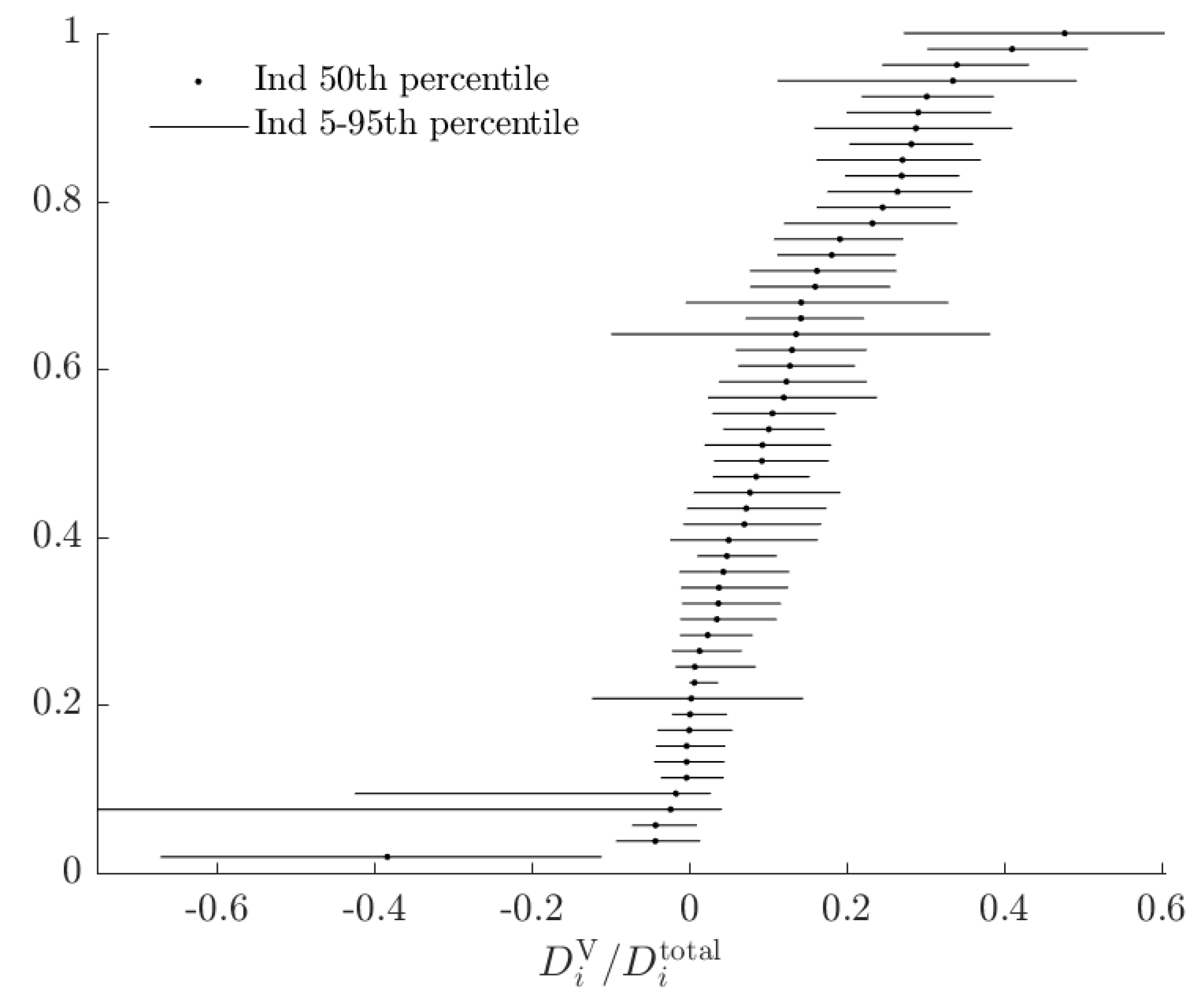
Figure 10.
Fraction of attributable to subjects using the alternative model, based on a decision to purchase or not purchase actuarily fair insurance against an event occurring with probability 50%.
Figure 10.
Fraction of attributable to subjects using the alternative model, based on a decision to purchase or not purchase actuarily fair insurance against an event occurring with probability 50%.
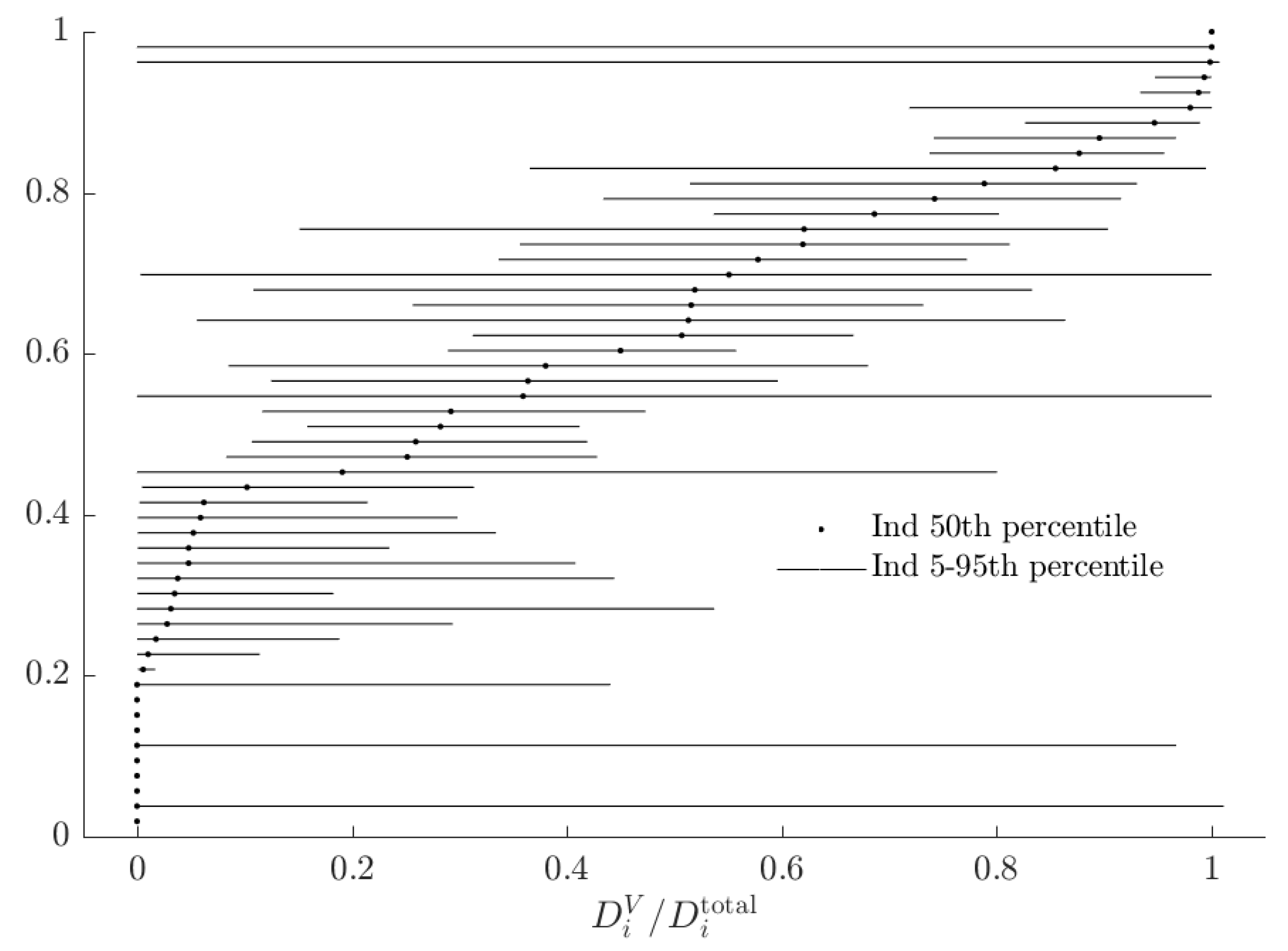
Table 1.
Alternative theories studied in some experiments, suggested classification into a baseline and behavioral type, and assumed idiosyncratic errors.
Table 1.
Alternative theories studied in some experiments, suggested classification into a baseline and behavioral type, and assumed idiosyncratic errors.
| Paper | Baseline Type | Alternative Type | Errors |
|---|---|---|---|
| Harrison [6] | Risk neutrality | Risk aversion | - |
| Hey and Orme [9] | Expected utility | Any or all of the remaining 10 models considered | power |
| Harrison and Rutström [1] | Expected utility | Prospect Theory | Logistic |
| Rabin and Weizsäcker [10] | Broad bracketing | Narrow bracketing | Logistic |
| Harrison et al. [3] | Exponential discounting | Hyperbolic discounting | Logistic |
| Conte et al. [2] | Expected utility | Rank dependent expected utility | Probit + trembles |
| Harrison et al. [11] | Reduces compound lotteries | Treats simple and compound lotteries differently | Logistic |
| Bland [4] | Broad bracketing | Narrow bracketing | Logistic |
| Bland and Rosokha [12] | Bayesian updating | Ambiguity aversion | Logistic |
Table 2.
A classification of behavior based on objective functional and noise.
| Probabilistic | Deterministic | |
|---|---|---|
| Baseline | ||
| Alternative |
Table 3.
Population-level parameter estimates from mixture model using Hey [8] data.
Table 3.
Population-level parameter estimates from mixture model using Hey [8] data.
| r | |||
|---|---|---|---|
| Mean–Transformed | 0.426 | 23.572 | 0.931 |
| (0.03) | (1.73) | (0.03) | |
| Mean–Raw | −1.009 | 3.032 | −0.493 |
| (0.07) * | (0.07) * | (0.05) * | |
| Variance | |||
| r | 0.306 | - | - |
| (0.06) | |||
| −0.094 | 0.250 | - | |
| (0.04) * | (0.05) | ||
| 0.046 | −0.001 | 0.127 | |
| (0.03) | (0.03) | (0.03) | |
| 0.0329 | (0.0309) |
* Indicates that a 95 percent Bayesian credible region does not include zero; Stars are suppressed because these parameters can only be positive.
© 2019 by the author. Licensee MDPI, Basel, Switzerland. This article is an open access article distributed under the terms and conditions of the Creative Commons Attribution (CC BY) license (http://creativecommons.org/licenses/by/4.0/).
Share and Cite
MDPI and ACS Style
Bland, J.R. Measuring and Comparing Two Kinds of Rationalizable Opportunity Cost in Mixture Models. Games 2020, 11, 1. https://doi.org/10.3390/g11010001
AMA Style
Bland JR. Measuring and Comparing Two Kinds of Rationalizable Opportunity Cost in Mixture Models. Games. 2020; 11(1):1. https://doi.org/10.3390/g11010001
Chicago/Turabian StyleBland, James R. 2020. "Measuring and Comparing Two Kinds of Rationalizable Opportunity Cost in Mixture Models" Games 11, no. 1: 1. https://doi.org/10.3390/g11010001
Note that from the first issue of 2016, this journal uses article numbers instead of page numbers. See further details here.