Behavior in Strategic Settings: Evidence from a Million Rock-Paper-Scissors Games

 , ,
, ,
Abstract
1. Data: Roshambull
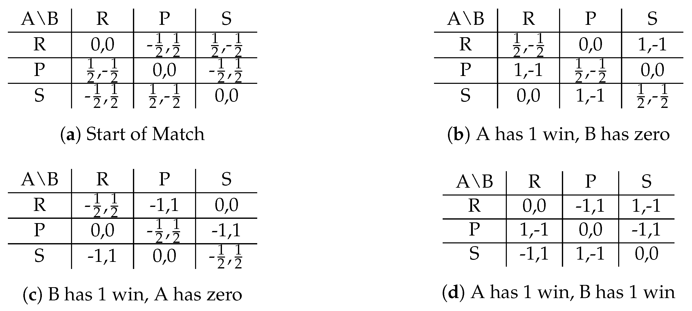
2. Model
3. Players Respond to Information
4. Level-k Behavior
4.1. Reduced-Form Evidence for Level-k Play
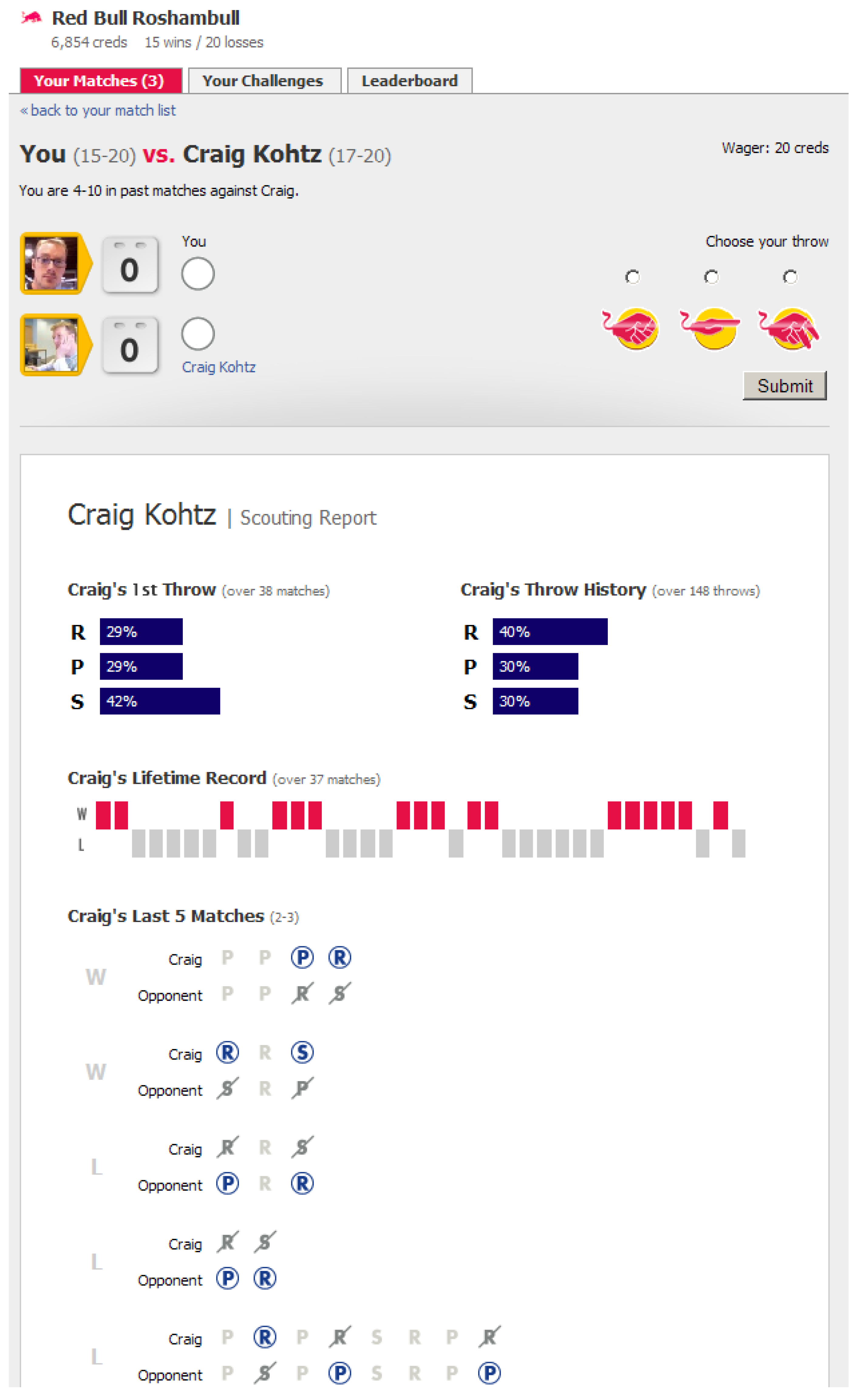
Multinomial Logit
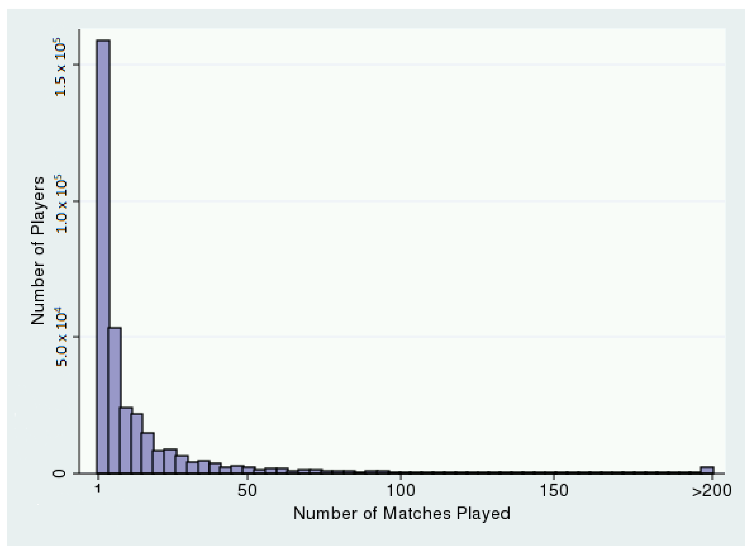
4.2. Maximum Likelihood Estimation of a Structural Model of Level-k Thinking
4.3. Cognitive Hierarchy
- randomizes according to the opponent’s historical distribution 79.92% of the time
- chooses (randomly between) the throw(s) that maximize expected payoff against the player’s own historical distribution 20.08% of the time
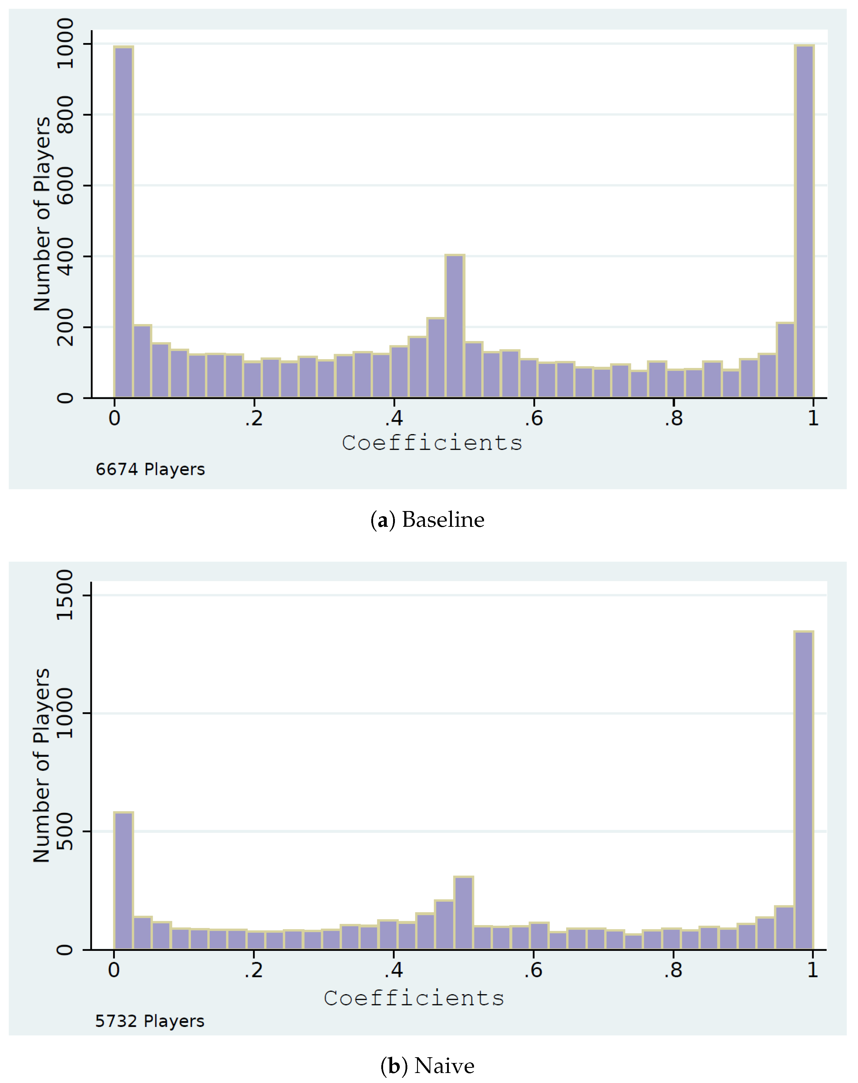
4.4. Naive Level-k Strategies
4.5. Comparisons
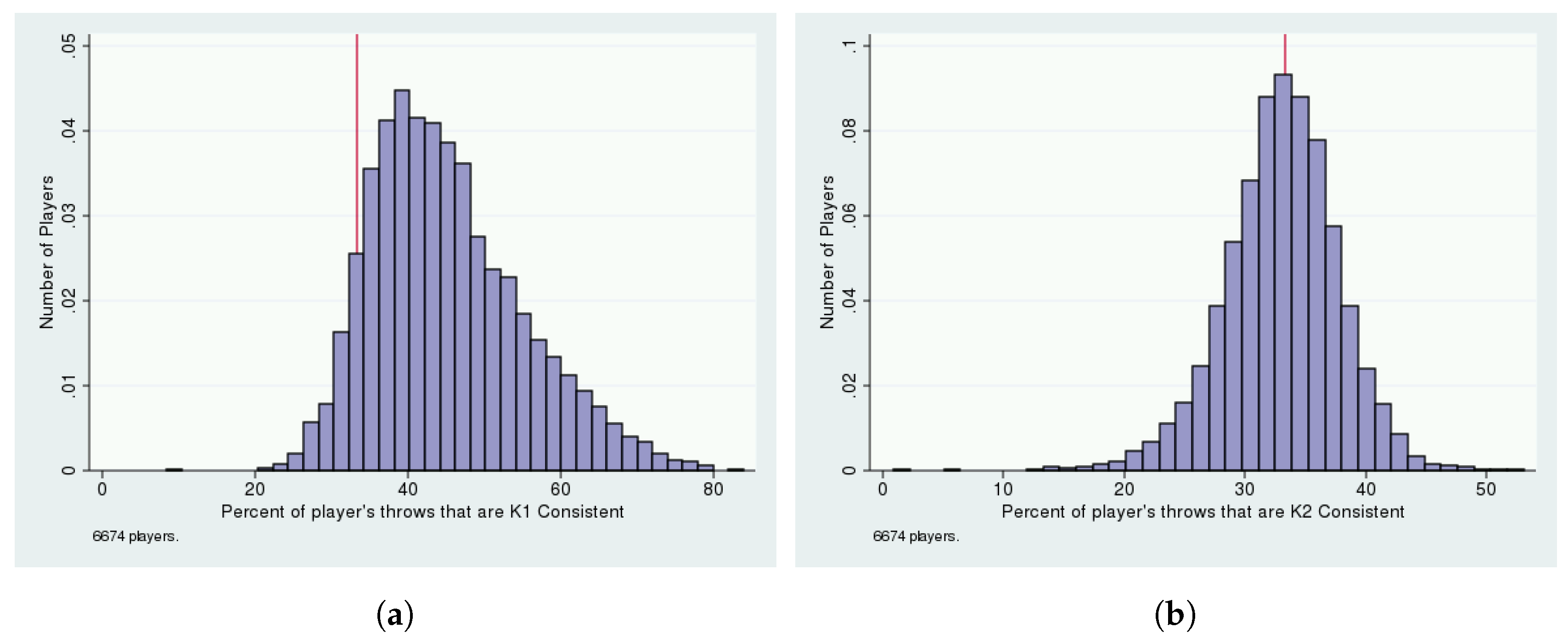
4.6. When Are Players’ Throws Consistent with ?
5. (Non-Equilibrium) Quantal Response
6. Likelihood Comparison
7. Conclusions
Author Contributions
Funding
Conflicts of Interest
Appendix A. Behavior in Strategic Settings: Evidence from a Million Rock-Paper-Scissors Games
Appendix A.1. Proof of Proposition 1

Appendix A.2. Additional Tables

| Opp’s Historical % | Throws (%) | N | ||
|---|---|---|---|---|
| Paper | Rock | Scissors | ||
| 0%–25% | 38.88 | 38.26 | 22.87 | 904,003 |
| 25%–30% | 36.93 | 39.04 | 24.03 | 568,683 |
| 30%–% | 35.95 | 37.56 | 26.49 | 475,438 |
| %–37% | 35.23 | 34.39 | 30.37 | 888,846 |
| 37%–42% | 32.86 | 29.76 | 37.39 | 671,106 |
| 42%–100% | 29.91 | 28.03 | 42.06 | 1,173,439 |
| Opp’s Historical % | Throws (%) | N | ||
|---|---|---|---|---|
| Paper | Rock | Scissors | ||
| 0%–25% | 39.61 | 28.05 | 32.34 | 1,308,484 |
| 25%–30% | 37.96 | 28.07 | 33.98 | 730,391 |
| 30%–% | 35.92 | 29.67 | 34.41 | 546,698 |
| %–37% | 32.85 | 34.29 | 32.86 | 825,972 |
| 37%–42% | 28.77 | 40.99 | 30.24 | 513,185 |
| 42%–100% | 27.24 | 46.64 | 26.12 | 756,785 |
| Covariate | Dependent Var: Dummy for Throwing Rock | ||
|---|---|---|---|
| (1) | (2) | (3) | |
| Opp’s Fraction Paper (first) | −0.0403 *** | −0.0718 *** | −0.0952 *** |
| (0.0021) | (0.0056) | (0.0087) | |
| Opp’s Fraction Scissors (first) | 0.2375 *** | 0.1552 *** | 0.1377 *** |
| (0.0022) | (0.0060) | (0.0094) | |
| Opp’s Fraction Paper (all) | 0.0022 | 0.0249 ** | 0.0032 |
| (0.0032) | (0.0088) | (0.0138) | |
| Opp’s Fraction Scissors (all) | 0.0403 *** | 0.0238 * | −0.0187 |
| (0.0033) | (0.0093) | (0.0146) | |
| Opp’s Paper Lag | 0.0043 *** | −0.0016 | −0.0043 * |
| (0.0007) | (0.0015) | (0.0019) | |
| Opp’s Scissors Lag | 0.0142 *** | 0.0052 ** | −0.0018 |
| (0.0008) | (0.0016) | (0.0020) | |
| Own Fraction Paper (first) | −0.0657 *** | 0.0290 *** | −0.1092 *** |
| (0.0020) | (0.0073) | (0.0176) | |
| Own Fraction Scissors (first) | −0.0816 *** | 0.0013 | −0.3216 *** |
| (0.0021) | (0.0076) | (0.0180) | |
| Own Fraction Paper (all) | −0.0184 *** | −0.0551 *** | −0.1408 *** |
| (0.0030) | (0.0113) | (0.0244) | |
| Own Fraction Scissors (all) | −0.0097 ** | −0.0781 *** | −0.0691 ** |
| (0.0032) | (0.0119) | (0.0253) | |
| Own Paper Lag | −0.0015 * | 0.0121 *** | 0.0046 * |
| (0.0007) | (0.0015) | (0.0019) | |
| Own Scissors Lag | 0.0031 *** | 0.0094 *** | −0.0059 ** |
| (0.0008) | (0.0016) | (0.0019) | |
| Constant | 0.3423 *** | −0.0190 *** | 0.0001 |
| (0.0007) | (0.0014) | (0.0018) | |
| 0.0184 | |||
| N | 4,433,260 | ||
| Covariate | Dependent Var: Dummy for Throwing Paper | ||
|---|---|---|---|
| (1) | (2) | (3) | |
| Opp’s Fraction Rock (first) | 0.2554 *** | 0.1441 *** | 0.1249 *** |
| (0.0021) | (0.0058) | (0.0091) | |
| Opp’s Fraction Scissors (first) | −0.0363 *** | −0.0648 *** | −0.1095 *** |
| (0.0022) | (0.0060) | (0.0095) | |
| Opp’s Fraction Rock (all) | 0.0682 *** | 0.0109 | 0.0054 |
| (0.0032) | (0.0091) | (0.0144) | |
| Opp’s Fraction Scissors (all) | −0.0079 * | −0.0090 | 0.0070 |
| (0.0034) | (0.0096) | (0.0153) | |
| Opp’s Rock Lag | 0.0112 *** | 0.0048 ** | −0.0047 * |
| (0.0007) | (0.0016) | (0.0020) | |
| Opp’s Scissors Lag | 0.0037 *** | −0.0029 | −0.0051 ** |
| (0.0007) | (0.0016) | (0.0019) | |
| Own Rock Lag | −0.0070 *** | 0.0102 *** | −0.0046 * |
| (0.0007) | (0.0015) | (0.0019) | |
| Own Scissors Lag | 0.0023 *** | 0.0127 *** | 0.0012 |
| (0.0007) | (0.0015) | (0.0019) | |
| Constant | 0.3365 *** | −0.0097 *** | 0.0065 *** |
| (0.0006) | (0.0014) | (0.0018) | |
| 0.0216 | |||
| N | 4,433,260 | ||
| Covariate | Dependent Var: Dummy for Throwing Scissors | ||
|---|---|---|---|
| (1) | (2) | (3) | |
| Opp’s Fraction Paper (first) | 0.2395 *** | 0.1637 *** | 0.1241 *** |
| (0.0022) | (0.0061) | (0.0095) | |
| Opp’s Fraction Rock (first) | −0.0541 *** | −0.0533 *** | −0.0963 *** |
| (0.0021) | (0.0057) | (0.0090) | |
| Opp’s Fraction Paper (all) | 0.0326 *** | −0.0118 | −0.0171 |
| (0.0033) | (0.0095) | (0.0151) | |
| Opp’s Fraction Rock (all) | −0.0345 *** | 0.0031 | −0.0192 |
| (0.0032) | (0.0090) | (0.0143) | |
| Opp’s Paper Lag | 0.0123 *** | 0.0045 ** | −0.0025 |
| (0.0007) | (0.0016) | (0.0020) | |
| Opp’s Rock Lag | 0.0063 *** | −0.0022 | −0.0021 |
| (0.0007) | (0.0016) | (0.0019) | |
| Own Paper Lag | 0.0049 *** | 0.0096 *** | −0.0085 *** |
| (0.0007) | (0.0015) | (0.0019) | |
| Own Rock Lag | −0.0052 *** | 0.0233 *** | 0.0011 |
| (0.0007) | (0.0015) | (0.0019) | |
| Constant | 0.3034 *** | 0.0000 | 0.0047 ** |
| (0.0006) | (0.0014) | (0.0018) | |
| 0.0214 | |||
| N | 4,433,260 | ||
| Opponent’s Expected Payoff of Paper | Opponent’s Throw (%) | N | ||
|---|---|---|---|---|
| Paper | Rock | Scissors | ||
| 33.74 | 34.52 | 31.74 | 2448 | |
| 36.5 | 34.06 | 29.44 | 11,126 | |
| 34.77 | 33.78 | 31.45 | 836,766 | |
| 34.27 | 33.38 | 32.35 | 1,358,196 | |
| 32.57 | 34.57 | 32.86 | 9867 | |
| Opponent’s Expected Payoff of Scissors | Opponent’s Throw (%) | N | ||
|---|---|---|---|---|
| Paper | Rock | Scissors | ||
| 34.24 | 32.49 | 33.27 | 1659 | |
| 33.72 | 34.97 | 31.31 | 19,249 | |
| 35.46 | 32.02 | 32.52 | 1,041,591 | |
| 33.6 | 34.81 | 31.59 | 1,139,164 | |
| 31.73 | 40.02 | 28.24 | 16,740 | |
| (1) | (2) | (3) | |
|---|---|---|---|
| Payoff from Playing K2 | −0.021 *** | 0.159 *** | 0.145 *** |
| (0.0010) | (0.0015) | (0.0019) | |
| High Opponent Experience | 0.005 *** | ||
| (0.0014) | |||
| Medium Opponent Experience | −0.001 | ||
| (0.0012) | |||
| K2 Payoff X High Opponent Experience | 0.052 *** | ||
| (0.0037) | |||
| K2 Payoff X Medium Opponent Experience | 0.045 *** | ||
| (0.0029) | |||
| Experienced | 0.006 *** | ||
| (0.0011) | |||
| Exp X Payoff from Playing K2 | −0.012 ** | −0.085 *** | −0.093 *** |
| (0.0047) | (0.0047) | (0.0065) | |
| Exp X High Opponent Experience | 0.006 ** | ||
| (0.0027) | |||
| Exp X Medium Opponent Experience | 0.008 *** | ||
| (0.0027) | |||
| Exp X K2 Payoff X High Opponent Experience | −0.027 ** | ||
| (0.011) | |||
| Exp X K2 Payoff X Medium Opponent Experience | −0.036 *** | ||
| (0.010) | |||
| Own Games>100 | 0.002 | ||
| (0.0018) | |||
| Own Games>100 X Payoff from Playing K2 | −0.097 *** | 0.144 *** | 0.119 *** |
| (0.021) | (0.013) | (0.022) | |
| Own Games>100 X High Opponent Experience | −0.024 *** | ||
| (0.0025) | |||
| Own Games>100 X Medium Opponent Experience | −0.025 *** | ||
| (0.0031) | |||
| Own Games>100 X K2 Payoff X High Opponent Experience | 0.170 *** | ||
| (0.028) | |||
| Own Games>100 X K2 Payoff X Medium Opponent Experience | 0.180 *** | ||
| (0.033) | |||
| Player Fixed Effects | No | Yes | Yes |
| Observations | 4,130,024 | 4,130,024 | 4,130,024 |
| Adjusted | 0.000 | 0.003 | 0.004 |
References
- Camerer, C. Behavioral Game Theory: Experiments in Strategic Interaction; Princeton University Press: Princeton, NJ, USA, 2003. [Google Scholar]
- Kagel, J.H.; Roth, A.E. The Handbook of Experimental Economics; Princeton University Press: Princeton, NJ, USA, 1995. [Google Scholar]
- Chiappori, P.A.; Levitt, S.; Groseclose, T. Testing mixed-strategy equilibria when players are heterogeneous: The case of penalty kicks in soccer. Am. Econ. Rev. 2002, 92, 1138–1151. [Google Scholar] [CrossRef]
- Frey, B.S.; Meier, S. Social comparisons and pro-social behavior: Testing “conditional cooperation” in a field experiment. Am. Econ. Rev. 2004, 94, 1717–1722. [Google Scholar] [CrossRef]
- Karlan, D.S. Using experimental economics to measure social capital and predict financial decisions. Am. Econ. Rev. 2005, 95, 1688–1699. [Google Scholar] [CrossRef]
- Walker, M.; Wooders, J. Minimax play at Wimbledon. Am. Econ. Rev. 2001, 91, 1521–1538. [Google Scholar] [CrossRef]
- Hoffman, M.; Suetens, S.; Gneezy, U.; Nowak, M.A. An experimental investigation of evolutionary dynamics in the Rock-Paper-Scissors game. Sci. Rep. 2015, 5, 8817. [Google Scholar] [CrossRef] [PubMed]
- Cason, T.N.; Friedman, D.; Hopkins, E. Cycles and instability in a rock–paper–scissors population game: A continuous time experiment. Rev. Econ. Stud. 2013, 81, 112–136. [Google Scholar] [CrossRef]
- Brown, G.W. Iterative Solutions of Games by Fictitious Play. In Activity Analysis of Production and Allocation; Koopmans, T., Ed.; Wiley: New York, NY, USA, 1951. [Google Scholar]
- Berger, U. Fictitious Play in 2xN Games. J. Econ. Theory 2005, 120, 139–154. [Google Scholar] [CrossRef]
- Berger, U. Brown’s original fictitious play. J. Econ. Theory 2007, 135, 572–578. [Google Scholar] [CrossRef]
- Young, H.P. The Evolution of Conventions. Econometrica 1993, 61, 57–84. [Google Scholar] [CrossRef]
- Mookherjee, D.; Sopher, B. Learning Behavior in an Experimental Matching Pennies Game. Games Econ. Behav. 1994, 7, 62–91. [Google Scholar] [CrossRef]
- Mookherjee, D.; Sopher, B. Learning and Decision Costs in Experimental Constant Sum Games. Games Econ. Behav. 1997, 19, 97–132. [Google Scholar] [CrossRef]
- Stahl, D.O. Evolution of Smartn Players. Games Econ. Behav. 1993, 5, 604–617. [Google Scholar] [CrossRef]
- Stahl, D.O.; Wilson, P.W. Experimental evidence on players’ models of other players. J. Econ. Behav. Organ. 1994, 25, 309–327. [Google Scholar] [CrossRef]
- Stahl, D.O.; Wilson, P.W. On Players’ Models of Other Players: Theory and Experimental Evidence. Games Econ. Behav. 1995, 10, 218–254. [Google Scholar] [CrossRef]
- Nagel, R. Unraveling in guessing games: An experimental study. Am. Econ. Rev. 1995, 85, 1313–1326. [Google Scholar]
- Costa-Gomes, M.; Crawford, V.P. Cognition and behavior in two-person guessing games: An experimental study. Am. Econ. Rev. 2006, 96, 1737–1768. [Google Scholar] [CrossRef]
- Crawford, V.P.; Iriberri, N. Fatal attraction: Salience, naivete, and sophistication in experimental “Hide-and-Seek” games. Am. Econ. Rev. 2007, 97, 1731–1750. [Google Scholar] [CrossRef]
- Arad, A.; Rubinstein, A. The 11–20 Money Request Game: A Level-k Reasoning Study. Am. Econ. Rev. 2012, 102, 3561–3573. [Google Scholar] [CrossRef]
- Costa-Gomes, M.; Crawford, V.P.; Broseta, B. Cognition and Behavior in Normal-Form Games: An Experimental Study. Econometrica 2001, 69, 1193–1235. [Google Scholar] [CrossRef]
- Hedden, T.; Zhang, J. What do you think I think you think?: Strategic reasoning in matrix games. Cognition 2002, 85, 1–36. [Google Scholar] [CrossRef]
- Ho, T.H.; Camerer, C.; Weigelt, K. Iterated dominance and iterated best response in experimental “p-beauty contests”. Am. Econ. Rev. 1998, 88, 947–969. [Google Scholar]
- Bosch-Domenech, A.; Montalvo, J.G.; Nagel, R.; Satorra, A. One, two, (three), infinity,...: Newspaper and lab beauty-contest experiments. Am. Econ. Rev. 2002, 92, 1687–1701. [Google Scholar] [CrossRef]
- Ostling, R.; Wang, J.; Chou, E.; Camerer, C. Testing game theory in the field: Swedish LUPI lottery games. Am. Econ. J. Microecon. 2011, 3, 1–33. [Google Scholar] [CrossRef]
- Gillen, B. Identification and estimation of level-k auctions. SSRN Electron. J. 2009. [Google Scholar] [CrossRef]
- Goldfarb, A.; Xiao, M. Who thinks about the competition? Managerial ability and strategic entry in US local telephone markets. Am. Econ. Rev. 2011, 101, 3130–3161. [Google Scholar] [CrossRef]
- Brown, A.; Camerer, C.; Lovallo, D. To review or not to review? Limited strategic thinking at the movie box office. Am. Econ. J. Microecon. 2012, 4, 1–26. [Google Scholar] [CrossRef]
- McKelvey, R.D.; Palfrey, T.R. Quantal response equilibria for normal form games. Games Econ. Behav. 1995, 10, 6–38. [Google Scholar] [CrossRef]
- Vogel, C. Rock, Paper, Payoff: Child’s Play Wins Auction House an Art Sale. New York Times. 2005. Available online: https://www.nytimes.com/2005/04/29/arts/design/rock-paper-payoff-childs-play-wins-auction-house-an-art-sale.html (accessed on 12 December 2013).
- Facebook. Developer Partner Case Study: Red Bull Application. 2010. Available online: https://allfacebook.de/wp-content/uploads/2010/04/81162-RedBull-Case-Study-FINAL.pdf (accessed on 12 December 2013).
- Weber, R.A. ‘Learning’ with no feedback in a competitive guessing game. Games Econ. Behav. 2003, 44, 134–144. [Google Scholar] [CrossRef]
- Monderer, D.; Shapley, L.S. Fictitious play property for games with identical interests. J. Econ. Theory 1996, 68, 258–265. [Google Scholar] [CrossRef]
- Georganas, S.; Healy, P.J.; Weber, R.A. On the Persistence of Strategic Sophistication. Ohio State Working Paper Series No. 4653. Available online: https://ssrn.com/abstract=2407895 (accessed on 15 May 2014).
- Kline, B. An Empirical Model of Non-Equilibrium Behavior in Games. Quant. Econ. 2018, 9, 141–181. [Google Scholar] [CrossRef]
- Hahn, P.R.; Goswami, I.; Mela, C. A Bayesian hierarchical model for inferring player strategy types in a number guessing game. arXiv, 2014; arXiv:1409.4815. [Google Scholar] [CrossRef]
- Houser, D.; Keane, M.; McCabe, K. Behavior in a dynamic decision problem: An analysis of experimental evidence using a Bayesian type classification algorithm. Econometrica 2004, 72, 781–822. [Google Scholar] [CrossRef]
- Camerer, C.; Ho, T.H.; Chong, J.K. A cognitive hierarchy model of games. Q. J. Econ. 2004, 119, 861–898. [Google Scholar] [CrossRef]
- Wright, J.R.; Leyton-Brown, K. Predicting human behavior in unrepeated, simultaneous-move games. Games Econ. Behav. 2017, 106, 16–37. [Google Scholar] [CrossRef]
- Daniel McFadden uantal Choice Analysis: A survey. Ann. Econ. Soc. Meas. 1996, 5, 390–393.
- Wooders, J.; Shachat, J.M. On the irrelevance of risk attitudes in repeated two-outcome games. Games Econ. Behav. 2001, 34, 342–363. [Google Scholar] [CrossRef][Green Version]
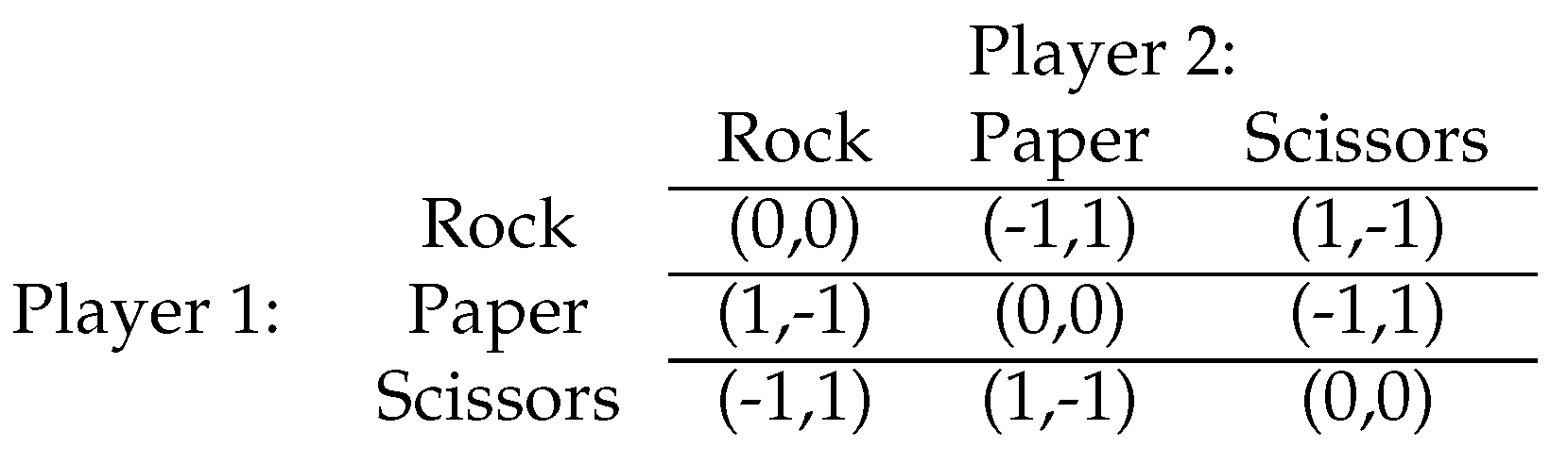
| 1 | Two players each play rock, paper, or scissors. Rock beats scissors; scissors beats paper; paper beats rock. If they both play the same, it is a tie. The payoff matrix is in Section 2. |
| 2 | If the opponent is not playing Nash, then Nash is no longer a best response. In symmetric zero-sum games such as RPS, deviating from Nash is costless if the opponent is playing Nash (since all strategies have an expected payoff of zero), but if a player thinks he knows what non-Nash strategy his opponent is using then there is a profitable deviation from Nash. |
| 3 | Work in evolutionary game theory on RPS has looked at how the population’s distribution of strategies evolves towards or around Nash equilibrium (e.g., [7,8]). Past work on fictitious play has showed that responding to the opponents’ historical frequency of strategies leads to convergence to Nash equilibrium [9,10,11]. Young [12] also studies how conventions evolve as players respond to information about how their opponents have behaved in the past, while Mookherjee and Sopher [13,14] examine the effect of information on opponents’ history on strategic choices. |
| 4 | When doing a test at the player level, we expect about 5% of players to be false positives, so we take these numbers as evidence on behavior only when they are statistically significant for substantially more than 5% of players. |
| 5 | Since the focal strategies can be skewed, our and strategies usually designate a unique throw, which would not be true if were constrained to be a uniform distribution. |
| 6 | As we discuss in Section 4, there are several reasons that may explain why we find lower estimates for and play than in previous work. Many players may not remember their own history, which is necessary for playing . Also, given that is what players would most likely play if they were not shown the information (i.e., when they play RPS outside the application), it may be more salient than in other contexts. |
| 7 | Because we think players differ in the extent to which they respond to information and consider expected payoffs, we do not impose the restriction from quantal response equilibrium theory [30] that the perceived expected payoffs are correct. Instead, we require that the expected payoffs are calculated based on the history of play. See Section 5 for more detail. |
| 8 | RPS is usually played for low stakes, but sometimes the result carries with it more serious ramifications. During the World Series of Poker, an annual $500 per person RPS tournament is held, with the winner taking home $25,000. RPS was also once used to determine which auction house would have the right to sell a $12 million Cezanne painting. Christie’s went to the 11-year-old twin daughters of an employee, who suggested “scissors” because “Everybody expects you to choose ‘rock’.” Sotheby’s said that they treated it as a game of chance and had no particular strategy for the game, but went with “paper” [31]. |
| 9 | Bart Johnston, one of the developers said, “We’ve added this intriguing statistical aspect to the game…You’re constantly trying to out-strategize your opponent” [32]. |
| 10 | Unfortunately we only have a player id for each player; there is no demographic information or information about their out-of-game connections to other players. |
| 11 | Because of the possibility for players to collude to give one player a good record if the other does not mind having a bad one, we exclude matches from the small fraction of player-pairs for which one player won an implausibly high share of the matches (100% of ≥10 games or 80% of ≥20 games). To accurately recreate the information that opponents were shown when those players played against others, we still include those “collusion” matches when forming the players’ histories. |
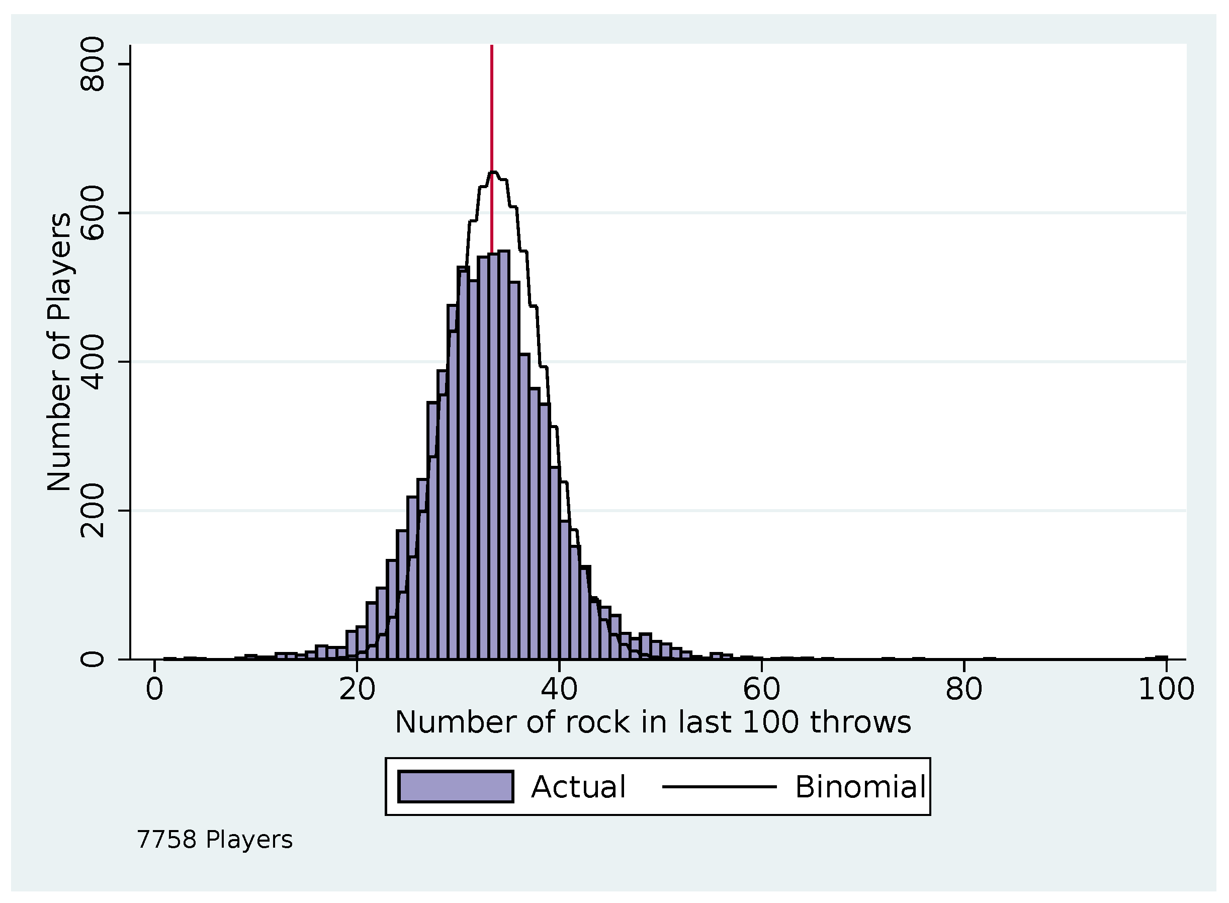
| 12 | Depending on the opponent’s history, the strategies we look at may not indicate a unique throw (e.g., if rock and paper have the same expected payoffs); for some analyses we only use players who have 100 clean matches where the strategies being considered indicate a unique throw, so we use between 5405 and 7758 players. |
| 13 | Players could use aspects of their history that are not observable to the opponent as a private randomization devices, but conditional on all information available to the opponent, they must be mixing . |
| 14 | We also find serial correlation both across throws within a match and across matches, which is inconsistent with Nash equilibrium. |
| 15 | Inexperienced players also have a lot of variance in the fraction of time they play rock, but for them it is hard to differentiate between deviations from and noise from randomization. |
| 16 | If all players were playing Nash, we would expect to reject the null for 5% of players; with 95% probability we would reject the null for less than 5.44% of players. |
| 17 | If players were truly, strictly maximizing their payoff against the opponent’s past distribution, this change would be even more stark, though it would not go exactly from 0 to 1 since the optimal response also depends on the percent of paper (or scissors) played, which the table does not condition on. |
| 18 | The Appendix A.2 has the same table adding own history. The coefficients on opponent’s history are basically unaffected. The coefficients on own history reflect the imperfect randomization—players who played rock in the past are more likely to play rock. |
| 19 | If we run the regression with just the distribution of all throws or just the lags, the signs are as expected, but that seems to be mostly picking up the effect via the opponent’s distribution of first throws. |
| 20 | The reduced-form results indicate that players react much more strongly to the distribution of first throws than to the other information provided. |
| 21 | Alternatively, a player may think that is strategic, but playing an unknown strategy so past play is the best predictor of future play. |
| 22 | Nash always has an expected payoff of zero. As show in Table 5, best responding can have an expected payoff of 14¢ for every dollar bet. |
| 23 | Sometimes opponents’ distributions are such that there are multiple throws that are tied for the highest expected payoff. For our baseline specification we ignore these throws. As a robustness check we define alternative -strategies where one throw is randomly chosen to be the throw when payoffs are tied or where both throws are considered consistent with when payoffs are tied. The results do not change substantially. |
| 24 | In the proof of Proposition 1 we show that in Nash equilibrium, histories do not affect continuation values, so in equilibrium it is a result, not an assumption, that players are myopic. However, out of Nash equilibrium, it is possible that what players throw now can affect their probability of winning later rounds. |
| 25 | One statistic that we thought might affect continuation values is the skew of a player’s historical distribution. As a player’s history departs further from random play, there is more opportunity for opponent response and player exploitation of opponent response. We ran multinomial logits for each experienced player on the effect of own history skewness on the probability of winning, losing, or drawing. The coefficients were significant for less than (the expected false positives of) 5% of players. This provides some support to our assumption that continuation values are not a primary concern. |
| 26 | As an aside, in the case of RPS the level strategy is identical to the level strategy for , so it is impossible to identify levels higher than 6. One might expect to be equivalent to , but , and strategies depend on the opponent’s history, with one being rock, one being paper, and one being scissors, while levels , and strategies depend on one’s own history. So, with many games all strategies with are separately identified. This also implies that the play we observe could in fact be play, but we view this as highly unlikely. |
| 27 | Since we do the analysis within player, the estimates would be very imprecise for players with fewer games. |
| 28 | We derive the Hessian of the likelihood function, plug in the estimates, and take the inverse. |
| 29 | Other work, such as [35], has found evidence of players mixing levels of sophistication across different games. |
| 30 | To fully calculate the equilibrium, we could repeat the analysis using the frequencies of and found below and continue until the frequencies converged, but since the estimated and are near the 79% and 20% we started with, we do not think this computationally intense exercise would substantially change the results. |
| 31 | Wright and Leyton-Brown [40]’s estimates are closer to ours, with 95% confidence interval for the average number of iterative steps of [0.51, 0.59]. |
| 32 | Similar predictions could be made about play; however, since we find that is used so little, we do not model play in this section. See Appendix A.2 |
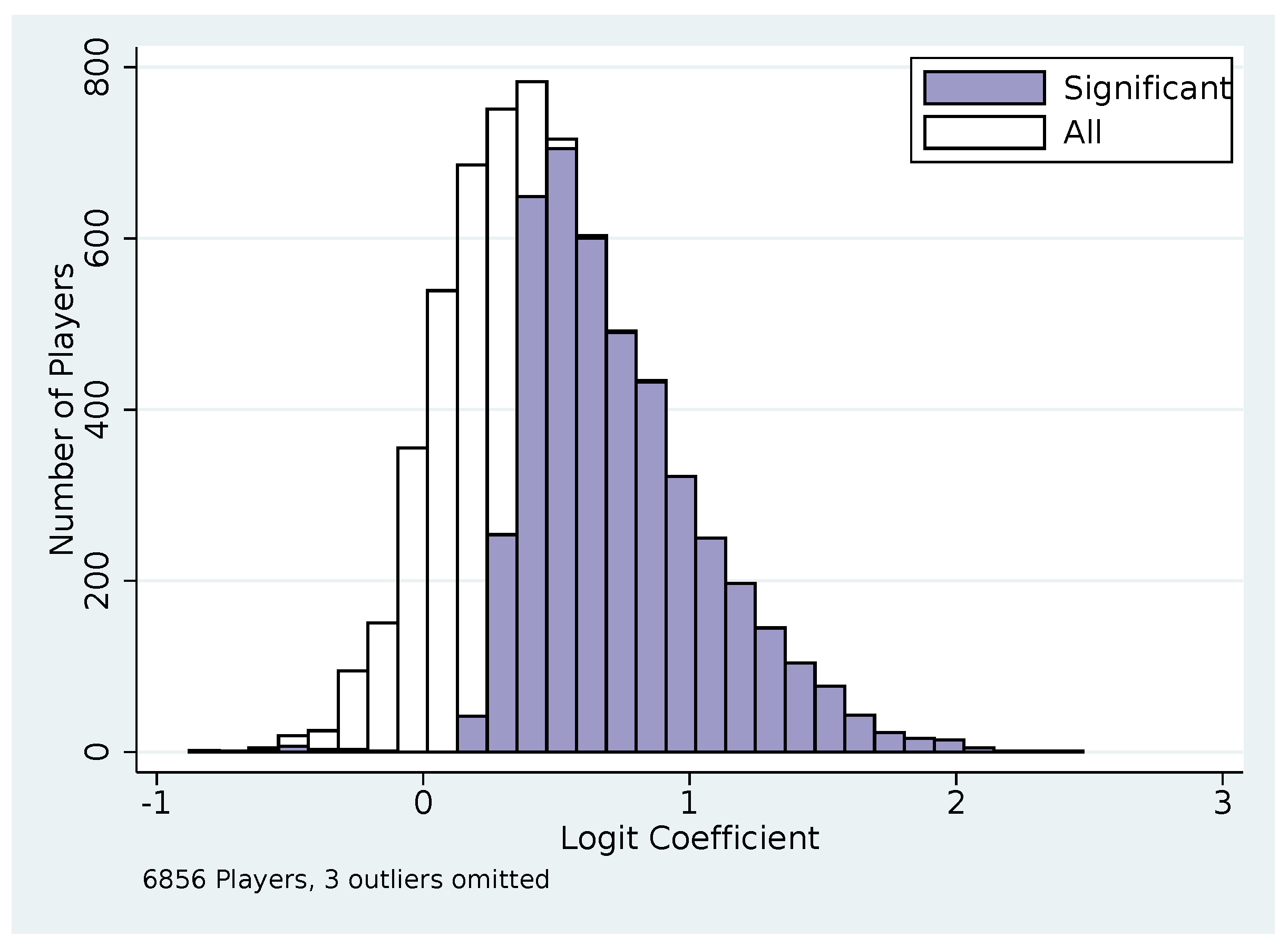
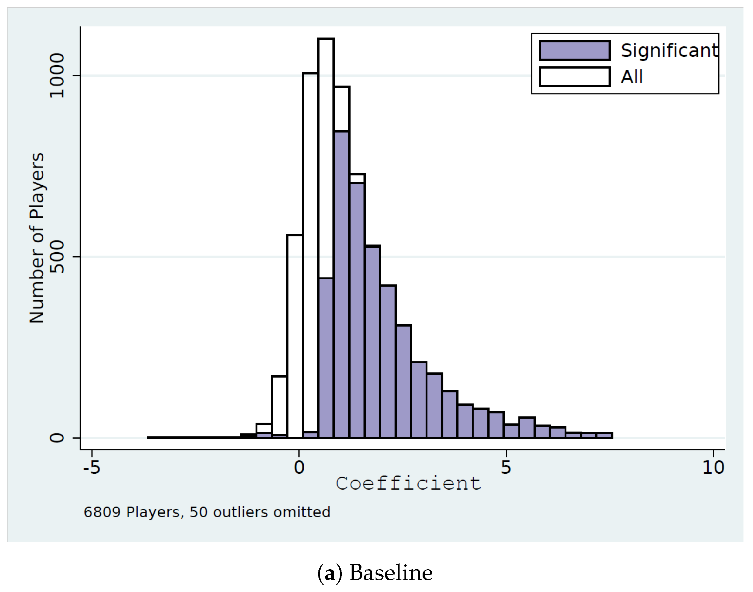
| 33 | We present OLS coefficients instead of logit, so they will be comparable when we add fixed-effects, which do not work with logit. When running logits at the player level, the median coefficients are in the range of the above coefficients, but the model is totally lacking power—the coefficients are significant for less than 5% of players. |
| 34 | If we allowed the expected payoff to vary or be estimated from the data, this would increase the flexibility of the model, making any improvement in fit suspect. However, since the expected payoff is completely determined by the opponent’s historical distribution the model has only 3 free parameters—estimated separately for each player—the and two s. (The third is normalized to zero.) |
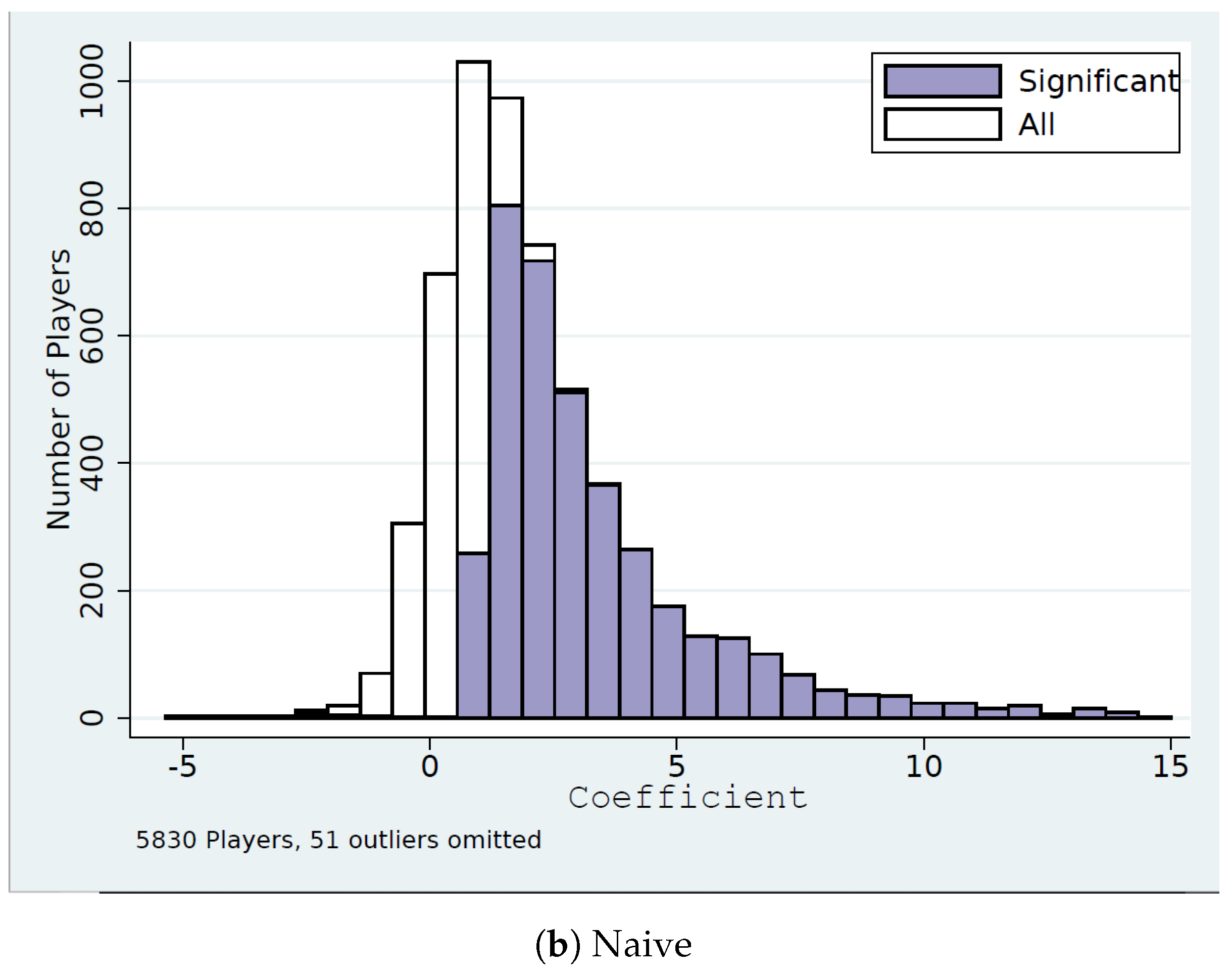
| 35 | A second level of reasoning would expect opponents to play according to the distribution induced by one’s own history and would play with probabilities proportional to the expected payoff against that distribution. However, given the low levels of play we find and the econometric difficulties of including own history in the logit, we only analyze the first iteration of reasoning. |
| 36 | This suggests that players do respond to expected payoffs calculated from historical opponent play; whereas in the reduced-form results (Table 4) we showed that players did not respond to the expected payoff calculated from predicted opponent play—predicted based on the coefficients from Table 3 and players’ histories. |
| 37 | We multiply by 100 to convert to percentages and by 2/9 to evaluate the margin at the mean: . |
| 38 | Models with additional parameters have more flexibility to fit data better even when the underlying model is no better. We find little evidence of and using a model avoids choosing how much to penalize the level-k model for the additional parameter. |
| 39 | This would be an interesting dimension for future work to explore. |
| 40 | In the actual game players could challenge a specific player to a game or be matched by the software to someone else who was looking for an opponent. |
| 41 | Because what matters for the result is the symmetry across strategies at all stages, having an intra-match discount factor does not change the result, but substantially complicates the proof. |


| Variable | Full Sample | Restricted Sample | ||
|---|---|---|---|---|
| Mean | (SD) | Mean | (SD) | |
| Throw Rock (%) | 33.99 | (47.37) | 32.60 | (46.87) |
| Throw Paper (%) | 34.82 | (47.64) | 34.56 | (47.56) |
| Throw Scissors (%) | 31.20 | (46.33) | 32.84 | (46.96) |
| Player’s Historical %Rock | 34.27 | (19.13) | 32.89 | (8.89) |
| Player’s Historical %Paper | 35.14 | (18.80) | 34.88 | (8.97) |
| Player’s Historical %Scissors | 30.59 | (17.64) | 32.23 | (8.57) |
| Opp’s Historical %Rock | 34.27 | (19.13) | 33.59 | (13.71) |
| Opp’s Historical %Paper | 35.14 | (18.80) | 34.76 | (13.46) |
| Opp’s Historical %Scissors | 30.59 | (17.64) | 31.65 | (12.84) |
| Opp’s Historical Skew | 10.42 | (18.08) | 5.39 | (12.43) |
| Opp’s Historical %Rock (all throws) | 35.45 | (12.01) | 34.81 | (8.59) |
| Opp’s Historical %Paper (all throws) | 34.01 | (11.74) | 34.10 | (8.35) |
| Opp’s Historical %Scissors (all throws) | 30.54 | (11.07) | 31.09 | (7.98) |
| Opp’s Historical Length (matches) | 55.92 | (122.05) | 99.13 | (162.16) |
| Total observations | 5,012,128 | 1,472,319 | ||
| Opp’s Historical % | Throws (%) | N | ||
|---|---|---|---|---|
| Paper | Rock | Scissors | ||
| 0%–25% | 27.07 | 35.84 | 37.09 | 1,006,726 |
| 25%–30% | 27.11 | 35.23 | 37.66 | 728,408 |
| 30%–% | 29.87 | 34.72 | 35.41 | 565,623 |
| %–37% | 34.21 | 34.44 | 31.35 | 794,886 |
| 37%–42% | 40.45 | 32.58 | 26.97 | 529,710 |
| 42%–100% | 46.58 | 30.35 | 23.06 | 1,056,162 |
| Covariate | Dependent Var: Dummy for Throwing Rock | ||
|---|---|---|---|
| (1) | (2) | (3) | |
| Opp’s Fraction Paper (first) | −0.0382 *** | −0.0729 *** | −0.0955 *** |
| (0.0021) | (0.0056) | (0.0087) | |
| Opp’s Fraction Scissors (first) | 0.2376 *** | 0.1556 *** | 0.1381 *** |
| (0.0022) | (0.0060) | (0.0094) | |
| Opp’s Fraction Paper (all) | 0.0011 | 0.0258 ** | 0.0033 |
| (0.0032) | (0.0088) | (0.0138) | |
| Opp’s Fraction Scissors (all) | 0.0416 *** | 0.0231 * | −0.0208 |
| (0.0033) | (0.0093) | (0.0146) | |
| Opp’s Paper Lag | 0.0052 *** | −0.0019 | −0.0043 * |
| (0.0007) | (0.0015) | (0.0019) | |
| Opp’s Scissors Lag | 0.0139 *** | 0.0055 *** | −0.0017 |
| (0.0008) | (0.0016) | (0.0020) | |
| Own Paper Lag | −0.0171 *** | 0.0239 *** | 0.0051 ** |
| (0.0007) | (0.0015) | (0.0019) | |
| Own Scissors Lag | −0.0145 *** | 0.0208 *** | −0.0047 * |
| (0.0007) | (0.0015) | (0.0019) | |
| Constant | 0.3548 *** | −0.0264 *** | −0.0009 |
| (0.0006) | (0.0014) | (0.0018) | |
| 0.0172 | |||
| N | 4,433,260 | ||
| Opponent’s Expected Payoff of Rock | Opponent’s Throw (%) | N | ||
|---|---|---|---|---|
| Paper | Rock | Scissors | ||
| 30.83 | 40.56 | 28.61 | 2754 | |
| 32.89 | 38.56 | 28.55 | 65,874 | |
| 33.83 | 34 | 32.17 | 1,266,538 | |
| 35.52 | 32.45 | 32.03 | 871,003 | |
| 34.4 | 34.47 | 31.13 | 12,234 | |
| Wins (%) | Draws (%) | Losses (%) | Wins (%) − Losses (%) | N | |
|---|---|---|---|---|---|
| Full Sample | 33.8 | 32.4 | 33.8 | 0 | 5,012,128 |
| Experienced Sample | 34.66 | 32.17 | 33.17 | 1.49 | 1,472,319 |
| Best Response to Predicted Play | 41.66 | 30.97 | 27.37 | 14.29 | 2,218,403 |
| Variable | Definition |
|---|---|
| fraction of the time a player plays and chooses rock | |
| fraction of the time a player plays and chooses paper | |
| fraction of the time a player plays and chooses scissors | |
| fraction of the time a player plays | |
| (not an independent parameter) |
| Variable | Mean | SD | Median | Min | Max |
|---|---|---|---|---|---|
| 0.738 | 0.16 | 0.75 | 0.19 | 1.00 | |
| 0.185 | 0.14 | 0.16 | 0.00 | 0.77 | |
| 0.077 | 0.08 | 0.06 | 0.00 | 0.41 | |
| N = 6639 | |||||
| Variable | 95% CI Does Not Include 0 | 95% CI Does Not Include 1 | 95% CI Does Not Include 0 or 1 |
|---|---|---|---|
| 93.11% | 58.30% | 57.51% | |
| 62.87% | 99.97% | 62.87% | |
| 11.54% | 95.57% | 11.54% | |
| N = 6389 | |||
| Variable | Mean | SD | Median | Min | Max |
|---|---|---|---|---|---|
| 0.750 | 0.16 | 0.77 | 0.17 | 1.00 | |
| 0.161 | 0.14 | 0.14 | 0.00 | 0.77 | |
| 0.089 | 0.07 | 0.08 | 0.00 | 0.49 | |
| N = 6856 | |||||
| Variable | Mean | SD | Median | Min | Max |
|---|---|---|---|---|---|
| 0.722 | 0.18 | 0.75 | 0.07 | 1.00 | |
| 0.211 | 0.17 | 0.18 | 0.00 | 0.93 | |
| 0.067 | 0.08 | 0.04 | 0.00 | 0.46 | |
| N = 5692 | |||||
| Model | |||
|---|---|---|---|
| Level-k | Cognitive Hierarchy | Naive | |
| All Players | 798 | 1833 | 2629 |
| 14.8% | 33.9% | 48.6% | |
| Players Prob | 13 | 188 | 1148 |
| 1.0% | 13.9% | 85.1% | |
| (1) | (2) | (3) | |
|---|---|---|---|
| K1 Payoff | 0.068 *** | 0.105 *** | 0.071 *** |
| (0.0012) | (0.0013) | (0.0016) | |
| High Opponent Experience | −0.076 *** | ||
| (0.0017) | |||
| Medium Opponent Experience | −0.055 *** | ||
| (0.0015) | |||
| K1 Payoff X High Opponent Experience | 0.528 *** | ||
| (0.010) | |||
| K1 Payoff X Medium Opponent Experience | 0.318 *** | ||
| (0.0050) | |||
| Experienced | 0.015 *** | ||
| (0.0015) | |||
| Exp X Payoff from Playing K1 | 0.068 *** | 0.041 *** | −0.021 *** |
| (0.0039) | (0.0038) | (0.0046) | |
| Exp X High Opponent Experience | −0.019 *** | ||
| (0.0034) | |||
| Exp X Medium Opponent Experience | −0.023 *** | ||
| (0.0035) | |||
| Exp X K1 Payoff X High Opponent Experience | 0.091 *** | ||
| (0.021) | |||
| Exp X K1 Payoff X Medium Opponent Experience | 0.095 *** | ||
| (0.013) | |||
| Own Games>100 | −0.002 | ||
| (0.0022) | |||
| Own Games>100 X Payoff from Playing K1 | 0.082 *** | 0.072 *** | 0.021 *** |
| (0.0068) | (0.0050) | (0.0049) | |
| Own Games>100 X High Opponent Experience | 0.012 *** | ||
| (0.0026) | |||
| Own Games>100 X Medium Opponent Experience | 0.022 *** | ||
| (0.0035) | |||
| Own Games>100 X K1 Payoff X High Opponent Experience | −0.025 | ||
| (0.023) | |||
| Own Games>100 X K1 Payoff X Medium Opponent Experience | 0.014 | ||
| (0.016) | |||
| Player Fixed Effects | No | Yes | Yes |
| Observations | 4,130,024 | 4,130,024 | 4,130,024 |
| Adjusted | 0.003 | 0.004 | 0.008 |
| All Players | Players with Significant Difference | |||
|---|---|---|---|---|
| Regular | Naive | Regular | Naive | |
| Est. MLE fraction play | 3.451 *** | 2.707 *** | 3.417 *** | 2.619 *** |
| (0.0569) | (0.0524) | (0.0661) | (0.0641) | |
| Est. QR coefficient on return to | −0.284 *** | −0.106 *** | −0.248 *** | −0.0870 *** |
| (0.0054) | (0.0029) | (0.0051) | (0.0027) | |
| Total Number of Matches (100s) | 0.0200 *** | 0.0168 *** | 0.0238 *** | 0.0131 * |
| (0.0036) | (0.0042) | (0.0041) | (0.0051) | |
| Constant | 0.173 *** | 0.208 *** | 0.0549 ** | 0.135 *** |
| (0.0106) | (0.0120) | (0.0192) | (0.0221) | |
| 0.358 | 0.321 | 0.565 | 0.438 | |
| N | 6673 | 5731 | 2373 | 2216 |
© 2019 by the authors. Licensee MDPI, Basel, Switzerland. This article is an open access article distributed under the terms and conditions of the Creative Commons Attribution (CC BY) license (http://creativecommons.org/licenses/by/4.0/).
Share and Cite
Batzilis, D.; Jaffe, S.; Levitt, S.; List, J.A.; Picel, J. Behavior in Strategic Settings: Evidence from a Million Rock-Paper-Scissors Games. Games 2019, 10, 18. https://doi.org/10.3390/g10020018
Batzilis D, Jaffe S, Levitt S, List JA, Picel J. Behavior in Strategic Settings: Evidence from a Million Rock-Paper-Scissors Games. Games. 2019; 10(2):18. https://doi.org/10.3390/g10020018
Chicago/Turabian StyleBatzilis, Dimitris, Sonia Jaffe, Steven Levitt, John A. List, and Jeffrey Picel. 2019. "Behavior in Strategic Settings: Evidence from a Million Rock-Paper-Scissors Games" Games 10, no. 2: 18. https://doi.org/10.3390/g10020018
APA StyleBatzilis, D., Jaffe, S., Levitt, S., List, J. A., & Picel, J. (2019). Behavior in Strategic Settings: Evidence from a Million Rock-Paper-Scissors Games. Games, 10(2), 18. https://doi.org/10.3390/g10020018