Agency Equilibrium ^†

Abstract

Agency may be exercised by different entities (e.g., individuals, firms, households). A given individual can form part of multiple agents (e.g., he may belong to a firm and a household). The set of agents that act in a given situation might not be common knowledge. We adapt the standard model of incomplete information to model such situations.

1. Introduction

The doctrine of methodological individualism (see [1]) is that social phenomena should be explained with reference to the actions of individual agents and the intentional states (e.g., belief, desire, hope, intention) that motivate these actions. Early proponents of methodological individualism [2,3] regarded individual people (henceforth, individuals) as the only entities that could hold intentional states and consequently held that social theory should be founded upon individual agency. However, in practice, social scientists often model collective entities (households, firms) or intra-human entities (multiple selves) as agents. 1

This is consistent with methodological individualism if such agents can hold intentional states or, in the sense of positive methodology [6,7], can act as if they hold intentional states. 2^,3

The above raises the prospect of an individual forming part of multiple agents with conflicting interests. Consider, for example, a firm with two partners, Alice and Bob, who sometimes make decisions together with the goal of maximizing the firm’s profits, but who also sometimes make decisions as singletons with the goal of furthering their own interests. Such conflicts of interest define the Prisoner’s Dilemma (see [13]) and the Tragedy of the Commons [14,15]. Furthermore, an individual might not know the agents to which other individuals belong. Colm may know that Alice and Bob are partners, but in some specific situation be unsure over whether they will make a decision together or make separate decisions. Colm is unsure about whether he faces one other agent or two other agents.

Here, we extend the concept of Bayesian Nash Equilibrium [16,17,18] to deal with incomplete information about the identity of agents in a game. In agency equilibrium, a random state of the world determines not only payoffs, but also a set of agents whose incentive constraints must be satisfied. Each agent comprises either a single individual (individual agency) or a set of individuals (collective agency). If the set of agents equals the set of singletons at every state, then the solution reduces to Bayesian Nash Equilibrium. If the set of agents is the same at every state and agents maximize the utilitarian welfare of their constituent individuals, the solution reduces to (Bayesian) coalitional equilibrium in the sense of [19]. 4 Every finite game of incomplete information is shown to have at least one agency equilibrium in pure or mixed strategies (Theorem 1).

Agency equilibrium is used to explore the implications of uncertainty over agency across several examples. In Cournot oligopoly, the possibility that other firms might have formed a secret cartel leads to singleton firms increasing their production, so that even in the absence of cartels, total production is higher than it would be in the model with complete information.

In coordination games [22,23], the possibility that other individuals are solving the coordination problem directly through explicit agreement can eliminate inefficient equilibria, even at states at which there is no collective agency. It is known that Nash equilibria can be non-robust to even vanishingly small amounts of uncertainty over payoffs [24]. Here, it is shown that this non-robustness extends to small amounts of uncertainty over agency. That is, even the smallest possibility of collective agency may suffice to ensure that the agency equilibrium outcome is far from the Nash equilibrium outcome of the game under complete information.

It may sometimes be preferable to dispense with the necessity and accompanying flexibility of defining payoffs for collective agents (see discussion in Section 5). To this end, Pareto agency equilibrium is defined to rely upon Pareto dominance arguments and explicitly eschew interpersonal comparability of payoffs. Agency equilibrium and Pareto agency equilibrium are closely related. Any agency equilibrium under utilitarian payoffs is also a Pareto agency equilibrium (Proposition 1). For finite games of incomplete information, the existence of agency equilibrium then implies the existence of Pareto agency equilibrium (Theorem 2). Moving in the opposite direction, any Pareto agency equilibrium is an agency equilibrium under some utilitarian payoffs (Proposition 2). These concepts are illustrated through the examples of the prisoner’s dilemma and an extended version of the battle of the sexes.

The most similar model in the literature is that of [25], the primary interest of which is situations where the membership of a collective (a ‘team’) is unreliable. For example, Alice may reason and act according to the perspective of a firm she co-owns with Bob, even though Bob is unreliable and sometimes reasons from an individual perspective. In contrast, here we focus on the case in which individuals within a collective agent are reliable. That is, both Alice and Bob know whether they are making decisions together or as individuals and act accordingly. The subtlety arises from the uncertainty of others over the agency of Alice and Bob. Ref. [25] can thus be seen as an analysis of individuals reasoning in isolation but taking the perspective of a collective 5, whereas the current model considers the strategic implications of the uncertain possibility of explicit face-to-face collective deliberation.

The literature on cooperative games under incomplete information (see, e.g., Refs. [31,32,33,34,35]) also considers the two concepts of collective agency and incomplete information, but combines them in a very different way. Specifically, it considers coalitions that exhibit agency and then analyzes the incentive compatibility of information sharing within such coalitions. It is assumed that Alice and Bob form an agent, but the payoffs attainable by this agent depend on the individual incentives of Alice and Bob to share information about the state of the world with one another. In contrast, the current paper analyzes incomplete information over which coalitions exhibit agency, assuming information sharing within those coalitions. Alice and Bob may or may not form an agent, and this information may be unknown to third parties, but when they do form an agent, the information that they share about the state of the world is exogenously given. This understood, the current paper can be considered as a fresh approach to incomplete information in cooperative games, focusing on strategic externalities that have been largely neglected in the literature (see discussion in [36]).

This paper is organized as follows. Section 2 describes games with incomplete information over agency, defines, discusses and shows the existence of agency equilibrium. Section 3 applies the concept to several examples, including demonstrating the potential non-robustness of Nash equilibrium to small amounts of incomplete information over agency. Section 4 defines, discusses and shows the existence of Pareto agency equilibrium, as well as giving conditions under which an agency equilibrium is a Pareto agency equilibrium and vice versa. Section 5 briefly discusses the merits of agency equilibrium and Pareto agency equilibrium with respect to one another.

2. Model

An incomplete information game $\mathcal{U}$ consists of (1) the set of individuals, $\mathcal{I}=\{1,\dots ,I\}$; (2) the individuals’ action sets, $A_1,\dots ,A_I$, with $A=A_1\times \dots \times A_I$ a topological space; (3) a countable state space, $\Omega$; (4) a probability measure on the state space, P; (5), for each individual i, a partition of the state space, ${\mathcal{Q}}_i$; and (6), for each individual i, a bounded, measurable, state-dependent payoff function, $u_i:A\times \Omega \to \mathbb{R}$. Thus, $\mathcal{U}=\{\mathcal{I},{\left\{A_i\right\}}_{i\in \mathcal{I}},\Omega ,P,{\left\{{\mathcal{Q}}_i\right\}}_{i\in \mathcal{I}},{\left\{u_i\right\}}_{i\in \mathcal{I}}\}$. We write $P\left(\omega \right)$ for the probability of the singleton event $\left\{\omega \right\}$ and $Q_i\left(\omega \right)$ for the (unique) element of ${\mathcal{Q}}_i$ containing $\omega$. We restrict attention to games where every information set of every individual is possible, that is $P\left[Q_i\left(\omega \right)\right]>0$ for all $i\in \mathcal{I}$ and $\omega \in \Omega$. Hence, the conditional probability of state $\omega$ given information set $Q_i\left(\omega \right)$, written $P\left[\omega \right|Q_i\left(\omega \right)]$, is well-defined by the rule $P\left[\omega \right|Q_i\left(\omega \right)]=P\left(\omega \right)/P\left[Q_i\left(\omega \right)\right]$. Where relevant, we will assume that A is endowed with the Borel sigma-algebra and $\Omega$ is endowed with its power set as a sigma-algebra.

This description is a standard description of a game of incomplete information (see, e.g., [24]). However, for our purposes, we require two further objects. (7) An agency correspondence $\Pi :\Omega \rightrightarrows \mathcal{P}\left(\mathcal{I}\right)$ such that $\Pi \left(\omega \right)$ is a partition of $\mathcal{I}$ into agents. As a set of agents $\Pi \left(\omega \right)$ is a partition of $\mathcal{I}$, we have that, at any given state $\omega$, individual i is a member of exactly one agent. Further restrict $\Pi$ so that if $i\in J\in \Pi \left(\omega \right)$ and ${\omega }^{\prime }\in Q_i\left(\omega \right)$, then $J\in \Pi \left({\omega }^{\prime }\right)$. That is, the agent to which individual i belongs is constant across states in information set $Q_i\left(\omega \right)$, $\omega \in \Omega$. (8) For each agent $J\subseteq \mathcal{I}$, a bounded, measurable, state-dependent payoff function, $v_J:A\times \Omega \to \mathbb{R}$, such that $v_{\left\{i\right\}}=u_i$ for all $i\in \mathcal{I}$. This specifies the payoffs according to which agents make decisions. It is restricted so that when an agent is a single individual, the agent’s payoff function is identical to that of the individual concerned. In some instances, it will be natural to define $v_J$ in terms of $u_i$, for example, when agents have utilitarian payoffs $v_J(a,\omega )={\sum }_{i\in J}{\lambda }_i\left(\omega \right)u_i(a,\omega )$, where ${\lambda }_i\left(\omega \right)$ are strictly positive, possibly state-dependent welfare weights.

For $J\subseteq \mathcal{I}$, write $A_J={\prod }_{i\in J}{A}_i$. Let ${\mathcal{Q}}_J$ be the coarsest common refinement of ${\mathcal{Q}}_i$, $i\in J$. That is, ${\mathcal{Q}}_J$ is a pooling of the information that individuals in J have about the state of the world. A strategy for agent $J\subseteq \mathcal{I}$ is a ${\mathcal{Q}}_J$-measurable function ${\sigma }_J:\{\Omega :J\in \Pi \left(\omega \right)\}\to \Delta A_J$, where $\Delta A_J$ is the set of probability measures on the Borel sets of $A_J$. We write ${\Sigma }_J$ for the set of such strategies. A strategy profile is a function $\sigma :\Omega \to \Delta A$ such that $\sigma \left(\omega \right)={\left({\sigma }_J\left(\omega \right)\right)}_{J\in \Pi \left(\omega \right)}$, where ${\sigma }_J$ is a strategy for agent J. Let $\Sigma$ denote the set of all strategy profiles. Given $\omega$ such that $J\in \Pi \left(\omega \right)$, we write ${\sigma }_{-J}\left(\omega \right)$ for ${\left({\sigma }_K\left(\omega \right)\right)}_{K\in \Pi \left(\omega \right)\setminus \left\{J\right\}}$. When no confusion arises, we extend the domain of each $v_J$ to mixed strategies and thus write $v_J(\sigma \left(\omega \right),\omega )$ for ${\int }_{a\in A}{v}_J(a,\omega )\mathrm{d}\sigma \left(a\right|\omega )$. Similarly, we extend the domain of each $u_i$ to mixed strategies and write $u_i(\sigma \left(\omega \right),\omega )$ for ${\int }_{a\in A}{u}_i(a,\omega )\mathrm{d}\sigma \left(a\right|\omega )$.

Definition 1.

Given game $\mathcal{U}$, agents’ payoffs v, strategy profile $\sigma \in \Sigma$, state of the world $\omega \in \Omega$, then $a_J\in A_J$ is a profitable deviation for $J\in \Pi \left(\omega \right)$ if

$$\begin{array}{c}\sum _{{\omega }^{\prime }\in Q_J\left(\omega \right)}{v}_J(\{a_J,{\sigma }_{-J}\left({\omega }^{\prime }\right)\},{\omega }^{\prime })P\left[{\omega }^{\prime }\right|Q_J\left(\omega \right)]\hfill \\ >\sum _{{\omega }^{\prime }\in Q_J\left(\omega \right)}{v}_J(\sigma \left({\omega }^{\prime }\right),{\omega }^{\prime })P\left[{\omega }^{\prime }\right|Q_J\left(\omega \right)].\hfill \end{array}$$

Definition 2.

A strategy profile σ is an Agency Equilibrium of $(\mathcal{U},\Pi ,v)$ if, for all $\omega \in \Omega$, no profitable deviation exists for any $J\in \Pi \left(\omega \right)$.

Remark 1.

If σ is an agency equilibrium of $(\mathcal{U},{\Pi }^{NE},v)$, where ${\Pi }^{NE}\left(\omega \right)=\{\left\{1\right\},\left\{2\right\},\dots ,\left\{I\right\}\}$ for all $\omega \in \Omega$, then ${\left({\sigma }_{\left\{i\right\}}\right)}_{i\in \mathcal{I}}$ is a Bayesian Nash Equilibrium [17] of $\mathcal{U}$.

Remark 2.

The following two assumptions of the model are parallel. (i) An individual can potentially belong to many agents whose incentives may differ, but is only part of one agent at any given state. (ii) An individual can potentially have many preferences which may contradict one another, but has only one set of preferences at any given state. The first of these assumptions is the focus of this paper, so we will isolate its effect in our examples, all of which feature complete information over payoffs but incomplete information over agency.

Remark 3.

In agency equilibrium, an agent $J\subseteq \mathcal{I}$ is instrumentally rational [37] in that the strategy of J is chosen to achieve the “goals, desires, and ends” [38] of J, as represented by $v_J$. As [38] notes, “About the goals themselves, an instrumental conception has little to say.” In our examples, we let $v_J$ depend in a positive way on $u_i$, $i\in J$, but neither this, nor any other dependence on the individual payoffs is required by the model.

Remark 4.

The individuals within agent J can be regarded as the instruments of J with respect to the instrumentally rational intent of J to maximize $v_J$. This highlights the independence of agency and payoffs. For example, if $v_J={\sum }_{i\in J}{u}_i$, then the payoffs of J are entirely determined by the payoffs of its constituent individuals, yet the actions of the constituent individuals are entirely determined by J’s instrumentally rational pursuit of these payoffs.

Remark 5.

Given a state of the world, our model only allows an individual to be instrumentalized by a single agent. Hypothetically, if an individual were to be simultaneously (i.e., at a given state) instrumentalized by more than one agent, then there would have to be no conflict of interest between these agents regarding the desired action of the individual concerned. From this perspective, it is without loss of generality to restrict individuals to be part of only a single agent at any given state. When this is not the case, for example in the Strong Equilibrium concept of [39] in which every subset of $\mathcal{I}$ simultaneously exercises agency, equilibria may fail to exist due to conflicting incentives between agents. The same applies to Strong Equilibrium with incomplete information over payoffs [40] and to ideas of Coalition Proofness [41,42].

Remark 6.

The definition of ${\mathcal{Q}}_J$ assumes that agent J can use all of the information that is available to its constituent individuals. This assumption is justifiable (see Remark 7), but is not essential. An alternative assumption would be to only allow J to use information known already to every one of its constituent individuals, that is to define ${\mathcal{Q}}_J$ as the finest common coarsening of ${\mathcal{Q}}_i$, $i\in J$. Intermediate definitions of ${\mathcal{Q}}_J$ are likewise acceptable. The crucial point is that ${\mathcal{Q}}_J$ is exogenously determined. Here, we do not study the implications of incomplete information over payoffs on the incentive compatibility of information revelation by individuals within an agent see, e.g., [31,32,33,34,35], but rather the equilibrium implications of incomplete information about the identities of other agents.

Remark 7.

If $\Pi \left(\omega \right)$ is constant across all $\omega \in \Omega$ and $v_J={\sum }_{i\in J}{u}_i$ for all $J\subseteq \mathcal{I}$, then an agency equilibrium is a (Bayesian) Coalitional Equilibrium [19]. The cited paper shows that, if utility is transferable, then there exists a mechanism of transfers between individuals within an agent under which full information sharing is incentive compatible at an individual level.

Remark 8.

If mixed strategies are disallowed so that ${\sigma }_J\left(\omega \right)$ always puts all probability weight on a single action profile, then the model is a special case of the unreliable team interaction model of [25] under the restriction that if individual i reasons and acts from the perspective of collective J, then all individuals $j\in J$ reason and act from the perspective of J, and this is common knowledge amongst the individuals in J.

Remark 9.

An alternative approach to modeling multiple agency is to explicitly model adaptive dynamics in which a given individual may be part of different agents at different times [43,44,45,46,47,48,49,50]. Such models give a complete description of behavior both in and out of equilibrium.

An agency equilibrium will always exist for finite games, regardless of commonality or opposition in the optimal choices of agents. That is, an agency equilibrium will exist, regardless of whether Alice, Bob and Colm take the same or different actions contingent on acting singly, in pairs, or as a trio.

Theorem 1.

If $\mathcal{U}$ is such that Ω, $A_i$, $i\in \mathcal{I}$ are finite, then the set of agency equilibria of $(\mathcal{U},\Pi ,v)$ is nonempty.

The proof derives a finite game of complete information over both payoffs and agency from $(\mathcal{U},\Pi ,v)$. The player set is the finite set of agent-information set pairs, $(J,Q_J)$, $J\subseteq \mathcal{I}$, $Q_J\in {\mathcal{Q}}_J$, such that at any state $\omega \in Q_J$, J is an active agent, $J\in \Pi \left(\omega \right)$. Player $(J,Q_J)$ has finite action sets $A_J$ and payoffs corresponding to the expected payoff of J in $(\mathcal{U},\Pi ,v)$ at any state $\omega \in Q_J$. A Nash equilibrium of this derived game must exist [51]. Finally, it is shown that such a Nash equilibrium must correspond to an agency equilibrium of $(\mathcal{U},\Pi ,v)$. The formal proof introduces substantial new notation, which is not used elsewhere in the paper, so, for ease of reading, is relegated to Appendix A.

3. Applications

3.1. Cournot Oligopoly

Consider quantity competition between three firms 6, $\mathcal{I}=\{1,2,3\}$. Each firm $i\in \mathcal{I}$ chooses a production quantity $A_i={\mathbb{R}}_{\ge 0}$. Individual firms’ payoffs depend only on the quantities chosen by the firms and not on the state of the world, $u_i(a,\omega )=a_i(R-{\sum }_j{a}_j)$, $R>0$. Agents’ payoffs are utilitarian, $v_J(a,\omega )={\sum }_{i\in J}{u}_i(a,\omega )$ for all $J\subseteq I$.

The state space is $\Omega =\{{\omega }_0,{\omega }_1,{\omega }_2,{\omega }_3\}$. At state ${\omega }_0$, no firms form a cartel, $\Pi \left({\omega }_0\right)=\{\left\{1\right\},\left\{2\right\},\left\{3\right\}\}$. At state ${\omega }_i$, $i=1,2,3$, firm i produces on his own and the other two firms form a cartel, $\Pi \left({\omega }_i\right)=\{\left\{i\right\},\{j,k\}\}$, $j,k\ne i$. Let each of the three pairs that can form a cartel do so with probability $p<\raisebox{1ex}{$1$}\!\left/ \!\raisebox{-1ex}{$3$}\right.$, so $P\left({\omega }_0\right)=1-3p$, $P\left({\omega }_i\right)=p$ for $i=1,2,3$.

The information structure is such that if firm i is not part of a cartel, then firm i does not know whether or not firms j and k form a cartel. Firms that are part of a cartel know this and hence know the exact state of the world. Therefore, ${\mathcal{Q}}_i=\{\{{\omega }_0,{\omega }_i\},\left\{{\omega }_j\right\},\left\{{\omega }_k\right\}\}$.

Consider an agency equilibrium which is symmetric in that both members of any cartel produce the same quantity. For $i=1,2,3$, $i\notin J=\{j,k\}$, we obtain equilibrium strategies ${\sigma }_i\left(a_0\right|{\omega }_0)=1$, ${\sigma }_i\left(a_i\right|{\omega }_i)=1$, ${\sigma }_J\left((a_j,a_k)\right|{\omega }_i)=1$, where

$$a_0=a_i=\frac{2-5p}{8-21p},a_j=a_k=\frac{3-8p}{16-42p}.$$

At state ${\omega }_i$, firms j and k form a cartel and reduce their production. At states ${\omega }_0$, ${\omega }_i$, firm i does not know whether j and k are in fact part of a cartel, but knowing that this is a possibility, increases production as a consequence. Note that at state ${\omega }_0$, at which there is no cartel, every firm produces more than the Nash equilibrium quantity of $\raisebox{1ex}{$1$}\!\left/ \!\raisebox{-1ex}{$4$}\right.$. As $p\to 0$, $P\left({\omega }_0\right)\to 1$, cartels become a rare occurrence and $a_0\to \raisebox{1ex}{$1$}\!\left/ \!\raisebox{-1ex}{$4$}\right.$. Conversely, as $p\to \raisebox{1ex}{$1$}\!\left/ \!\raisebox{-1ex}{$3$}\right.$, we have that $P\left({\omega }_0\right)\to 0$ and a cartel is almost a certainty. Production by both solo firms and cartels then approaches the Nash equilibrium quantity of the two-firm model, $a_i\to \raisebox{1ex}{$1$}\!\left/ \!\raisebox{-1ex}{$3$}\right.$, $a_j+a_k\to \raisebox{1ex}{$1$}\!\left/ \!\raisebox{-1ex}{$3$}\right.$.

3.2. Coordination Game: Hi-Lo

Let there be three individuals, $\mathcal{I}=\{1,2,3\}$ with action sets $A_i=\{H,L\}$. For each state of the world $\omega$, let $u_i(a,\omega )=2$ (respectively, 1) if $a_i=H$ (respectively, L) and $a_j=a_i$ for some $j\ne i$. Otherwise, $u_i(a,\omega )=0$. That is, an individual obtains payoff from successfully coordinating on H or L with at least one other individual, with coordination on H giving a payoff of 2 and coordination on L giving a payoff of 1. Agents’ payoffs are utilitarian with arbitrary state-dependent weightings, $v_J(a,\omega )={\sum }_{i\in J}{\lambda }_i\left(\omega \right)u_i(a,\omega )$ for all $J\subseteq I$, where ${\lambda }_i\left(\omega \right)>0$ for every $i\in J$, $\omega \in \Omega$.

As in the previous example, the state space is $\Omega =\{{\omega }_0,{\omega }_1,{\omega }_2,{\omega }_3\}$, $\Pi \left({\omega }_0\right)=\{\left\{1\right\},\left\{2\right\},\left\{3\right\}\}$, and for ${\omega }_i$, $i=1,2,3$, $\Pi \left({\omega }_i\right)=\{\left\{i\right\},\{j,k\}\}$, $j,k\ne i$. Also as in the previous example, let $P\left({\omega }_0\right)=1-3p$, $P\left({\omega }_i\right)=p$ for $i=1,2,3$; ${\mathcal{Q}}_i=\{\{{\omega }_0,{\omega }_i\},\left\{{\omega }_j\right\},\left\{{\omega }_k\right\}\}$ for $i=1,2,3$.

At state ${\omega }_i$, $i=1,2,3$, in agency equilibrium, agent $\{j,k\}$ will maximize $v_{\{j,k\}}$ by choosing $a_j=H$, $a_k=H$. It remains to determine equilibrium actions for individual i, $i=1,2,3$ when i is a singleton agent, that is when the state is either ${\omega }_0$ or ${\omega }_i$.

For action L to be played in equilibrium, it must be the case that the expected payoff of individual i at information set $\{{\omega }_0,{\omega }_i\}$ when he plays L is at least as high as his payoff when he plays H. His expected payoff from playing L is bounded above by the probability $\raisebox{1ex}{$(1-3p)$}\!\left/ \!\raisebox{-1ex}{$(1-2p)$}\right.$, given by Bayes’ rule, that the other two individuals do not form a collective agent. His expected payoff from playing H is bounded below by $\raisebox{1ex}{$2p$}\!\left/ \!\raisebox{-1ex}{$(1-2p)$}\right.$, the probability that the other two individuals do form a collective agent multiplied by the payoff of 2 for successful coordination on H. This second quantity is greater than the first quantity if $p>\raisebox{1ex}{$1$}\!\left/ \!\raisebox{-1ex}{$5$}\right.$. Therefore, if $p>\raisebox{1ex}{$1$}\!\left/ \!\raisebox{-1ex}{$5$}\right.$, there is a unique agency equilibrium at which every individual plays H at every information set.

3.3. Robustness of Nash Equilibrium

Here, we illustrate the potential non-robustness of Nash Equilibrium to small amounts of uncertainty over agency. We combine three player matching pennies specifically—Example 3.1 of [24] with a public goods problem. The cited example showed non-robustness of Nash Equilibrium to small amounts of incomplete information over payoffs. Here, there is no incomplete information over payoffs but there is incomplete information over agency.

Let $\mathcal{U}$ have three individuals, $\mathcal{I}=\{1,2,3\}$, with action sets $A_i=\{C,H,T,S\}$. Actions H and T are heads and tails in a matching pennies game in which individual i wishes to anti-coordinate with individual $\rho \left(i\right)$, where $\rho \left(3\right)=2$, $\rho \left(2\right)=1$, $\rho \left(1\right)=3$. Actions C and S opt out of this coordination problem. In addition, action C also involves making a (non-individually rational) contribution to a public good. If we ignore the public good component, C is regarded by other agents as equivalent to H.

Let $\Omega ={\left\{{\omega }_i\right\}}_{i\in {\mathbb{N}}_{+}}$ and $P\left({\omega }_i\right)=(1-\sqrt{1-\epsilon }){\left(\sqrt{1-\epsilon }\right)}^i$. Partitions are

$$\begin{array}{c}{\mathcal{Q}}_1=\{\{{\omega }_1,{\omega }_2,{\omega }_3,{\omega }_4\},\{{\omega }_5,{\omega }_6,{\omega }_7\},\{{\omega }_8,{\omega }_9,{\omega }_{10}\},\dots \},\hfill \\ {\mathcal{Q}}_2=\{\{{\omega }_1,{\omega }_2,{\omega }_3,{\omega }_4\},\left\{{\omega }_5\right\},\{{\omega }_6,{\omega }_7,{\omega }_8\},\{{\omega }_9,{\omega }_{10},{\omega }_{11}\},\dots \},\hfill \\ {\mathcal{Q}}_3=\{\{{\omega }_1,{\omega }_2,{\omega }_3,{\omega }_4,{\omega }_5,{\omega }_6\},\{{\omega }_7,{\omega }_8,{\omega }_9\},\{{\omega }_{10},{\omega }_{11},{\omega }_{12}\},\dots \}.\hfill \end{array}$$

Let $\mathfrak{C}\left(a_{-i}\right)$ be the number of individuals, excluding individual i, who play C at action profile a. That is, $\mathfrak{C}\left(a_{-i}\right)=\left|\{j\in \mathcal{I}:j\ne i,a_j=C\}\right|$. Let

$$\begin{array}{c}{u}_i(\{C,a_{-i}\},\omega )=9\mathfrak{C}\left(a_{-i}\right),\hfill \\ u_i(\{S,a_{-i}\},\omega )=9\mathfrak{C}\left(a_{-i}\right)+1\hfill \\ u_i(\{H,a_{-i}\},\omega )=\left\{\begin{array}{cc}9\mathfrak{C}\left(a_{-i}\right)-4\hfill & \mathrm{if}\hspace{1em}{a}_{\rho \left(i\right)}\in \{C,H\}\hfill \\ 9\mathfrak{C}\left(a_{-i}\right)+4\hfill & \mathrm{if}\hspace{1em}{a}_{\rho \left(i\right)}=T\hfill \\ 9\mathfrak{C}\left(a_{-i}\right)\hfill & \mathrm{if}\hspace{1em}{a}_{\rho \left(i\right)}=S\hfill \end{array}\right.,\hfill \\ u_i(\{T,a_{-i}\},\omega )=\left\{\begin{array}{cc}9\mathfrak{C}\left(a_{-i}\right)+4\hfill & \mathrm{if}\hspace{1em}{a}_{\rho \left(i\right)}\in \{C,H\}\hfill \\ 9\mathfrak{C}\left(a_{-i}\right)-4\hfill & \mathrm{if}\hspace{1em}{a}_{\rho \left(i\right)}=T\hfill \\ 9\mathfrak{C}\left(a_{-i}\right)\hfill & \mathrm{if}\hspace{1em}{a}_{\rho \left(i\right)}=S\hfill \end{array}\right..\hfill \end{array}$$

Note that individual i always obtains a higher payoff from $\{S,a_{-i}\}$ than from $\{C,a_{-i}\}$ and that the individual best responses of individual i are T, T, H, and S when $\rho \left(i\right)$ plays C, H, T, and S, respectively.

Consider an agency correspondence $\Pi$ such that if $\omega \in \{{\omega }_1,{\omega }_2,{\omega }_3,{\omega }_4\}$, then $\Pi \left(\omega \right)=\left\{\right\{1,2\},\{3\left\}\right\}$. If $\omega \notin \{{\omega }_1,{\omega }_2,{\omega }_3,{\omega }_4\}$, then $\Pi \left(\omega \right)=\left\{\right\{1\},\{2\},\{3\left\}\right\}$. Recall that $v_{\left\{i\right\}}=u_i$ for $i=1,2,3$, and let $v_J={\sum }_{i\in J}{u}_i$ for $J\subseteq \mathcal{I}$.

At agency equilibrium of $(\mathcal{U},\Pi ,v)$,

$$\begin{array}{c}\mathrm{If}\omega \in \{{\omega }_1,{\omega }_2,{\omega }_3,{\omega }_4\},\mathrm{then}{\sigma }_{\{1,2\}}\left((C,C)\right|\omega )=1,\hfill \end{array}$$

otherwise $a_{\{1,2\}}=(C,C)$ would be a profitable deviation for agent $\{1,2\}\in \Pi \left(\omega \right)$. Unique individual best responses then dictate that

$$\begin{array}{c}\mathrm{If}\omega \in \{{\omega }_1,\dots ,{\omega }_6\},\mathrm{then}{\sigma }_3\left(T\right|\omega )=1;\hfill \\ \mathrm{If}\omega \in \{{\omega }_5,{\omega }_6,{\omega }_7\},\mathrm{then}{\sigma }_1\left(H\right|\omega )=1;\hfill \\ \mathrm{If}\omega \in \{{\omega }_5,{\omega }_6,{\omega }_7,{\omega }_8\},\mathrm{then}{\sigma }_2\left(T\right|\omega )=1;\hfill \\ \mathrm{If}\omega \in \{{\omega }_7,{\omega }_8,{\omega }_9\},\mathrm{then}{\sigma }_3\left(H\right|\omega )=1;\hfill \end{array}$$

and so on. Action S is never played, even for arbitrarily small values of $\epsilon$.

In contrast, in Nash Equilibrium of $\mathcal{U}$, action C is never played as it is strictly dominated by S. It is left to the reader to check that the unique Nash equilibrium of $\mathcal{U}$ has S being played by every individual at every information set. Hence, even small amounts of incomplete information over agency can dramatically change the implications of equilibrium analysis.

4. Equilibrium without Collective Payoffs

Agents’ payoffs, $v_J$, $J\subseteq \mathcal{I}$, in our examples above involve interpersonal comparison of payoffs. From a revealed preference perspective, such interpersonal comparison is implicit in the choices made by a collective agent. However, from an ex-ante perspective, we may wish to define a variant of agency equilibrium that uses individual payoffs as the building blocks for aggregate behaviour, but does not make interpersonal comparisons. To this purpose, we now drop agents’ payoffs from the model and instead let the choices of a collective agent J be guided by Pareto comparisons between vectors of individual payoffs, ${\left\{u_i\right\}}_{i\in J}$.

Definition 3.

Given game $\mathcal{U}$, strategy profile $\sigma \in \Sigma$, state of the world $\omega \in \Omega$, then ${\tilde{\sigma }}_J\left(\omega \right)\in \Delta A_J$ is a Pareto deviation for $J\in \Pi \left(\omega \right)$ if, for all $i\in J$,

$$\begin{array}{c}\sum _{{\omega }^{\prime }\in Q_J\left(\omega \right)}{u}_i(\{{\tilde{\sigma }}_J\left(\omega \right),{\sigma }_{-J}\left({\omega }^{\prime }\right)\},{\omega }^{\prime })P\left[{\omega }^{\prime }\right|Q_J\left(\omega \right)]\hfill \\ \ge \sum _{{\omega }^{\prime }\in Q_J\left(\omega \right)}{u}_i(\sigma \left({\omega }^{\prime }\right),{\omega }^{\prime })P\left[{\omega }^{\prime }\right|Q_J\left(\omega \right)]\hfill \end{array}$$

with strict inequality for some $i\in J$.

Definition 4.

A strategy profile σ is a Pareto Agency Equilibrium of $(\mathcal{U},\Pi )$ if, for all $\omega \in \Omega$, no Pareto deviation exists for any $J\in \Pi \left(\omega \right)$.

Note that, by Definition 3, Pareto agency equilibrium explicitly requires robustness to deviations which are mixtures of action subprofiles $a_J\in A_J$. With agency equilibrium (Definition 2), it was not necessary to include mixed deviations, as if no profitable pure deviation exists according to Definition 1, then no profitable mixed deviation exists. This is not true for Pareto deviations, where for some agent $J\subseteq \mathcal{I}$, it may be that neither $a_J$ nor $a_J^{\prime }$ are Pareto deviations, but some mixture of $a_J$ and $a_J^{\prime }$ is a Pareto deviation. This is a potential criticism of mixed strategies in a multi-agency setting, as Pareto deviations for J may include action subprofiles $a_J$ in their support that on their own would lead to a reduction in expected payoff for some $i\in J$. This implies that robustness to Pareto deviations is a strong robustness requirement. Equilibria that are robust to mixed deviations are, a fortiori, robust to deviations in pure strategies. An existence theorem, analogous to Theorem 1 for agency equilibrium, will be proven for Pareto agency equilibrium in Section 4.2.

4.1. Example: Battle of the Sex Ratio

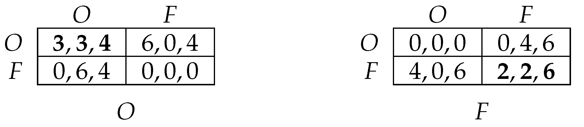
Figure 1 illustrates the battle of the sex ratio [44], a three-player version of the battle of the sexes. Two players, the row and column players, prefer opera (O) to football (F) and wish to coordinate with the matrix player. If they both coordinate with the matrix player, then they have an equal chance of accompanying the matrix player to the chosen event, and thus share the coordination payoff. The matrix player prefers football to opera and wishes to coordinate with at least one of the other players.

Let the set of individuals be $\mathcal{I}=\{1,2,3\}$ with action sets $A_i=\{O,F\}$. Let individuals $1,2,3\in \mathcal{I}$ respectively correspond to the row, column and matrix players of the game in Figure 1. For each state of the world $\omega$, let individual payoffs $u_i$ be given by the entries of the payoff matrix. Consider a state space, $\Omega =\{{\omega }_0,{\omega }_1\}$, $\Pi \left({\omega }_0\right)=\{\left\{1\right\},\left\{2\right\},\left\{3\right\}\}$, $\Pi \left({\omega }_1\right)=\{\left\{1\right\},\{2,3\}\}$. Let $P\left({\omega }_0\right)=1-p$, $P\left({\omega }_1\right)=p$; ${\mathcal{Q}}_1=\left\{\{{\omega }_0,{\omega }_1\}\right\}$, ${\mathcal{Q}}_2={\mathcal{Q}}_3=\{\left\{{\omega }_0\right\},\left\{{\omega }_1\right\}\}$.

There are three possible Pareto agency equilibria in pure strategies. For two of these equilibria to exist, the probability p that the collective agent $\{2,3\}$ is formed (i.e., the state is ${\omega }_1$) must be low enough that the actions chosen by the collective agent do not affect choices when the collective agent does not form (i.e., at state ${\omega }_0$). For $p\le \raisebox{1ex}{$3$}\!\left/ \!\raisebox{-1ex}{$5$}\right.$,

$$\begin{array}{c}{\sigma }_1\left(O\right|{\omega }_0)={\sigma }_1\left(O\right|{\omega }_1)=1,{\sigma }_2\left(O\right|{\omega }_0)=1,{\sigma }_3\left(O\right|{\omega }_0)=1,\hfill \\ {\sigma }_{\{2,3\}}\left((F,F)\right|{\omega }_1)=1,\hfill \end{array}$$

is an equilibrium, and for $p\le \raisebox{1ex}{$2$}\!\left/ \!\raisebox{-1ex}{$5$}\right.$,

$$\begin{array}{c}{\sigma }_1\left(F\right|{\omega }_0)={\sigma }_1\left(F\right|{\omega }_1)=1,{\sigma }_2\left(F\right|{\omega }_0)=1,{\sigma }_3\left(F\right|{\omega }_0)=1,\hfill \\ {\sigma }_{\{2,3\}}\left((O,O)\right|{\omega }_1)=1,\hfill \end{array}$$

is an equilibrium.

The third equilibrium exists for all $0<p<1$. This is the equilibrium at which action F is always played by every agent,

$$\begin{array}{c}{\sigma }_1\left(F\right|{\omega }_0)={\sigma }_1\left(F\right|{\omega }_1)=1,{\sigma }_2\left(F\right|{\omega }_0)=1,{\sigma }_3\left(F\right|{\omega }_0)=1,\hfill \\ {\sigma }_{\{2,3\}}\left((F,F)\right|{\omega }_1)=1.\hfill \end{array}$$

We will see below that there is no equivalent equilibrium at which action O is always played.

Pareto agency equilibria in mixed strategies also exist. For example,

$$\begin{array}{c}{\sigma }_1\left(F\right|{\omega }_0)={\sigma }_1\left(F\right|{\omega }_1)=1,{\sigma }_2\left(F\right|{\omega }_0)=1,{\sigma }_3\left(F\right|{\omega }_0)=1,\hfill \\ {\sigma }_{\{2,3\}}\left((F,F)\right|{\omega }_1)=q,{\sigma }_{\{2,3\}}\left((O,O)\right|{\omega }_1)=1-q,\hfill \end{array}$$

is an equilibrium for $q\ge 1-\raisebox{1ex}{$2$}\!\left/ \!\raisebox{-1ex}{$5p$}\right.$. For $q=0$, this reduces to the condition $p\le \raisebox{1ex}{$2$}\!\left/ \!\raisebox{-1ex}{$5$}\right.$ for the second of our pure strategy equilibria above. The expected payoff of individual 2 in this equilibrium is $2q+6(1-q)=6-4q$ (decreasing in q) and the expected payoff of individual 3 is $6q+4(1-q)=4+2q$ (increasing in q). As there is no aggregate payoff function and we deal with Pareto relations, agent $\{2,3\}$ has no preference ordering over these values of q, but this is not the same as indifference. Finally, we note that

$$\begin{array}{c}{\sigma }_1\left(O\right|{\omega }_0)={\sigma }_1\left(O\right|{\omega }_1)=1,{\sigma }_2\left(O\right|{\omega }_0)=1,{\sigma }_3\left(O\right|{\omega }_0)=1,\hfill \\ {\sigma }_{\{2,3\}}\left((F,F)\right|{\omega }_1)=q,{\sigma }_{\{2,3\}}\left((O,O)\right|{\omega }_1)=1-q,\hfill \end{array}$$

is never an equilibrium for $q<1$, the reason being that the expected payoff of individual 2 is $4q+3(1-q)=3+q$ (increasing in q) and the expected payoff of individual 3 is $6q+4(1-q)=4+2q$ (increasing in q), so all $q<1$ are Pareto dominated by $q=1$, which corresponds to the first of our pure strategy equilibria above.

4.2. Comparison of Agency Equilibrium and Pareto Agency Equilibrium

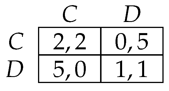
Let the set of individuals be $\mathcal{I}=\{1,2\}$ with action sets $A_i=\{C,D\}$. Let individuals $1,2\in \mathcal{I}$ respectively correspond to the row and column players of the prisoner’s dilemma game in Figure 2. For each state of the world $\omega$, let individual payoffs $u_i$ be given by the entries of the payoff matrix. Consider a state space, $\Omega =\{{\omega }_0,{\omega }_1\}$, $\Pi \left({\omega }_0\right)=\{\left\{1\right\},\left\{2\right\}\}$, $\Pi \left({\omega }_1\right)=\left\{\{1,2\}\right\}$. Let $P\left({\omega }_0\right)=1-p$, $P\left({\omega }_1\right)=p$; ${\mathcal{Q}}_1={\mathcal{Q}}_2=\{\left\{{\omega }_0\right\},\left\{{\omega }_1\right\}\}$.

Thus, the game is a prisoner’s dilemma in which the two individuals may sometimes, with probability p, constitute a single agent. At state ${\omega }_0$, the agents are individuals and play D at any agency equilibrium or Pareto agency equilibrium,

$$\begin{array}{c}{\sigma }_1\left(D\right|{\omega }_0)={\sigma }_2\left(D\right|{\omega }_0)=1.\hfill \end{array}$$

At Pareto agency equilibrium, at state ${\omega }_1$, some Pareto efficient strategy profile will be played by agent $\{1,2\}$,

$$\begin{array}{c}{\sigma }_{\{1,2\}}\left((C,D)\right|{\omega }_1)+{\sigma }_{\{1,2\}}\left((D,C)\right|{\omega }_1)=1.\hfill \end{array}$$

This completes the description of the set of Pareto agency equilibria.

For some v, the set of agency equilibria is disjoint with the set of Pareto agency equilibria, even when an agent’s payoff is strictly increasing in the payoffs of each of its constituent individuals. Consider $v_{\{1,2\}}=\sqrt{u_1}+\sqrt{u_2}$. In this case, the payoff of $\{1,2\}$ is maximized only when $(C,C)$ is played with probability one, so the unique agency equilibrium has

$$\begin{array}{c}{\sigma }_{\{1,2\}}\left((C,C)\right|{\omega }_1)=1.\hfill \end{array}$$

In contrast, if $v_{\{1,2\}}={\lambda }_1{u}_1+{\lambda }_2{u}_2$ for ${\lambda }_1,{\lambda }_2>0$, the set of agency equilibria is a subset of the set of Pareto agency equilibria. If ${\lambda }_1={\lambda }_2$, then every Pareto agency equilibrium is an agency equilibrium. If ${\lambda }_1\ne {\lambda }_2$, then there is a unique agency equilibrium with

$$\begin{array}{c}{\sigma }_{\{1,2\}}\left((C,D)\right|{\omega }_1)=1\mathrm{if}{\lambda }_1<{\lambda }_2,\hfill \\ {\sigma }_{\{1,2\}}\left((D,C)\right|{\omega }_1)=1\mathrm{if}{\lambda }_1>{\lambda }_2.\hfill \end{array}$$

These specific characterizations arise from the linearity of the Pareto frontier in this Prisoner’s dilemma. However, the general observation applies to all games: the set of agency equilibria under utilitarian payoffs is always a subset of the Pareto agency equilibria.

Proposition 1.

If σ is an agency equilibrium of $(\mathcal{U},\Pi ,v)$ and, for all $J\subseteq \mathcal{I}$, $\omega \in \Omega$, $v_J(·,\omega )={\sum }_{i\in J}{\lambda }_i{u}_i(·,\omega )$, where ${\lambda }_i$ are strictly positive welfare weights, then σ is a Pareto agency equilibrium of $(\mathcal{U},\Pi )$.

Proof. 

Assume that there exists an agency equilibrium $\sigma$ of $(\mathcal{U},\Pi ,v)$ that is not a Pareto agency equilibrium of $(\mathcal{U},\Pi )$. Therefore, by Definition 4, for some $\omega \in \Omega$, $J\in \Pi \left(\omega \right)$, there exists a Pareto deviation ${\tilde{\sigma }}_J\left(\omega \right)\in \Delta A_J$. Taking Definition 3 and summing over $i\in J$, we have

$$\begin{array}{c}\sum _{i\in J}{\lambda }_i\sum _{{\omega }^{\prime }\in Q_J\left(\omega \right)}{u}_i(\{{\tilde{\sigma }}_J\left(\omega \right),{\sigma }_{-J}\left({\omega }^{\prime }\right)\},{\omega }^{\prime })P\left[{\omega }^{\prime }\right|Q_J\left(\omega \right)]\hfill \\ >\sum _{i\in J}{\lambda }_i\sum _{{\omega }^{\prime }\in Q_J\left(\omega \right)}{u}_i(\sigma \left({\omega }^{\prime }\right),{\omega }^{\prime })P\left[{\omega }^{\prime }\right|Q_J\left(\omega \right)].\hfill \end{array}$$

Reordering the summations,

$$\begin{array}{c}\sum _{{\omega }^{\prime }\in Q_J\left(\omega \right)}\sum _{i\in J}{\lambda }_i{u}_i(\{{\tilde{\sigma }}_J\left(\omega \right),{\sigma }_{-J}\left({\omega }^{\prime }\right)\},{\omega }^{\prime })P\left[{\omega }^{\prime }\right|Q_J\left(\omega \right)]\hfill \\ >\sum _{{\omega }^{\prime }\in Q_J\left(\omega \right)}\sum _{i\in J}{\lambda }_i{u}_i(\sigma \left({\omega }^{\prime }\right),{\omega }^{\prime })P\left[{\omega }^{\prime }\right|Q_J\left(\omega \right)],\hfill \end{array}$$

we obtain

$$\begin{array}{c}\sum _{{\omega }^{\prime }\in Q_J\left(\omega \right)}{v}_J(\{{\tilde{\sigma }}_J\left(\omega \right),{\sigma }_{-J}\left({\omega }^{\prime }\right)\},{\omega }^{\prime })P\left[{\omega }^{\prime }\right|Q_J\left(\omega \right)]\hfill \\ >\sum _{{\omega }^{\prime }\in Q_J\left(\omega \right)}{v}_J(\sigma \left({\omega }^{\prime }\right),{\omega }^{\prime })P\left[{\omega }^{\prime }\right|Q_J\left(\omega \right)],\hfill \end{array}$$

and, expanding the left hand side,

$$\begin{array}{c}\sum _{{\omega }^{\prime }\in Q_J\left(\omega \right)}{\int }_{a_J\in A_J}{v}_J(\{a_J,{\sigma }_{-J}\left({\omega }^{\prime }\right)\},{\omega }^{\prime })\mathrm{d}{\tilde{\sigma }}_J\left(a_J\right|\omega )P\left[{\omega }^{\prime }\right|Q_J\left(\omega \right)]\hfill \\ >\sum _{{\omega }^{\prime }\in Q_J\left(\omega \right)}{v}_J(\sigma \left({\omega }^{\prime }\right),{\omega }^{\prime })P\left[{\omega }^{\prime }\right|Q_J\left(\omega \right)].\hfill \end{array}$$

As $v_J$ is measurable, by Fubini’s Theorem we can rearrange to get

$$\begin{array}{c}{\int }_{a_J\in A_J}\sum _{{\omega }^{\prime }\in Q_J\left(\omega \right)}{v}_J(\{a_J,{\sigma }_{-J}\left({\omega }^{\prime }\right)\},{\omega }^{\prime })P\left[{\omega }^{\prime }\right|Q_J\left(\omega \right)]\mathrm{d}{\tilde{\sigma }}_J\left(a_J\right|\omega )\hfill \\ >\sum _{{\omega }^{\prime }\in Q_J\left(\omega \right)}{v}_J(\sigma \left({\omega }^{\prime }\right),{\omega }^{\prime })P\left[{\omega }^{\prime }\right|Q_J\left(\omega \right)].\hfill \end{array}$$

The inequality implies that the integrand cannot be less than or equal to the expression on the right hand side of the inequality for every $a_J\in A_J$, so for some ${\tilde{a}}_J\in A_J$ we must have

$$\begin{array}{c}\sum _{{\omega }^{\prime }\in Q_J\left(\omega \right)}{v}_J(\{{\tilde{a}}_J,{\sigma }_{-J}\left({\omega }^{\prime }\right)\},{\omega }^{\prime })P\left[{\omega }^{\prime }\right|Q_J\left(\omega \right)]\hfill \\ >\sum _{{\omega }^{\prime }\in Q_J\left(\omega \right)}{v}_J(\sigma \left({\omega }^{\prime }\right),{\omega }^{\prime })P\left[{\omega }^{\prime }\right|Q_J\left(\omega \right)],\hfill \end{array}$$

which, by Definition 1, is the condition for ${\tilde{a}}_J$ to be a profitable deviation. Therefore, by Definition 2, $\sigma$ is not an agency equilibrium of $(\mathcal{U},\Pi ,v)$. Contradiction. □

Proposition 1 can be used to derive an existence theorem for Pareto agency equilibrium. The finiteness conditions that Theorem 1 places on $\mathcal{U}$ are independent of v. Under these conditions, the set of agency equilibria of $(\mathcal{U},\Pi ,v)$ is nonempty for any v, so it is nonempty for utilitarian v. By Proposition 1, this nonempty set is a subset of the set of Pareto agency equilibria of $(\mathcal{U},\Pi )$, which is thus also nonempty.

Theorem 2.

If $\mathcal{U}$ is such that Ω, $A_i$, $i\in \mathcal{I}$ are finite, then the set of Pareto agency equilibria of $(\mathcal{U},\Pi )$ is nonempty.

Proof. 

For all $J\subseteq \mathcal{I}$, let $v_J(·,\omega )={\sum }_{i\in J}{\lambda }_i{u}_i(·,\omega )$, where ${\lambda }_i$ are strictly positive welfare weights. By Theorem 1, the set of agency equilibria of $(\mathcal{U},\Pi ,v)$ is nonempty. By Proposition 1, the set of agency equilibria of $(\mathcal{U},\Pi ,v)$ is a subset of the set of Pareto agency equilibria of $(\mathcal{U},\Pi )$, which is therefore also nonempty. □

In the example of the Prisoner’s dilemma of Figure 2, we saw that a specific utilitarian v with ${\lambda }_1={\lambda }_2$ made every Pareto agency equilibrium of $(\mathcal{U},\Pi )$ an agency equilibrium of $(\mathcal{U},\Pi ,v)$. In general, such a choice of weights ${\lambda }_1$, ${\lambda }_2$ is not possible, as we can see by amending the payoffs of the prisoner’s dilemma in Figure 2 so that $u_1\left((C,C)\right)=u_2\left((C,C)\right)=3$. This creates a kink in the Pareto frontier such that no choice of ${\lambda }_1$, ${\lambda }_2$ will lead to points on both sides of the kink maximizing v.

However, any given Pareto agency equilibrium can be supported as an agency equilibrium for some utilitarian v with state-dependent ${\lambda }_i\left(\omega \right)$. State dependence is required to account for the possibility that a given Pareto agency equilibrium involves some agent J playing different Pareto efficient action subprofiles at different states.

Proposition 2.

If σ is a Pareto agency equilibrium of $(\mathcal{U},\Pi )$, then there exist $v_J(·,\omega )={\sum }_{i\in J}{\lambda }_i\left(\omega \right)u_i(·,\omega )$, $J\subseteq \mathcal{I}$, $\omega \in \Omega$, ${\lambda }_i\left(\omega \right)\ge 0$, such that σ is an agency equilibrium of $(\mathcal{U},\Pi ,v)$.

Proof. 

For given $\omega$, $J\in \Pi \left(\omega \right)$, consider ${\sigma }_J^1,{\sigma }_J^2\in \Delta A_J$. If ${\alpha }^1,{\alpha }^2\in {\mathbb{R}}_{+}$, ${\alpha }^1+{\alpha }^2=1$, ${\tilde{\sigma }}_J={\alpha }^1{\sigma }_J^1+{\alpha }^2{\sigma }_J^2$, then ${\tilde{\sigma }}_J\in \Delta A_J$. As all measures have domain $A_J$ and $u_i$ is ${\Delta }_J$-measurable, the integral over the sum of measures that defines $u_i$ given the mixed strategy ${\tilde{\sigma }}_J={\sigma }_J^1+{\sigma }_J^2$ is equal to the sum of integrals over those measures (see, e.g., [52]), and we obtain the following expression linking the expected payoffs of $i\in J$ under ${\tilde{\sigma }}_J\left(\omega \right)$, ${\sigma }_J^1\left(\omega \right)$ and ${\sigma }_J^2\left(\omega \right)$, taking ${\sigma }_{-J}$ and $\omega$ as given.

$$\begin{array}{c}\sum _{{\omega }^{\prime }\in Q_J\left(\omega \right)}{u}_i(\{{\tilde{\sigma }}_J\left(\omega \right),{\sigma }_{-J}\left({\omega }^{\prime }\right)\},{\omega }^{\prime })P\left[{\omega }^{\prime }\right|Q_J\left(\omega \right)]\hfill \\ ={\alpha }^1\sum _{{\omega }^{\prime }\in Q_J\left(\omega \right)}{u}_i(\{{\sigma }_J^1\left(\omega \right),{\sigma }_{-J}\left({\omega }^{\prime }\right)\},{\omega }^{\prime })P\left[{\omega }^{\prime }\right|Q_J\left(\omega \right)]\hfill \\ +{\alpha }^2\sum _{{\omega }^{\prime }\in Q_J\left(\omega \right)}{u}_i(\{{\sigma }_J^2\left(\omega \right),{\sigma }_{-J}\left({\omega }^{\prime }\right)\},{\omega }^{\prime })P\left[{\omega }^{\prime }\right|Q_J\left(\omega \right)].\hfill \end{array}$$

So the set of feasible expected payoff vectors for J, given ${\sigma }_{-J}$ and $\omega$, is a convex set in ${\mathbb{R}}^J$. Denote this set $\mathbf{U}$.

Let $\sigma (·)={\left({\sigma }_J(·)\right)}_{J\in \Pi (·)}$ be a Pareto agency equilibrium of $(\mathcal{U},\Pi )$. Let $U_J\in {\mathbb{R}}^J$ be the vector of expected payoffs at state $\omega$ of players in $J\in \Pi \left(\omega \right)$ at this equilibrium. That is, $U_J={\left(U_i\right)}_{i\in J}$ and

$$\begin{array}{c}{U}_i:=\sum _{{\omega }^{\prime }\in Q_J\left(\omega \right)}{u}_i(\sigma \left({\omega }^{\prime }\right),{\omega }^{\prime })P\left[{\omega }^{\prime }\right|Q_J\left(\omega \right)],i\in J.\hfill \end{array}$$

As $\sigma$ is a Pareto agency equilibrium and $J\in \Pi \left(\omega \right)$, $\mathbf{U}$ does not contain any payoff vectors that Pareto dominate $U_J$. Moreover, $\mathbf{D}$, the set of payoff vectors that Pareto dominate $U_J$, is a convex set. By the Separating Hyperplane Theorem, we can choose a hyperplane $f\left({\left(x_i\right)}_{i\in J}\right)=0$ in ${\mathbb{R}}^J$ that separates $\mathbf{U}$ and $\mathbf{D}$. This plane intersects $U_J$. Let $\nabla f$ be the gradient vector of f, which is constant as $f=0$ is a hyperplane. Either $(U_J+\nabla f)\in \mathbf{D}$, in which case, by definition of $\mathbf{D}$, $\nabla f$ is non-negative, or $(U_J-\nabla f)\in \mathbf{D}$, in which case $-\nabla f$ is non-negative.

Let ${\lambda }_i\left(\omega \right)=\left|{(\nabla f)}_i\right|$, $i\in J$, and $v_J(·,\omega )={\sum }_{i\in J}{\lambda }_i\left(\omega \right)u_i(·,\omega )$. The indifference curves of $v_J(·,\omega )$ in terms of ${\left\{u_i(·,\omega )\right\}}_{i\in J}$ are then given by $f\left({\left(x_i\right)}_{i\in J}\right)=k$, for $k\in \mathbb{R}$, and $v_J(·,\omega )$ attains its maximum value in $\mathbf{U}$ at ${\sigma }_J\left(\omega \right)$. Hence, if $v_J$ is defined in this way for all $\omega$, $J\in \Pi \left(\omega \right)$, then $\sigma$ is an agency equilibrium of $(\mathcal{U},\Pi ,v)$. □

5. Discussion

This paper has presented two fixed-point solution concepts, agency equilibrium and Pareto agency equilibrium, that allow for multiple levels of agency with potentially conflicting incentives. One of these concepts, agency equilibrium, involves the specification of payoffs for collective agents. The other concept, Pareto agency equilibrium, relies on Pareto dominance arguments and does not specify any additional payoffs beyond those of individuals. The model and both concepts should be readily accessible to anyone with a basic knowledge of games of incomplete information. Moreover, the ideas are easily teachable and applicable to any game theoretic situation in which collective agency is a possibility.

Readers may have a preference for one of the solution concepts over the other. In prior work on adaptive dynamics (see Remark 9), the author has emphasized the advantages of making a clear conceptual distinction between agency and payoffs. Pareto agency equilibrium does this, defining payoffs at the level of the individual while allowing multiple levels of agency. However, as long as choice by an agent is consistent with the usual axioms, it will be representable by a payoff function at the level of the agent itself. This is the approach taken by agency equilibrium, which adds some flexibility in that it allows for collective payoffs that are misaligned with individual payoffs, such as when Alice and Bob each individually prefer action profile $a^{\prime }$ to profile $a^{″}$, but as a collective prefer profile $a^{″}$ to $a^{\prime }$. In any case, as we saw in Section 4.2, it is instructive to consider each of these concepts with reference to the other.

References

- Heath, J. Methodological individualism. In The Stanford Encyclopedia of Philosophy; Zalta, E.N., Ed.; Metaphysics Research Lab, Stanford University: Stanford, CA, USA, 2015. [Google Scholar]
- Schumpeter, J. On the concept of social value. Q. J. Econ. 1909, 23, 213–232. [Google Scholar] [CrossRef]
- Weber, M. Wirtschaft und Gesellschaft: Grundriss der Verstehenden Soziologie; Mohr Siebeck: Heidelberg, Germany, 1922. [Google Scholar]
- Arrow, K.J. Methodological individualism and social knowledge. Am. Econ. Rev. 1994, 84, 1–9. [Google Scholar]
- Samuelson, L. Game theory in economics and beyond. J. Econ. Perspect. 2016, 30, 107–130. [Google Scholar] [CrossRef]
- Friedman, M. Essays in Positive Economics; University of Chicago Press: Chicago, IL, USA, 1953. [Google Scholar]
- Keynes, J.N. The Scope and Method of Political Economy, 1st ed.; Routledge, Taylor and Francis e-books: London, UK, 1890. [Google Scholar]
- Searle, J. Collective intentions and actions. In Intentions in Communication; Cohen, P.R., Morgan, J., Pollack, M., Eds.; MIT Press: Cambridge, MA, USA, 1990; pp. 401–415. [Google Scholar]
- Tomasello, M. A Natural History of Human Thinking; Harvard University Press: Cambridge, MA, USA, 2014. [Google Scholar]
- Tuomela, R.; Miller, K. We-intentions. Philos. Stud. 1988, 53, 367–389. [Google Scholar] [CrossRef]
- Angus, S.D.; Newton, J. Emergence of shared intentionality is coupled to the advance of cumulative culture. PLoS Comput. Biol. 2015, 11, e1004587. [Google Scholar] [CrossRef]
- Newton, J. Shared intentions: The evolution of collaboration. Games Econ. Behav. 2017, 104, 517–534. [Google Scholar] [CrossRef]
- Kuhn, S. Prisoner’s dilemma. In The Stanford Encyclopedia of Philosophy; Zalta, E.N., Ed.; Metaphysics Research Lab, Stanford University: Stanford, CA, USA, 2014. [Google Scholar]
- Hardin, G. The tragedy of the commons. Science 1968, 162, 1243–1248. [Google Scholar]
- Lloyd, W.F. Two Lectures on the Checks to Population; S. Collingwood, Oxford: Oxford, England, UK, 1833. [Google Scholar]
- Harsanyi, J.C. Games with incomplete information played by “bayesian” players, i-iii. part i. the basic model. Manag. Sci. 1967, 14, 159–182. [Google Scholar] [CrossRef]
- Harsanyi, J.C. Games with incomplete information played by “bayesian” players part ii. bayesian equilibrium points. Manag. Sci. 1968, 14, 320–334. [Google Scholar] [CrossRef]
- Harsanyi, J.C. Games with incomplete information played by ‘bayesian’ players, part iii. the basic probability distribution of the game. Manag. Sci. 1968, 14, 486–502. [Google Scholar] [CrossRef]
- Biran, O.; Forges, F. Core-stable rings in auctions with independent private values. Games Econ. Behav. 2011, 73, 52–64. [Google Scholar] [CrossRef]
- Ray, D.; Vohra, R. Equilibrium binding agreements. J. Econ. Theory 1997, 73, 30–78. [Google Scholar] [CrossRef]
- Ray, D. A Game-Theoretic Perspective on Coalition Formation; Oxford University Press: Oxford, UK, 2007. [Google Scholar]
- Lewis, D. Convention: A Philosophical Study; Harvard University Press: Cambridge, MA, USA, 1969. [Google Scholar]
- Schelling, T.C. The Strategy of Conflict; Reprint 1980; Harvard University Press: Cambridge, MA, USA, 1960. [Google Scholar]
- Kajii, A.; Morris, S. The robustness of equilibria to incomplete information. Econometrica 1997, 65, 1283–1309. [Google Scholar] [CrossRef]
- Bacharach, M. Interactive team reasoning: A contribution to the theory of cooperation. Res. Econ. 1999, 53, 117–147. [Google Scholar] [CrossRef]
- Bacharach, M. Beyond Individual Choice: Teams and Frames in Game Theory; Princeton University Press: Princeton, NJ, USA, 2006. [Google Scholar]
- Lecouteux, G. What does “we” want? team reasoning, game theory, and unselfish behaviours. Revue d’´economie Politique 2018, 128, 311–332. [Google Scholar] [CrossRef]
- Sugden, R. Thinking as a team: Towards an explanation of nonselfish behavior. Soc. Philos. Policy 1993, 10, 69–89. [Google Scholar] [CrossRef]
- Sugden, R. The logic of team reasoning. Philos. Explor. 2003, 6, 165–181. [Google Scholar] [CrossRef]
- Gold, N.; Sugden, R. Collective intentions and team agency. J. Philos. 2007, 104, 109–137. [Google Scholar] [CrossRef]
- Allen, B. Incentives in market games with asymmetric information: the core. Econ. Theory 2003, 21, 527–544. [Google Scholar] [CrossRef]
- Forges, F.; Minelli, E. A note on the incentive compatible core. J. Econ. Theory 2001, 98, 179–188. [Google Scholar] [CrossRef]
- Forges, F.; Minelli, E.; Vohra, R. Incentives and the core of an exchange economy: A survey. J. Math. Econ. 2002, 38, 1–41. [Google Scholar] [CrossRef]
- Vohra, R. Incomplete information, incentive compatibility, and the core. J. Econ. Theory 1999, 86, 123–147. [Google Scholar] [CrossRef]
- Wilson, R. Information, efficiency, and the core of an economy. Econometrica 1978, 46, 807–816. [Google Scholar] [CrossRef]
- Forges, F.; Serrano, R. Cooperative games with incomplete information: Some open problems. Int. Game Theory Rev. 2013, 15, 1340009. [Google Scholar] [CrossRef]
- Nozick, R. The Nature of Rationality; Princeton University Press: Princeton, NJ, USA, 1994. [Google Scholar]
- Aumann, R. Acceptable points in general cooperative n-person games. In Contributions to the Theory of Games IV; Tucker, A.W., Luce, R.D., Eds.; Princeton University Press: Princeton, NJ, USA, 1959; pp. 287–324. [Google Scholar]
- Ichiishi, T.; Idzik, A. Bayesian cooperative choice of strategies. Int. J. Game Theory 1996, 25, 455–473. [Google Scholar] [CrossRef]
- Bernheim, B.D.; Peleg, B.; Whinston, M.D. Coalition-proof Nash equilibria i. concepts. J. Econ. Theory 1987, 42, 1–12. [Google Scholar] [CrossRef]
- Moreno, D.; Wooders, J. Coalition-proof equilibrium. Games Econ. Behav. 1996, 17, 80–112. [Google Scholar] [CrossRef]
- Feldman, A.M. Recontracting stability. Econometrica 1974, 42, 35–44. [Google Scholar] [CrossRef]
- Green, J.R. The stability of Edgeworth’s recontracting process. Econometrica 1974, 42, 21–34. [Google Scholar] [CrossRef]
- Nax, H.H.; Pradelski, B.S.R. Evolutionary dynamics and equitable core selection in assignment games. Int. J. Game Theory 2015, 44, 903–932. [Google Scholar] [CrossRef]
- Newton, J. Coalitional stochastic stability. Games Econ. Behav. 2012, 75, 842–854. [Google Scholar] [CrossRef]
- Newton, J. Recontracting and stochastic stability in cooperative games. J. Econ. Theory 2012, 147, 364–381. [Google Scholar] [CrossRef]
- Newton, J.; Angus, S.D. Coalitions, tipping points and the speed of evolution. J. Econ. Theory 2015, 157, 172–187. [Google Scholar] [CrossRef]
- Newton, J.; Sawa, R. A one-shot deviation principle for stability in matching problems. J. Econ. Theory 2015, 157, 1–27. [Google Scholar] [CrossRef]
- Roth, A.E.; Vande Vate, J.H. Random paths to stability in two-sided matching. Econometrica 1990, 58, 1475–1480. [Google Scholar] [CrossRef]
- Nash, J. Non-cooperative games. Ann. Math. 1951, 54, 286–295. [Google Scholar] [CrossRef]
- Cournot, A.A. Recherches sur les principes math´ematiques de la th´eorie des richesses par Augustin Cournot; chez L. Hachette: Paris, France, 1838. [Google Scholar]
- Fremlin, D.H. Measure Theory: Broad Foundations; Torres Fremlin: Colchester, England, UK, 2001. [Google Scholar]