Abstract
We propose a model in which agents of a population interacting according to a network of contacts play games of coordination with each other and can also dynamically break and redirect links to neighbors if they are unsatisfied. As a result, there is co-evolution of strategies in the population and of the graph that represents the network of contacts. We apply the model to the class of pure and general coordination games. For pure coordination games, the networks co-evolve towards the polarization of different strategies. In the case of general coordination games our results show that the possibility of refusing neighbors and choosing different partners increases the success rate of the Pareto-dominant equilibrium.
1. Introduction
The purpose of Game Theory [1] is to describe situations in which two or more agents or entities may pursue different views about what is to be considered best by each of them. In other words, Game Theory, or at least the non-cooperative part of it, strives to describe what the agents’ rational decisions should be in such conflicting situations. For example, games such as the well known Prisoner’s Dilemma have been heavily used in order to represent the tension that appears in society when individual objectives are in conflict with socially desirable outcomes. Indeed, a large part of the research literature has focused on conflicting situations in order to uncover the mechanisms that could lead to cooperation instead of socially harmful outcomes (see e.g., [2] for a synthesis). However, there are important situations in society that do not require players to use aggressive strategies. In fact, many frequent social and economic activities require individuals to coordinate their actions on a common goal since in many cases the best course of action is to conform to the standard behavior. For example, if someone’s native language is French and she travels to an English-speaking country, it pays off to follow the local norm, i.e., to speak English instead of French. Games that express this extremely common kind of interactions are called coordination games.
Coordination games confront the players with multiple Nash equilibria and the consequent problem of how to choose among them. A useful approach has been to turn to evolutionary and learning ideas which offer a dynamical perspective based on the forces of biological and social evolution. In evolutionary game theory (EGT), the concept of a population of players where strategies that score best are more likely to be selected and reproduced provides a justification for the appearance of stable states of the dynamics that represent solutions of the game [1,3].
For mathematical convenience, standard EGT is based on infinite mixing populations where pairs of individuals are drawn uniformly at random at each step and play the game. Correlations are absent by definition and the population has an homogeneous structure. However, everyday observation tells us that in animal and human societies, individuals usually tend to interact more often with some specified subset of partners; for instance, teenagers tend to adopt the fashions of their close friends group; closely connected groups usually follow the same religion, and so on. Likewise, in the economic world, a group of firms might be directly connected because they share capital, technology, or otherwise interact in some way. In short, social interaction is mediated by networks, in which vertices identify people, firms etc., and edges identify some kind of relation between the concerned vertices such as friendship, collaboration, and economic exchange. Thus, locality of interaction plays an important role. This kind of approach was pioneered in EGT by Nowak and May [4] by using simple two-dimensional regular grids. Recently, in the wake of a surge of activity in network research in many fields [5], the dynamical and evolutionary behavior of games on networks that are more likely to represent actual social interactions than regular grids has been investigated (see [6] for a comprehensive recent review). These studies have shown that there are network structures, such as scale-free and actual social networks that may favor the emergence of cooperation with respect to the fully mixing populations used in the theory [7,8]. Most studies have focused on conflicting games but some work has also been done on games of the coordination type [8,9,10].
However, the above approach assumes a static point of view, i.e., it takes the network of contacts as being fixed once and for all and investigates the evolution of the agents’ strategies over time. In other words, it is as if we took a snapshot of a given network at a given time and used this situation during all future times. Actually, however, social networks are dynamical entities that change constantly: actors may join and leave networks at unpredictable times and they may accumulate and abandon ties over time. Using static networks is a useful first approximation however, especially for the cases where the rate of change of the network structure is slow with respect to the rate of change of individual’s behaviors. This could be the case of long-term collaboration networks, friendship, or of biological networks that are the result of an extremely long and slow evolution. But in many cases this static picture does not fit the reality very well. If we think of social or pseudo-social networks such as e-mail exchanges, Facebook-like networks, rumor-spreading networks and a host of other similar structures, we see that the evolution of the network of contacts itself can be quite rapid and plays an important role.
In the present work we study the co-evolution of agents’ behavior and of the agents’ ties in the network over time. For the sake of simplicity, we investigate constant-size systems, i.e., we start with a finite-size network of agents and allow agents to abandon and to create links among themselves but there will be no new agents joining the system, nor agents will be allowed to leave it. This is not what happens in actual social and technological networks, which all tend to grow with time and are actually non-equilibrium systems, but our “closed system” approximation is simpler to simulate and interpret, and will allow us to already draw significant conclusions. Our methodology is essentially computer simulation-based since complex networks inhomogeneity and correlations make standard mean-field methods not adequate.
Some previous work has been done on evolutionary games on dynamic networks essentially dealing with the Prisoner’s Dilemma, (e.g., [9,11,12,13]) and a recent review of these approaches has been written by Perc and Szolnoki [14]. The present study follows our own model described in [15,16] which differs from other approaches in the way in which links between agents are represented and interpreted, as explained later. In these previous works we studied the antagonistic Hawk Doves game and the Prisoner’s Dilemma with replicator dynamics, instead of the best response dynamics used here for coordination games.
We also note that in the last fifteen years economists have put forward a theory of strategic network formation, i.e., formal models of how utility-based link formation moves might be implemented in order to reach a Nash equilibrium for all the members of the network (see e.g., Jackson’s book for a synthesis of this work [17]). Our approach is different from the above view of strategic network formation for two reasons. First, we use networks that are at least two orders of magnitude larger and, while the equilibrium predictions resulting from strategic considerations usually lead to very simple topological structures such as small cliques or stars, our large evolving networks show complex structure and behavior. Second, while in strategic network formation the evolution of the network is submitted to utility maximization on the part of the players, our linking moves are based on very simple forms of reinforcement learning. Only the decisions of players concerning their behavioral strategies are based on a formal game payoff matrix.
The paper is organized as follows. In the next section we present a brief introduction to the subject of coordination games, in order to make the work self-contained. Then we describe the dynamical network model in Section 3. Next, in Section 4 we present and discuss the simulation results for pure coordination games. This is followed by the results on general coordination games in Section 5. Finally, in Section 6 we give our conclusions.
2. Coordination Games
2.1. General Coordination Games
General two-person, two strategies coordination games have the normal form of Table 1. With and , and are both Nash equilibria. Now, if we assume that and then is the risk-dominant equilibrium, while is the Pareto-dominant one. This simply means that players get a higher payoff by coordinating on but they risk less by using strategy β instead. There is also a third equilibrium in mixed strategies but it is evolutionarily unstable.

Table 1.
A general two-person, two strategies coordination game.
| α | ||
A well known example of games of this type are the so-called Stag Hunt games [9]. This class of games has been extensively studied analytically in an evolutionary setting [18,19] and by numerical simulation on several static model network types [8,9,10]. In the following, we shall first deal with the easier case of pure coordination games which, in spite of their simplicity, already clearly pose the equilibrium selection problem. Then we shall report results on Stag Hunt games which are more interesting in social terms as they pose a problem of “trust”, since the socially efficient solution is more risky.
2.2. Pure Coordination Games
Two-person pure coordination games have the normal form depicted in Table 2, with , and , where k is the number of strategies available to each player in the strategy set , and the u’s are payoffs. So all the Nash equilibria in pure strategies correspond to diagonal elements in the table where the two players coordinate on the same strategy, while there is a common lower uniform payoff for all other strategy pairs which is set to 0 here.
Table 2.
A general payoff bi-matrix of a two-person pure coordination game. Nash equilibria in pure strategies are marked in bold.
| … | ||||
| … | ||||
| … | … | … | … | … |
In this paper we shall consider two-person, two-strategies pure coordination games with the payoff matrix of Table 3 with . When , strategy α is said to be dominant since a player obtains a higher payoff playing α rather than β.
Table 3.
A general two-person, two-strategies pure coordination game.
| α | ||
3. Model Description
In this section we provide nomenclature and definitions for the graphs representing the population and for the dynamical decision processes implemented by the agents. The dynamical model has originally appeared in [15,16]; it is summarized here to make the paper self-contained. The network of players is represented by a directed weighted graph , where the set of vertices V represents the agents, while the set of oriented edges (or links) E represents their unsymmetric weighted interactions. The population size N is the cardinality of V. A neighbor of an agent i is any other agent j such that there is a pair of oriented edges and . The set of neighbors of i is called . For network structure description purposes, we shall also use an unoriented version of G having exactly the same set of vertices V but only a single unoriented unweighted edge between any pair of connected vertices i and j of G. For we shall define the degree of vertex as the number of neighbors of i. The average degree of the network will be called .
Each link in G has a weight or “force” that represents in an indirect way the “trust” player i places in player j. This weight may take any value in and its variation is dictated by the payoff earned by i in each encounter with j. The detailed way in which weights evolve dynamically is explained below. We define a quantity called satisfaction of an agent i as the mean weight of i’s links:
with . The link strengths can be seen as a kind of accumulated “memory” of previous encounters. However, it must be distinguished from the memory used in iterated games, in which players “remember” a certain number of previous moves and can thus conform their future strategy on the analysis of those past encounters [1,3]. Our interactions are strictly one-shot, i.e., players “forget” the strategies used by neighbors in previous rounds and cannot recognize their playing patterns over time. However, they do recognize neighbors in terms of the strengths of the links they maintain with them. It could also be useful to model progressive obsolescence of the over time, i.e., a discount rate of their values but, for the sake of simplicity, we prefer not to consider this effect in a first step.
Since we shall adopt an evolutionary approach, we must next define the decision rule by which individuals update their strategy and their contacts during time. For the strategy update, an easy and well known adaptive learning rule is myopic best-response dynamics, which embodies a primitive form of bounded rationality and for which rigorous results for coordination games are known in well mixed populations [18,20] and in fixed one-dimensional and two-dimensional lattices [19,21].
In the local version of this model, time is discrete i.e., and, in each time step, an agent has the opportunity of revising her current strategy. She does so by considering the current actions of her neighbors and switching to the action that would maximize her payoff if the neighbors would stick to their current choices. This rule is called myopic because the agents only care about immediate payoff, they cannot see far into the future. The model is thus completely local and an agent only needs to know her own current strategy, the game payoff matrix, who are her neighbors, and their current strategies. Furthermore, the agent must be able to “ask” one of her neighbors to introduce to her one of his neighbors. Given the network structure of the population, the strategy update rule is implemented as follows:
- player i will choose the action that maximizes her payoff, given that the strategy profile of her neighbors remains the same as in the previous period;
- if there is a tie or i is not given the opportunity of revising her strategy, then i will keep her current strategy.
Now we describe the dynamics of links. The active agent i will, with probability q, attempt to dismiss an interaction with one of her neighbors, say j, selected proportionally to , i.e., the higher , the lower the probability of the link being selected for rewiring. Likewise, the lower the satisfaction of agent i, the higher the probability of dismissing the link. However, although i may take the lead in the decision to dismiss a link, j has some power in opposing herself. The idea is that, in real social situations, it is seldom possible to take unilateral decisions: often there is a cost associated, and we represent this hidden cost by a probability with which j may refuse to be cut away. In other words, the link is less likely to be deleted when j’s trust in i, , is high. If the decision is finally taken to cut the link, i attempts to create a new link with a neighbor l of one of her neighbors , such that links and with high forces are probabilistically favored. Link simply disappears, as relations in the weighted graph G are always reciprocal, although the corresponding weights will, in general, be different. This process is schematically depicted in Figure 1. This process requires that agent k “introduces” one of its neighbors, say l, to i. Obviously, this bias will cause the clustering coefficient of the network to increase over time due to the transitive closure it causes, i.e., triangles will be more likely in the evolving graph. The solution adopted here is inspired by the observation that, in social networks, links are usually created more easily between people who have a satisfactory mutual acquaintance than those who do not. If the new link already exists, the process is repeated with l’s neighbors. If this also fails, a new link between i and a randomly chosen node is created. In all cases the new link is initialized with a strength of in both directions.

Figure 1.
Illustration of the rewiring of link to . Agent k is chosen to introduce player l to i (see text). Between any pair of connected agents there are two directed links: only one of them is shown for clarity.
Once the agents have played with their neighbors, and have gone through their strategy or link update steps, the strengths of the links are updated in the following way:
where is the payoff of i when interacting with j, is the payoff that i would have earned against j, if j were to play his other strategy, and () is the maximal (minimal) possible payoff obtainable in a single interaction. is the number of i’s neighbors, i.e., its degree. If falls outside the interval then it is reset to 0 if it is negative, and to 1 if it is larger than 1. This update is performed in both directions, i.e., both and are updated because both i and j get a payoff out of their encounter.
In summary, calling the population graph at time t, where each node is labeled with its present strategy and where V is fixed but evolves, the resulting stochastic process is a Markov chain since the probability of state only depends on the previous step: .
At this point, we should mention that Skyrms and coworkers [9,22] have proposed a representation of agents’ interaction based on evolvable interaction probabilities which is conceptually similar to ours, but the context is very different. Populations are small (ten players) and the network structure is never made explicit as the authors prefer to think in terms of probabilistic “encounters” instead of using the link concept. This approach allows Skyrms and coworkers to establish quantitative models based on stochastic processes for the simplest cases but it does not lead to an explicit description of the actual evolving networks. In addition, when players update their strategies, they have global knowledge of the strategy distribution of the whole population, while in our model this knowledge is strictly local.
4. Simulation Results for Pure Coordination Games
4.1. Simulation Settings
The constant size of the network during the simulations is . The initial graph is generated randomly with a mean degree . The companion oriented graph is trivially built from and forces between any pair of neighboring players are initialized at .
The non-zero diagonal payoff a has been varied in the range in steps of with ; the range is symmetrically equivalent. Each value in the phase space reported in the following figures is the average of 50 independent runs and each run has been performed on a fresh realization of the corresponding initial random graph.
To detect steady states of the dynamics 2, i.e., those states with little or no fluctuation over extended periods of time, we first let the system evolve for a transient period of times steps ( time steps when ). After a quasi-equilibrium state is reached past the transient, averages are calculated during additional time steps. A steady state has always been reached in all simulations performed within the prescribed amount of time, for most of them well before the limit.
We have experimented with different proportions of uniformly randomly distributed initial strategies α belonging to the set .
4.2. Discussion of Results
Figure 2 reports the amount of α-strategists in the population when a quasi-equilibrium state has been reached as a function of the rewiring frequency q. The upper light part of the plots indicate the region of the parameters space where the α-strategists are able to completely take over the population. This can happen because α strategy offers the best payoff since is positive, therefore β-strategists are prone to adapt in order to improve their wealth. Figure 2(a) shows the case where both α and β strategies are present in the same ratio at the beginning of the simulation. The darker region indicates the situations where diversity is able to resist. This clearly happens when the payoff difference is zero. In this case both α and β are winning strategies and the players tends to organize in two big clusters to minimize the links with the opposing faction. More surprisingly, even when one of the two strategies has a payoff advantage, the evolution of the topology of the interaction allows the less favorable strategy to resist. The faster the network evolution is (larger q), the greater the payoff difference that can be tolerated by the agents.
In Figure 2(b) the case when α represent only of the initial population is presented. When no noise is present the stronger strategy needs an increased payoff advantage to take over the population. When the payoff-inferior strategy β is able to maintain the majority.
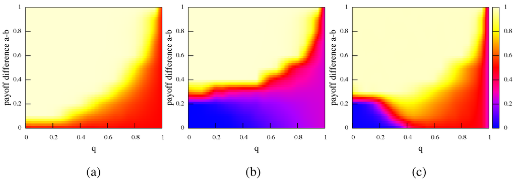
Figure 2.
Fraction of α-strategists in the population as a function of the relinking probability q when the quasi-equilibrium has been reached. (a) shows the case where the initial fraction of α is 0.5 and noise is not present. In (b) and (c) the initial fraction of α is 0.25. (b) shows the noiseless case and (c) the case where noise is 0.01. Results are averages over 50 independent runs.
To confirm the stochastic stability of the evolution process we did a series of simulations using a noisy version of the strategy evolution rule [18]. The amount of noise used is 0.01, which means that an agent will pick the wrong strategy once every 100 updates on average. This quantity is rather small and does not change the results obtained when the two populations are equally represented in the initial network, the graphic representation is almost the same of the one in Figure 2(a) with respect to stochastic fluctuations. However, when the initial share is not the same, the presence of noise allows a considerable increase in the performance of the Pareto-superior strategy when this strategy is less represented in the beginning. Figure 2(c) shows the case when the initial ratio of α-strategists is of the population. We can clearly see that the strategy that offers the higher payoff (α in this case but the results for β would obviously be symmetrical) can recover a considerable amount of the parameters space even when it starts from an unfavorable situation. The coexistence of stochastic errors and network plasticity allows the more advantageous strategy to improve its share. In this case, when the situation is almost the same as when the initial shares are the same. The same phenomenons happen when the initial ratio of α is smaller. The case of an initial ratio of has been verified but is not shown here.
For visualization purposes, Figure 3 and Figure 4 show one typical instance of the evolution of the network and of the strategy distribution from the initial state in which strategies are distributed uniformly at random to a final quasi-equilibrium steady state for a smaller network. In spite of the relatively small size, the phenomena are qualitatively the same for and , the major difference is just the time to convergence which is much shorter for .
These results have been obtained for a symmetric payoff of the strategies and for an equal initial fraction of α-strategists and β-strategists. It is visually clear that the system goes from a random state of both the network and the strategy distribution to a final one in which the network is no longer completely random and, even more important, the strategies are distributed in a completely polarized way. In other words, the system evolves toward an equilibrium where individuals following the same convention are clustered together. Since both norms are equivalent in the sense that their respective payoffs are the
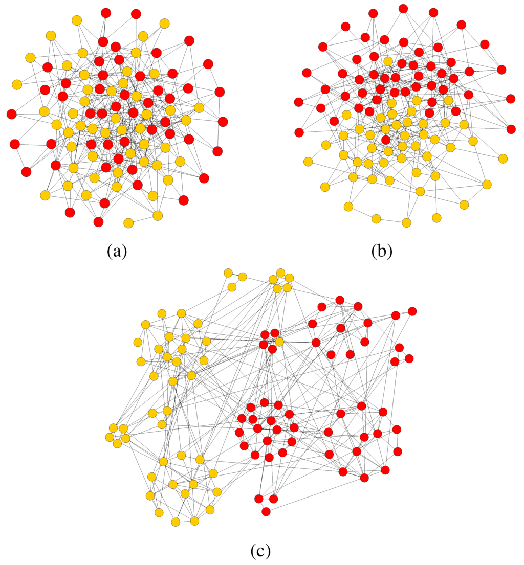 same, agents tend to pair-up with other agents playing the same strategy since playing the opposite one is a dominated strategy. The process of polarization and, in some cases, even the splitting of the graph into two distinct connected components of different colors, is facilitated by the possibility of breaking and forming links when an interaction is judged unsatisfactory by an agent. Even with a relatively small rewiring frequency of as for the case represented in the figures, polarization is reached relatively quickly. In fact, since our graphs G and are purely relational entities devoid of any metric structure, breaking a link and forming another one may also be interpreted as “moving away”, which is what would physically happen in certain social contexts. If, on the other hand, the environment is say, belonging to one of two forums on the Internet, then link rewiring would not represent any physical reconfiguration of the agents, just a different web connection. Although our model is an abstract one and does not claim any social realism, still one could imagine how conceptually similar phenomena may take place in society. For example, the two norms might represent two different dress codes. People dressing in a certain way, if they go to a public place, say a bar or a concert in which individuals dress in the other way in the majority, will tend to change place in order to feel more adapted to their surroundings. Of course, one can find many other examples that would fit this description. An early model capable of qualitatively represent this kind of phenomena was Schelling’s segregation cellular automaton [23] which was based on a simple majority rule. However, Schelling’s model, being based on a two-dimensional grid, is not realistic as a social network. Furthermore, the game theory approach allows to adjust the payoffs for a given strategy and is analytically solvable for homogeneous or regular graphs.
Figure 3.
(a) The simulation starts from a random network with and 50 players for each type. (b) In the first short part of the simulation ( time steps) the strategies reach an equilibrium, the network however is still unorganized. (c) The community structure starts then to emerge, many small clusters with nearly uniform strategy appears.
The above qualitative observations can be rendered more statistically rigorous by using the concept of communities. Communities or clusters in networks can be loosely defined as being groups of nodes that are strongly connected between them and poorly connected with the rest of the graph. These structures are extremely important in social networks and may determine to a large extent the properties of dynamical processes such as diffusion, search, and rumor spreading among others. Several methods have been proposed to uncover the clusters present in a network (for a recent review see, for instance, [24]). To detect communities, here we have used the divisive method of Girvan and Newman [25] which is based on iteratively removing edges with a high value of edge betweenness. A commonly used statistical indicator of the presence of a recognizable community structure is the modularity Q. According to Newman [26] modularity is proportional to the number of edges falling within clusters minus the expected number in an equivalent network with edges placed at random. In general, networks with strong community structure tend to have values of Q in the range . In the case of our simulations for the initial random networks with like the one shown in Figure 3(a). Q progressively increases and reaches for Figure 3(c) and for the final polarized network of Figure 4. In the case of the larger networks with the modularity is slightly higher during the evolution, at the beginning of the simulation and when the network has reached a polarized state. This is due to the more sparse structure of these networks.
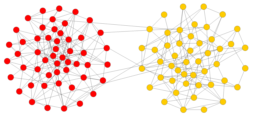
Figure 4.
In the last phase the network is entirely polarized in two homogeneous clusters. If the simulation is long enough all the links between the two poles will disappear.
To confirm the stability of this topological evolution we performed several simulation using the noisy strategy update rule. Even in this situation the network will attain a polarized state but due to the stochastic strategy fluctuations the two main clusters almost never reach a completely disconnected state and the modularity remains slightly lower () compared to the noiseless case.
As a second kind of numerical experiment, we asked how the population would react when, in a polarized social situation, a few connected players of one of the clusters suddenly switch to the opposite strategy. The results of a particular but typical simulation are shown in Figure 5. Starting from the clusters obtained as a result of the co-evolution of strategies and network leading to Figure 4, a number of “red” individuals replace some “yellow” ones in the corresponding cluster. The evolution is very
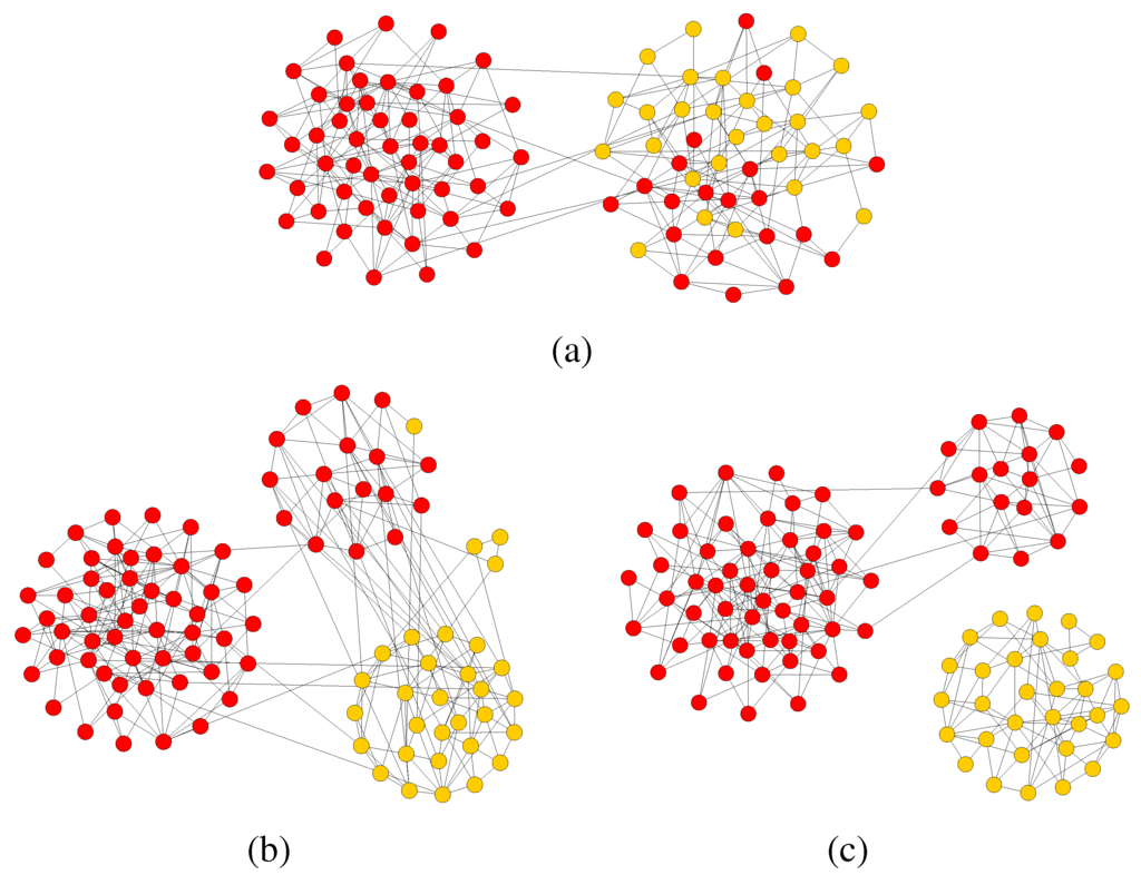 interesting: after some time the two-cluster structure disappears and is replaced by a different network in which several clusters with a majority of one or the other strategies coexist. However, these intermediate structures are unstable and, at steady state one recovers essentially a situation close to the initial one, in which the two poles form again but with small differences with respect to the original one. Clearly the size of the clusters is different from that of before the invasion. Even in this case, if the evolution time is long enough, the two components can become disconnected at the end. This means that, once formed, polar structures are rather stable, except for noise and stochastic errors. Moreover, we observed that at the beginning the invasion process the modularity drops slightly due to the strong reorganization of the network but then it increases again and often reaches a higher value with respect to the previous state. In the case shown here, the final modularity is . The same happens in the larger networks where, after the invasion process Q reaches values of .
Figure 5.
(a) A consistent amount of mutant is inserted in one of the two clusters. (b) This invasion perturbs the structure of the population that starts to reorganize. (c) With enough evolution time the topology reaches a new polarized quasi-equilibrium.
5. Results for General Coordination Games
In this section we show the numerical results for the Stag Hunt class of coordination games. We recall that, unlike pure coordination games, in Stag Hunt games there is risk in coordinating on the Pareto-efficient strategy and thus agents may wish to reduce their aspirations by playing the socially inferior strategy for fear of being “betrayed” (see Section 2.1).
The simulation parameters are the same as for coordination games, see Section 4.1, except that now the game parameter space is more complex. For the Stag Hunt the ordering of payoffs is , and we have studied the portion of the parameters’ space defined by and , , and , as is customarily done [10]. The plane has been sampled with a grid step of .
In order to find out whether a change in the strategy update dynamics would make a difference in the results, we have used, besides the already described best response dynamics, another update rule which is related to replicator dynamics [1,3]. Instead of considering a mixing population, the version of replicator dynamics used here is modified to take into account the local nature of interaction networks as proposed by [27]. It assumes that the probability of switching strategy is a monotonic increasing function ϕ of the payoff difference; here ϕ is a linear function. First, a player i is randomly chosen from the population to be updated with uniform probability and with replacement. To update its strategy another player j is next drawn uniformly at random from i’s neighborhood . Then, strategy is replaced by with probability:
in which
is the accumulated payoff collected by player i at time step t after having played with all his neighbors . The major difference with standard replicator dynamics is that two-person encounters between players are only possible among neighbors, instead of being drawn from the whole population.
5.1. Strategy Distribution at Steady State
The following Figure 6 and Figure 7 show the average fraction of strategy α (light color) and β (darker color) respectively at steady state for best response dynamics and replicator dynamics, and for three values of the rewiring frequency q increasing from left to right. Initially there is an equal amount of α and β players randomly distributed in the network nodes. The first thing to notice is that the trend is the same, i.e., higher frequencies of link rewiring favor the Pareto-efficient result for both dynamics, although this happens to a lesser extent for best response. The reason is that best response confirms the players in what they are doing: the best response to α is α and to β it is β but, on the whole, the possibility of link rewiring allows unsatisfied α-strategists to cut a link with a β-strategist and to search for another α in the next to first neighborhood. Since the data plotted in the figures are average values, it is also important to point out that, actually, in all runs the final steady state is constituted by a monomorphic population, i.e., only one strategy is present. This is coherent with standard results on Stag Hunt games which show that polymorphic populations are unstable and that the dynamics should converge to one of the pure states [3,18,19,20].
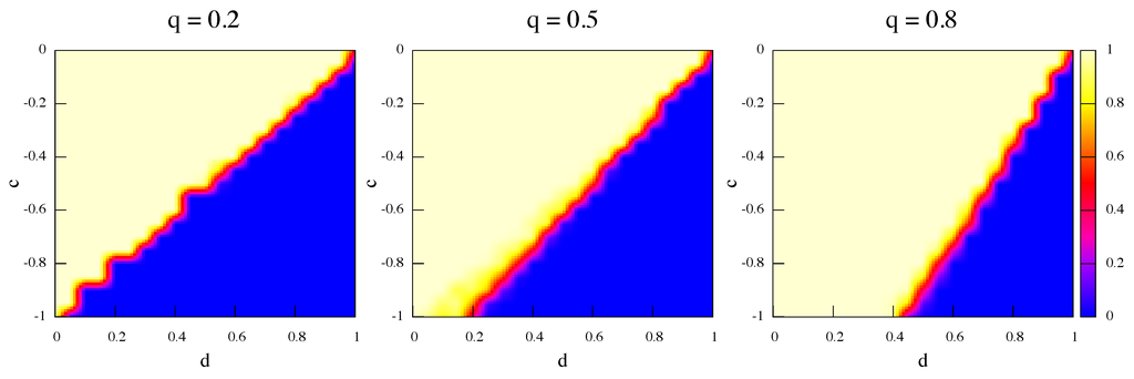
Figure 6.
Average strategy proportions over 50 independent runs in the game’s phase space at steady state. Initially α and β are equally represented. Update rule is best response and rewiring frequency q increases from left to right.
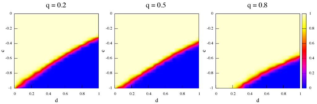
Figure 7.
Average strategy proportions over 50 independent runs in the game’s phase space at steady state. Initially α and β are equally represented. Update rule is replicator dynamics and rewiring frequency q increases from left to right.
The update rules used are both noiseless, in the sense that, apart from the implicit probabilities used in the dynamics, no exogenous noise simulating strategic errors or trembles has been added. When a small amount of error probability of is added in the best response case the results change very little and are not shown.
One might also ask what happens when initially the strategies are not present in equal amounts and, in particular, whether network and rewiring effects may help the socially efficient strategy α to proliferate when it starts in the minority. Figure 8 and Figure 9 are the same as Figure 6 and Figure 7 but this time strategy α is only of the total initially. It is apparent that, even when α-strategists are the minority, they can occupy a sizeable region of the phase space thanks to rewiring effects. Indeed, by increasing the rewiring frequency the size of the α region increases as well. The effects are present for both dynamics but they are more marked in the best response case (Figure 8). As a further probe, we have also simulated the evolution of populations with only α initially and the results, not shown here, are that the α strategy proliferates in a non-negligible region of the parameter space and the more so the higher the relinking frequency.
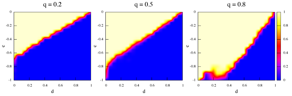
Figure 8.
Average strategy proportions over 50 independent runs in the game’s phase space at steady state. Initially α players are of the total. Update rule is best response and rewiring frequency q increases from left to right.
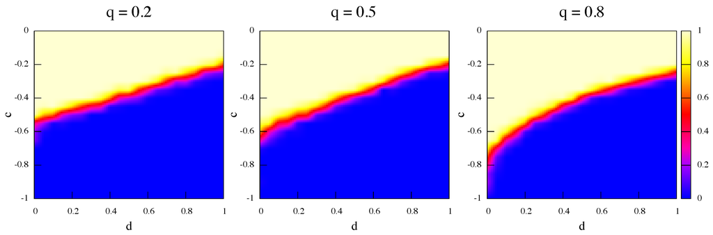
Figure 9.
Average strategy proportions over 50 independent runs in the game’s phase space at steady state. Initially α players are of the total. Update rule is replicator dynamics and rewiring frequency q increases from left to right.
5.2. Network Features
In this section we present a statistical analysis of some of the global and local properties of the networks that emerge when the pseudo-equilibrium states of the dynamics are attained. We do not strive for a complete analysis: this would take too much space; just a few topological features should be already useful to get a clearer picture. The graphs used for the analysis are the undirected, unweighted versions . An important global network statistics is the average clustering coefficient C. The clustering coefficient of a node i is defined as , where is the number of edges in the neighborhood of i and is i’s degree. Thus measures the amount of “cliquishness” of the neighborhood of node i and it characterizes the extent to which nodes adjacent to node i are connected to each other. The clustering coefficient of the graph is simply the average over all nodes: [5]. In Figure 10 we report for each grid point the average value of C over 50 realizations of . The figure shows that in general C increases with increasing q which is reasonable, as higher q values mean more rewiring and thus more transitive closure of triangles in the neighborhood. In particular, we have remarked that C is especially high in the proximity of the transition zone between β and α regions. We also note that the clustering of α-strategists networks are higher than those of β-strategists. Indeed, in the relinking process, links tends to be stable as both players get the maximum payoff. On the other hand, links will be unstable since the α end will try to dismiss the link, while the β end tries to keep it. As for the links, they also tend to be unstable for both agents will in the average try to chase for an α. When αs become rearer in the population the links are more difficult to stabilize and local structure does not emerge.
To give a qualitative idea of the network self-organization, we compare C values in the α and β regions with the values expected for the initial random graph. Random graphs are locally homogeneous and for them C is simply equal to the probability of having an edge between any pair of nodes independently. In contrast, real networks have local structures and thus higher values of C. For example, with , C can be as high as in the α region close to the transition, and as low as in the β region. It is thus apparent that the networks self-organize and acquire local structure for α networks as C is much higher than that of the random graph with the same number of nodes and edges, which is . In the β region there is barely more clustering than for a random graph. Given that the model favors rewiring a link toward a neighbor’s neighbor, it is obvious that the clustering coefficient will tend to increase and thus the effect was expected. Nevertheless, this transitive closure is a well known social phenomenon and the model successfully simulates it.
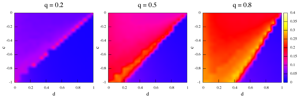
Figure 10.
Average clustering coefficients of steady-state networks; relinking frequency q increases from left to right. Equal initial proportions of α and β strategies and strategy update is by best response.
Another important quantity is the degree distribution function. The degree distribution function of a graph represents the probability that a randomly chosen node has degree k [5]. Random graphs are characterized by distributions of Poisson form , while social and technological real networks often show long tails to the right, i.e., there are nodes that have an unusually large number of neighbors [5]. In some extreme cases the distribution has a power-law form ; the tail is particularly extended and there is no characteristic degree.
In our simulations the population graph always starts random, i.e., has a Poisson degree distribution. It would be interesting to see whether the graphs remain random after the co-evolutionary process stabilizes in a steady state, or whether they acquire some more structure. Figure 11 shows the degree distribution functions sampled at two points in the plane. One point is in the α-stable region and the other is in the β-stable one. The third dotted curve is shown for comparison and corresponds to the initial random graph which has a Poisson with . Both curves at steady state deviate from the random graph distribution but, while the degree distribution of the network of β players is still rather close to Poisson, the α network (thick curve) shows a distribution that has a longer tail to the right, i.e., there is a non-negligible quantity of nodes that have more connections. Together with the increase of the clustering coefficient seen above, this shows that α networks have acquired more structure than β networks during the co-evolutionary process. It appears that α strategists use the relinking possibility in such a way that more α clusters are created, thus protecting them from β “exploiters”. The curves shown are for ; for lower values of q the effect is the same but less marked as .

Figure 11.
Average empirical degree distribution functions for the initial random graphs (dotted line), steady-state graphs in the α-dominant region of the parameters’ space (thick curve), and in the β-dominant region (dashed line) All distributions are discrete, continuous curves are just a guide for the eye.
6. Conclusions
In this paper we propose and simulate numerically a model in which a population of agents interacting according to a network of contacts play games of coordination with each other. The agents can update their game strategy according to their payoff and the payoff of their neighbors by using simple rules such as best response and replicator dynamics. In addition, the links between agents have a strength that changes dynamically and independently as a function of the relative satisfaction of the two end points when playing with their immediate neighbors in the network. A player may wish to break and redirect a tie to a neighbor if it is unsatisfied. As a result, there is co-evolution of strategies in the population and also of the graph that represents the network of contacts.
We have applied the above model to the class of coordination games, which are important paradigms for collaboration and social efficiency. For pure coordination games, the networks co-evolve towards the polarization and, in some cases, even the splitting of the graph into two distinct connected components of different strategies. Even with a relatively small rewiring frequency polarization is reached relatively quickly. This metaphorically represents the segregation of norm-following subpopulations in larger populations. In the case of general coordination games the issue is whether the socially efficient strategy, i.e., the Pareto-dominant one, may establish in the population. While results in well-mixed and static networked populations tend to favor the risk-dominant, and thus socially inefficient outcome, our simulation results show that the possibility of refusing neighbors and choosing different partners increases the success rate of the Pareto-dominant equilibrium. Although the model is extremely simplified, the possibility of link redirection is a real one in society and thus these results mean that some plasticity in the network contacts may have positive global social effects.
Acknowledgements
We gratefully acknowledge financial support by the Swiss National Science Foundation under contract 200020-119719.
References
- Vega-Redondo, F. Economics and the Theory of Games; Cambridge University Press: Cambridge, UK, 2003. [Google Scholar]
- Nowak, M.A. Five rules for the evolution of cooperation. Science 2006, 314, 1560–1563. [Google Scholar] [CrossRef] [PubMed]
- Gintis, H. Game Theory Evolving; Princeton University Press: Princeton, NJ, USA, 2009. [Google Scholar]
- Nowak, M.A.; May, R.M. Evolutionary games and spatial chaos. Nature 1992, 359, 826–829. [Google Scholar] [CrossRef]
- Newman, M.E.J. The structure and function of complex networks. SIAM Rev. 2003, 45, 167–256. [Google Scholar] [CrossRef]
- Szabó, G.; Fáth, G. Evolutionary games on graphs. Phys. Rep. 2007, 446, 97–216. [Google Scholar] [CrossRef]
- Santos, F.C.; Pacheco, J.M. Scale-Free Networks provide a unifying framework for the emergence of cooperation. Phys. Rev. Lett. 2005, 95, 098104. [Google Scholar] [CrossRef] [PubMed]
- Luthi, L.; Pestelacci, E.; Tomassini, M. Cooperation and community structure in social networks. Physica A 2008, 387, 955–966. [Google Scholar] [CrossRef]
- Skyrms, B. The Stag Hunt and the Evolution of Social Structure; Cambridge University Press: Cambridge, UK, 2004. [Google Scholar]
- Roca, C.P.; Cuesta, J.A.; Sánchez, A. Evolutionary Game theory: temporal and spatial effects beyond replicator dynamics. Phys. Life Rev. 2009, 6, 208–249. [Google Scholar] [CrossRef] [PubMed]
- Luthi, L.; Giacobini, M.; Tomassini, M. A minimal information prisoner’s dilemma on evolving networks. In Artificial Life X; Rocha, L.M., Ed.; The MIT Press: Cambridge, MA, USA, 2006; pp. 438–444. [Google Scholar]
- Santos, F.C.; Pacheco, J.M.; Lenaerts, T. Cooperation prevails when individuals adjust their social ties. PLOS Comp. Biol. 2006, 2, 1284–1291. [Google Scholar] [CrossRef] [PubMed]
- Zimmermann, M.G.; Eguíluz, V.M. Cooperation, social networks, and the emergence of leadership in a prisoner’s dilemma with adaptive local interactions. Phys. Rev. E 2005, 72, 056118. [Google Scholar] [CrossRef] [PubMed]
- Perc, M.; Szolnoki, A. Coevolutionary Games—A mini review. Biosystems 2010, 99, 109–125. [Google Scholar] [CrossRef] [PubMed]
- Pestelacci, E.; Tomassini, M.; Luthi, L. Evolution of cooperation and coordination in a dynamically networked society. J. Biol. Theory 2008, 3, 139–153. [Google Scholar] [CrossRef]
- Tomassini, M.; Pestelacci, E.; Luthi, L. Mutual trust and cooperation in the evolutionary Hawks-Doves Game. Biosystems 2010, 99, 50–59. [Google Scholar] [CrossRef] [PubMed]
- Jackson, M.O. Social and Economic Networks; Princeton University Press: Princeton, NJ, USA, 2008. [Google Scholar]
- Kandori, M.; Mailath, G.; Rob, R. Learning, mutation, and long-run equilibria in games. Econometrica 1993, 61, 29–56. [Google Scholar] [CrossRef]
- Ellison, G. Learning, local interaction, and coordination. Econometrica 1993, 61, 1047–1071. [Google Scholar] [CrossRef]
- Robson, A.J.; Vega-Redondo, F. Efficient equilibrium selection in evolutionary games with random matching. J. Econ. Theory 1996, 70, 65–92. [Google Scholar] [CrossRef]
- Morris, S. Contagion. Rev. Econ. Stud. 2000, 67, 57–78. [Google Scholar] [CrossRef]
- Skyrms, B.; Pemantle, R. A dynamic model for social network formation. Proc. Natl. Acad. Sci. USA 2000, 97, 9340–9346. [Google Scholar] [CrossRef] [PubMed]
- Schelling, T. The Strategy of Conflict; Harvard University Press: Cambridge, MA, USA, 1960. [Google Scholar]
- Fortunato, S. Community detection in graphs. Phys. Rep. 2010, 486, 75–174. [Google Scholar] [CrossRef]
- Newman, M.E.J.; Girvan, M. Finding and evaluating community structure in networks. Phys. Rev. E 2004, 69, 026113. [Google Scholar] [CrossRef] [PubMed]
- Newman, M.E.J. Modularity and community structure in networks. Proc. Natl. Acad. Sci. USA 2006, 103, 8577–8582. [Google Scholar] [CrossRef] [PubMed]
- Hauert, C.; Doebeli, M. Spatial structure often inhibits the evolution of cooperation in the snowdrift game. Nature 2004, 428, 643–646. [Google Scholar] [CrossRef] [PubMed]
- 1The active agent is chosen with uniform probability and with replacement.
- 2With the above simulated process one cannot properly speak of true equilibrium states in the strict mathematical sense.
© 2010 by the authors; licensee MDPI, Basel, Switzerland. This article is an Open Access article distributed under the terms and conditions of the Creative Commons Attribution license http://creativecommons.org/licenses/by/3.0/.