The ‘Hawk-Dove’ Game and the Speed of the Evolutionary Process in Small Heterogeneous Populations

Abstract

I study the speed of the evolutionary process on small heterogeneous graphs using the Hawk-Dove game. The graphs are based on empirical observation data of grooming interactions in 81 primate groups. Analytic results for the star graph have revealed that irregular graphs can slow down the evolutionary process by increasing the mean time to absorption. Here I show that the same effects can be found for graphs representing natural animal populations which are much less heterogeneous than star graphs. Degree variance has proven to be a good predictor for the mean time to absorption also for these graphs.

1. Introduction

Game theory was originally brought up by John von Neumann and Oskar Morgenstern [1] to study economic behaviour and decision making in humans. In the 1970s game theory was adopted by biologists to make predictions about evolutionary processes [2,3,4,5]. In evolutionary game theory the payoff from a game is linked with the fitness (i.e., the reproductive success) of an individual. Strategies are coded by genes. Individuals who receive higher payoffs reproduce at higher rates and, consequently, their genes spread in the population. As a result advantageous strategies become more abundant. Evolutionary game theory differs in several important aspects from classical game theoretic analyses. To begin with, choice of strategies is handed over to natural selection, which means that it does not require assumptions about rationality or cognitive abilities of the agents. Furthermore, rather than studying the outcome of a game in a two-player setting, evolutionary game theory focuses on the frequencies of different strategies in larger populations. And finally, as a consequence of the previous point, evolutionary game theory deals usually with dynamic systems. More recently, evolutionary game theory has been taken up by social scientists where the evolutionary dynamics are interpreted in terms of cultural evolution [for reviews see: 6,7]. In this context reproduction is interpreted as social learning. That is, successful strategies are imitated by other individuals and, hence, a strategy can spread in a population through social adoption.

Originally, models of evolutionary games were developed for large populations where strategy frequencies could be approximated by differential equations [8]. However, as real populations are not infinitely large, interest has turned to evolutionary games in finite populations [9,10,11]. Modelling evolutionary processes for finite populations brings along some fundamental changes. The evolutionary dynamics are no longer described by deterministic differential equations, but they require a stochastic formulation. The abundance of individuals following a specific strategy is given in absolute numbers rather by continuous proportions. And, as the population is finite, it is possible –and in most cases inevitable- that the population will end up in a state where all individuals are of the same type (pursue the same strategy) within finite time. If a population has reached such a state, and if spontaneous mutations of novel strategies are not considered, the population will stay in that state forever. The population is in an absorbing state and the strategy has reached fixation [12]. The absorption time is the average time that it takes a population with a given initial condition to reach one of the absorbing states. From the perspective of a specific strategy one can distinguish between the two absorbing states, which are extinction (no individual of the respective strategy left) and fixation (the whole population consists of individuals of that strategy).

The probability that a specific strategy will reach fixation depends on the inheritance and selection process, the relative fitness of the strategy (in relation to the fitness of the other strategies) and its initial abundance [10]. Several inheritance processes have been studied extensively, each trying to mimic different aspects of natural populations [13]. In this paper I will focus on the Moran process [14,15]. In this process one individual is chosen at random for reproduction, though with a probability proportional to its fitness. This individual produces one offspring which replaces a randomly chosen individual. This process ensures that the population size stays constant. It is meant to mimic the case where a population of individuals has reached the carrying capacity for its habitat and, hence, cannot increase any more. If all individuals have the same fitness, then the probability that one specific individual reaches fixation is given by P = 1/N, where N is the size of the population. In a population where all individuals are of one type with fitness 1, a single mutant with a fitness value of $r\ne 1$ has a fixation probability of

$$P_{Moran}=\frac{1-(1/r)}{1-{(1/r)}^N}.$$

(1)

As in the Moran process the offspring of the reproducing individual is replacing a randomly chosen individual, any individual is equally likely to be affected by the reproduction process of any other individual. In evolutionary biology a population that fulfils this property is referred to as well-mixed or panmictic population [16]. However, real populations are rarely well-mixed. Many populations have a certain spatial structure –that is, individuals directly affect only other individuals in their vicinity and neighbouring individuals will usually share part of their neighbourhood. Early attempts to incorporate population structure in evolutionary games focused on spatial structure by studying the evolution of interactive strategies on regular lattices [e.g. 17,18,19,20,22,23]. Evolutionary games on lattices lead to some interesting dynamics that could not be observed in well mixed populations. More recently this approach was generalized by replacing regular lattices by graphs which allow to model any possible population structure [24,25,26,27,28,29,30,31,32,33].

Fixation probabilities of various strategies have been studied extensively on many different population structures, however, the time to fixation –or, more generally- the time needed to reach an absorbing state received only little attention, so far. This is very unfortunate, as fixation and absorption time are very important for the understanding of two aspects of evolutionary processes. Firstly, given a certain population size and a certain fitness advantage of a mutant strategy type, is it possible that this strategy reaches fixation within a realistic time frame? While for some evolutionary scenarios analytic models showed that a certain strategy should reach fixation with a very high probability, some behavioural ecologists were concerned that the number of generations needed to reach such a state could ‘easily exceed the age of the universe’ [34]. Thus, investigating fixation times for realistic population sizes and structures addresses the applicability of such abstract evolutionary models for explaining organismic evolution. And secondly, absorption times can help to predict the phenotypic variability one should expect in a specific population. If one assumes, that mutant strategies enter the population at an approximately constant low rate, then the number of different phenotypes present in a population at any time will depend on how fast strategies would reach fixation or get extinct [12,25].

A derivation of the mean absorption time for well-mixed, infinite populations was first delivered by Karlin and Taylor [35] and for finite populations by Antal and Scheuring [36]. Broom and colleagues [37] took an analytical approach to derive the exact solutions of the stochastic evolutionary dynamics of the Hawk-Dove game for complete graphs, rings, and the star graph. It was argued that the Hawk-Dove game is particularly interesting because in infinite well-mixed populations the evolutionary dynamics yield a mixture of both strategies, and consequently fixation in the finite population case should be very slow [36,37]. As in all previous studies graph structures were highly arbitrary, it is difficult to predict how the structure of real-world populations should affect absorption times. In this study I, therefore, investigated the absorption times of a Hawk-Dove game on graphs that represent real-world group structures of primates.

2. Data Collection

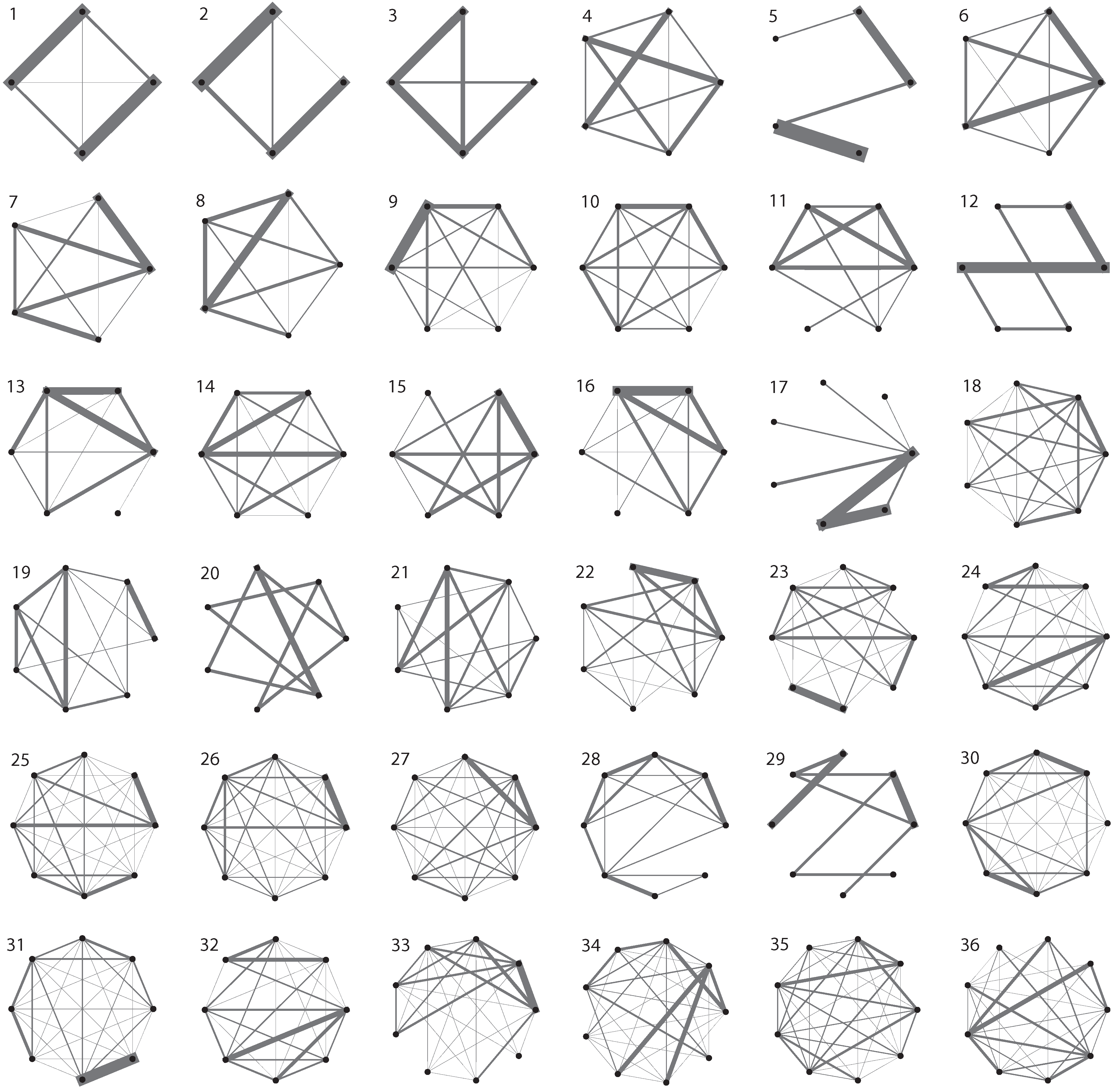
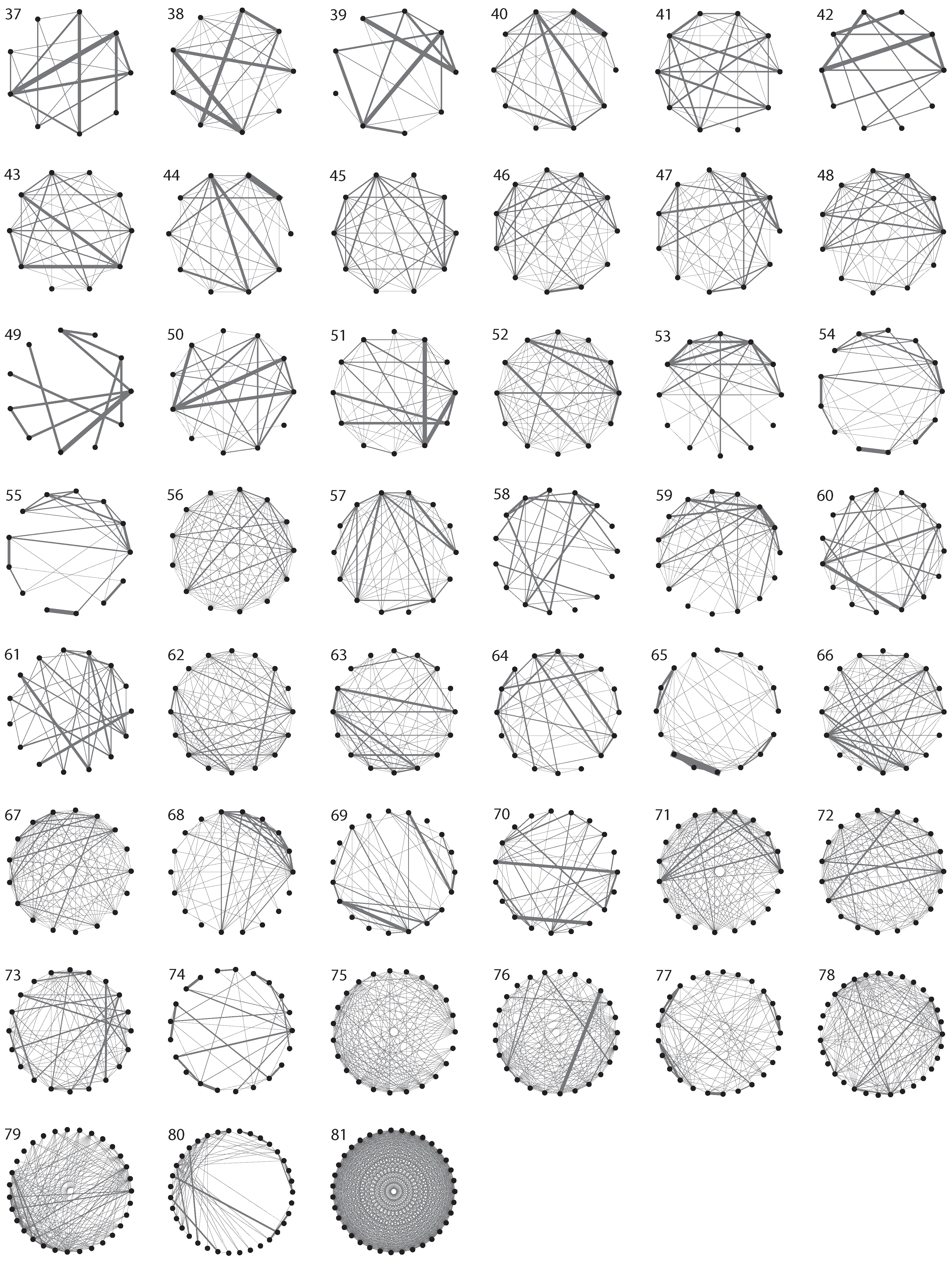
The used dataset consists of the grooming interaction matrices (Figure 1) of 81 primate groups [38]. The data were partly taken from the literature and partly from unpublished material either collected by the authors or shared by colleagues. The dataset comprises 35 species and 16 genera. Grooming is the search for and removal of ecto-parasites from the fur of the interaction partner. Besides its hygienic function it serves as an important social behaviour that the animals use to establish social relationships [39].

Figure 1. Graphs based on primate grooming networks. Edges denote grooming interactions between individuals; edge weights indicate interaction frequencies. Grooming networks from: Macaca arctoides (68,6,7,72,37), fuscata (54,17,46,47,74,55,57,31,73,65), fascicularis (24,40,70,32,44), radiata (62,75), mulatta (63), tonkeana (76), assamensis (71), sylvanus (52,22,61), Cercopithecus neglectus (9), campbelli (59), mitis (64,67), Chlorocebus aethiops (26,18,27,78,19,21,45), Cercocebus torquatus (81), Miopithecus talapoin (25), Erythrocebus patas (69,30), Trachypithecus pileatus (53), Presbytis entellus (56,42), Colobus guereza (8), Papio anubis (80), papio (34,77,79), cynocephalus (28), Theropithecus gelada (12), Mandrillus sphinx (5), Piliocolobus tephrosceles (66), Pan troglodytes (58,23,41,35,48,43,36), paniscus (42), Cebus apella (51,15,16,50), capucinus (10), olivaceus (33), Callithrix jacchus (3,11,29), Alouatta caraya (4), fusca. (13), palliata (49,20), Ateles geoffroyi (60,38,39), Eulemur macaco (1,2).

Figure 1. Graphs based on primate grooming networks. Edges denote grooming interactions between individuals; edge weights indicate interaction frequencies. Grooming networks from: Macaca arctoides (68,6,7,72,37), fuscata (54,17,46,47,74,55,57,31,73,65), fascicularis (24,40,70,32,44), radiata (62,75), mulatta (63), tonkeana (76), assamensis (71), sylvanus (52,22,61), Cercopithecus neglectus (9), campbelli (59), mitis (64,67), Chlorocebus aethiops (26,18,27,78,19,21,45), Cercocebus torquatus (81), Miopithecus talapoin (25), Erythrocebus patas (69,30), Trachypithecus pileatus (53), Presbytis entellus (56,42), Colobus guereza (8), Papio anubis (80), papio (34,77,79), cynocephalus (28), Theropithecus gelada (12), Mandrillus sphinx (5), Piliocolobus tephrosceles (66), Pan troglodytes (58,23,41,35,48,43,36), paniscus (42), Cebus apella (51,15,16,50), capucinus (10), olivaceus (33), Callithrix jacchus (3,11,29), Alouatta caraya (4), fusca. (13), palliata (49,20), Ateles geoffroyi (60,38,39), Eulemur macaco (1,2).

As grooming implies close proximity of the involved individuals, it indicates high levels of social tolerance and it has been shown to be a good predictors for overall spatial proximity [40,41]. While grooming episodes can be observed between most members of a primate community, the frequency how often two specific individuals are engaged in such an interaction varies drastically. To incorporate this important information about the quality of dyadic relationships it was suggested to represent the grooming network as a weighted graph, where edge weights are proportional to grooming frequencies [42].

3. Evolutionary Dynamics

The Hawk-Dove game was originally suggested by John Maynard Smith and George Price [4]. The basic idea of the Hawk-Dove game is that two individuals compete for a resource. The resource brings a benefit B to the one who wins it. Individuals can play one of two strategies: ‘Hawk’, meaning that they will fight for the resource, and ‘Dove’, which means that they will abandon the resource as soon as a conflict escalates into a fight. Fighting is, however, dangerous and the looser of a fight has to bear a cost C. If a Hawk meets a Hawk, they will fight and one of them will win the resource. Thus, the average payoff of a Hawk meeting a Hawk is (B-C)/2. If a Hawk meets a Dove the Dove immediately withdraws, so its payoff is zero, while the payoff of the Hawk is B. If two Doves meet, the one who first gets hold of the resource keeps it while the other does not fight for it. Thus, the average payoff for a Dove meeting a Dove is B/2. The strategic form of the game is given by the payoff matrix

$$Payof{f}_{Hawk,Dove}=\left(\begin{array}{cc}(B-C)/2& B\\ 0& B/2\end{array}\right).$$

(2)

I used Monte Carlo Markov Chain (MCMC) simulations to study the evolutionary dynamics on the graphs derived from the primate interaction data set. At the beginning a randomly chosen vertex of a monomorphic population of residents is replaced by a mutant which plays the opposing strategy. In every consecutive round the population is updated according to the following rules:

(1)

Each vertex plays with every of its neighbours one round of a Hawk-Dove game with the payoff matrix of equ. 2.

(2)

The fitness of a vertex is calculated as the sum of its payoffs from these games plus a background fitness value.

(3)

A vertex is chosen for reproduction with a probability proportional to its fitness.

(4)

A neighbour of the reproducing vertex is chosen with a probability proportional to the edge weight and replaced by a clone of the reproducing vertex.

This updating process is repeated until the population has reached one of the two absorbing states: either all vertices are of the residents’ strategy type or of the mutant’s type. The number of rounds it takes to reach the absorbing state is the absorption time.

The simulation of such an evolutionary process was repeated 10,000 times for each of the 81 different graphs representing the social systems of the primate groups and for each of the following seven conditions: (1-3) the fixed fitness scenario with residents having fitness 1, mutants having fitness r, with r = 0.5, 1, and 1.5 respectively, (4-5) a population of Doves and a single Hawk mutant with C = 2 and 13 respectively, and (6-7) a population of Hawks with a single Dove mutant with, again, C = 2 and 13. The mean absorption times for the graphs were compared with the baseline absorption time for the homogeneous complete graph with edge weights of unity (representing a well-mixed group). Baseline absorption times t_abs were calculated following Traulsen and Hauert [43] as

$$t_{abs}=\frac{1}{1+{\displaystyle {\sum }_{k=1}^{N-1}{\displaystyle {\prod }_{j=1}^k{\gamma }_j}}}{\displaystyle {\sum }_{k=1}^{N-1}{\displaystyle {\sum }_{l=1}^k\frac{1}{T_l^{+}}}}{\displaystyle \prod _{j=l+1}^k{\gamma }_j},$$

(3)

with ${\gamma }_j=T_j^{-}/T_j^{+}$, where $T_j^{+}$ is the probability to increase the number of mutants from j to j+1 and $T_j^{-}$ is the probability to decrease the number of mutants from j to j-1, with

$$T_j^{+}=\frac{j\times f(j)}{j\times f(j)+(N-j)\times g(j)}\frac{N-j}{N},$$

(4)

$$T_j^{-}=\frac{(N-j)\times g(j)}{j\times f(j)+(N-j)\times g(j)}\frac{j}{N},$$

(5)

$$f(j)=\frac{(j-1)(B-C)/2+(N-j)B}{N-1}$$

(6)

and

$$g(j)=\frac{(N-j-1)B/2}{N-1}.$$

(7)

4. Results

4.1. Fixed Fitness Case

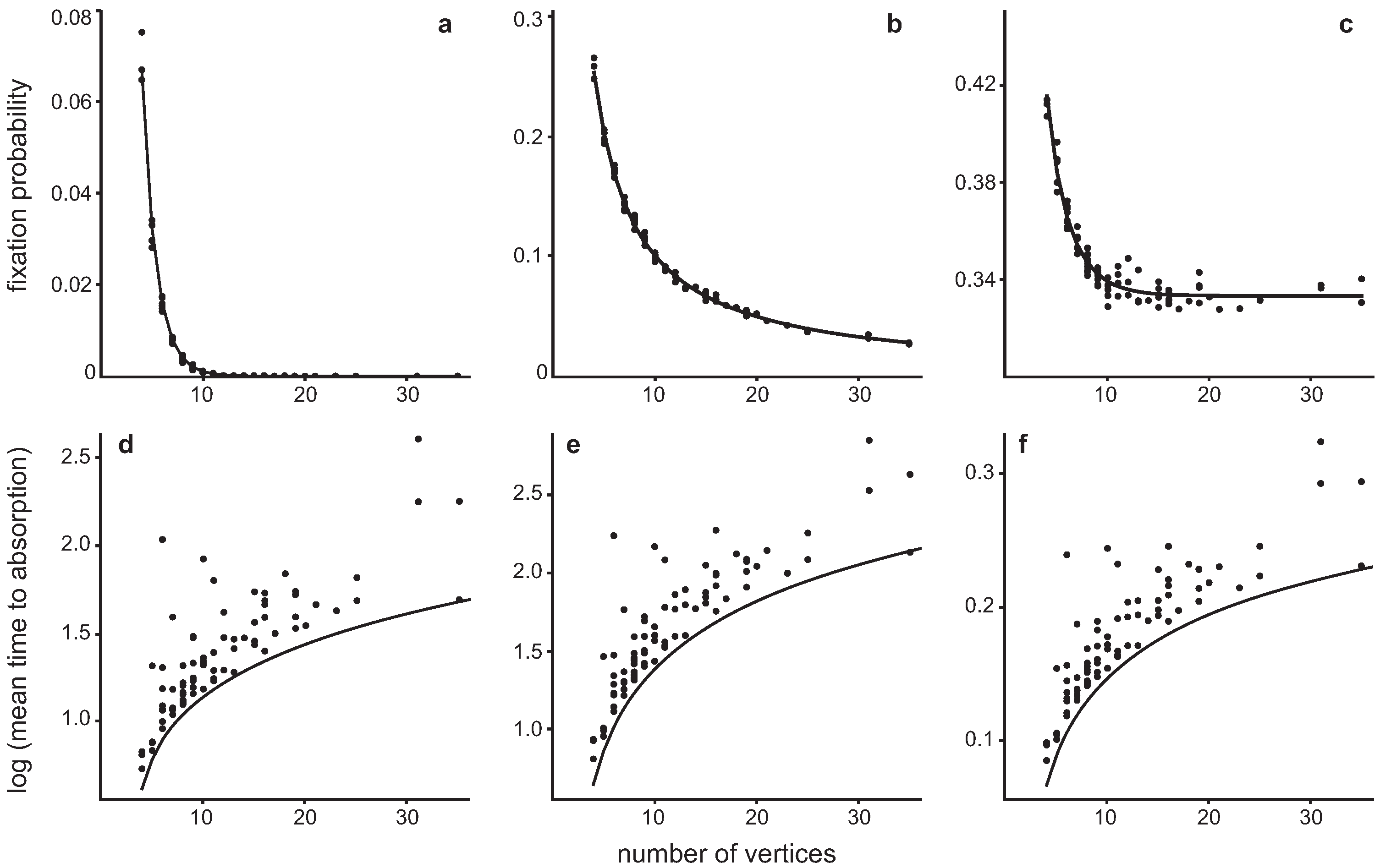
Before studying the Hawk-Dove game I investigated the simpler case where the fitness is independent of the identity of the interaction partner, residents have fitness 1 and mutants have fitness r. I simulated the evolutionary dynamics for r = 0.5, 1, and 1.5. The first case resembles a disadvantageous mutation where the fitness of the mutant is smaller than that of the residents, the second case represents a fitness-neutral mutation, and in the third case the mutation is advantageous. The expected fixation probability for a single mutant in a well-mixed population is given by equ. 1. Fixation probabilities for the 81 primate graphs are given in Figure 2a-c (see also electronic supplementary information). Overall, the fixation probabilities were quite close to the expected value for well mixed populations (GLM, identity link, N = 81, r = 0.5: R² = 0.99; r = 1.0: R² = 99; r = 1.5: R² = 0.94), though variation was slightly higher in the case of advantageous mutations (Figure 2c). Expected times to absorption for the complete graphs representing well mixed populations were calculated using equ. 3. The mean time to absorption was overall higher for the primate graphs than the expected absorption times for the complete graphs of equal size (Figure 2d-f).

Figure 2. Fixation probabilities and mean times to absorption for the fixed fitness case. The resident strategy has a fitness of 1 and the mutant has a fitness of r with (a, d) r = 0.5, (b, e) r = 1.0, (c, f) r = 1.5. Dots give mean values for 10,000 simulations for each of the 81 primate graphs and the solid line gives the expected value for a well mixed population.

Figure 2. Fixation probabilities and mean times to absorption for the fixed fitness case. The resident strategy has a fitness of 1 and the mutant has a fitness of r with (a, d) r = 0.5, (b, e) r = 1.0, (c, f) r = 1.5. Dots give mean values for 10,000 simulations for each of the 81 primate graphs and the solid line gives the expected value for a well mixed population.

4.2. Invasion of a single Hawk in a population of Doves

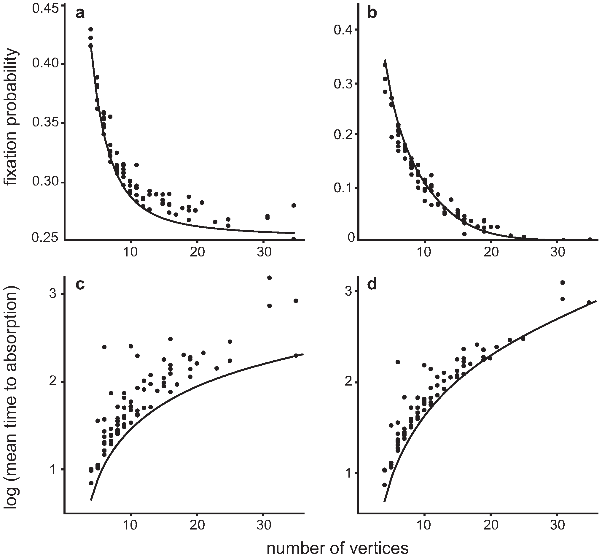
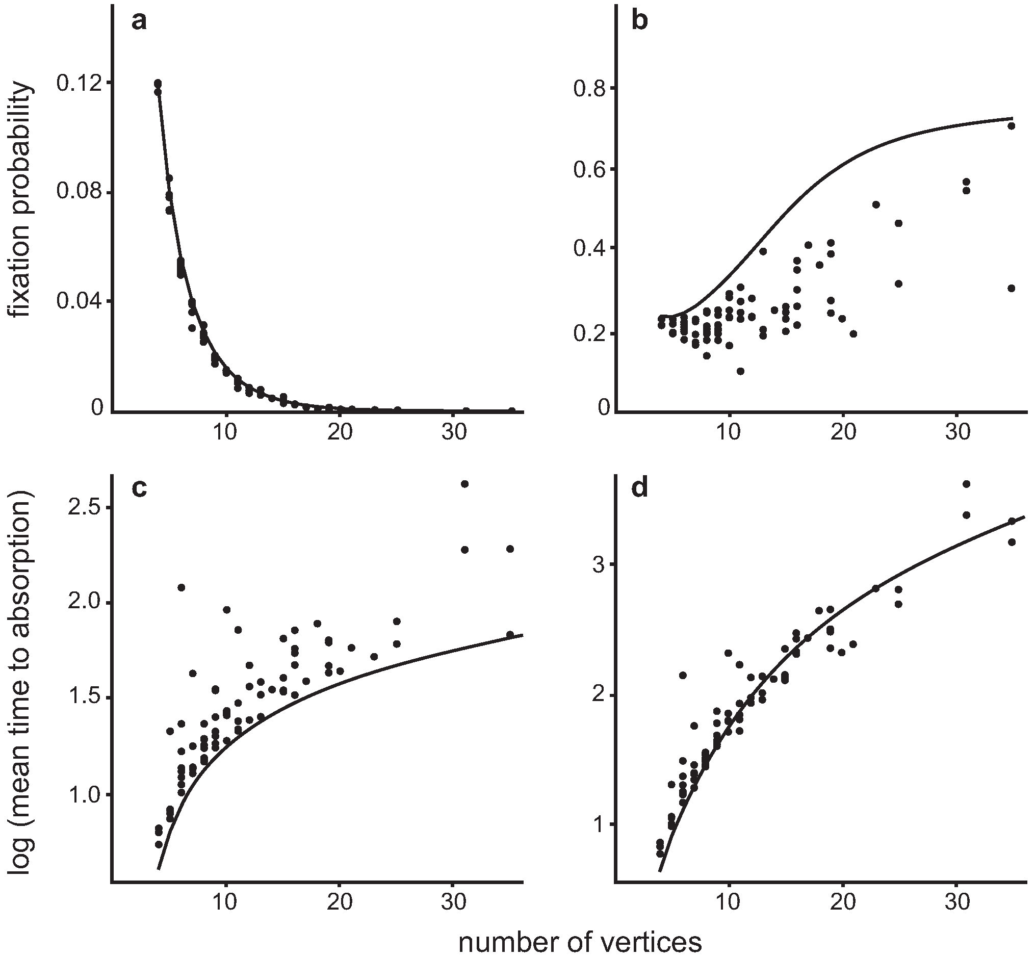
Invasion dynamics of a single mutant Hawk in a population of Doves was studied for two scenarios which differed in the cost C associated with loosing a fight. In accordance with Broom et al. [37] I have chosen C = 2 and 13, while B = 5 in both cases and the games are played in populations with a background fitness of F_B = 5. The first scenario resembles, therefore, the case where the fighting costs are smaller than the benefits B, while in the second scenario the fighting costs exceed the benefits. For C = 2 (smaller fighting costs) fixation of a mutant Hawk in a population of Doves was overall higher (in 76 out of 81 cases) in the structured primate graphs than the expectation for well-mixed populations (Figure 3a). The mean time to absorption, too, was clearly higher for the primate graphs than the expectation for well mixed populations (Figure 3c). For C = 13 (higher fighting costs) the fixation rates for the primate graphs were closely scattered around the expected value for well mixed populations (GLM, identity link, R² = 0.97), being lower than the expected value in 32 cases and larger in 49 cases (Figure 3b). Mean times to absorption were –with two exceptions- higher for the structured primate graphs (Figure 3d).

Finally, I simulated the invasion of a single mutant Dove in a population of Hawks. The same parameter combinations were used as above. For C = 2 fixation rates on the primate graphs were more often slightly lower than the expectation for well mixed populations (69 of 81 cases), though, the deviation from the expected value was usually very small (R² = 0.99, Figure 4a). Absorption times for the primate graphs were, however, again higher than the expected values for well mixed populations (Figure 4c).

Figure 3. Fixation probabilities and mean times to absorption for a single Hawk invader. The Hawk-Dove game is played with a background fitness of F_B = 5 and a value of the resource of B = 5. Costs for loosing a fight are (a, c) C = 2 and (b, d) C = 13. Dots give mean values for 10,000 simulations for each of the 81 primate graphs and the solid line gives the expected value for a well mixed population.

Figure 3. Fixation probabilities and mean times to absorption for a single Hawk invader. The Hawk-Dove game is played with a background fitness of F_B = 5 and a value of the resource of B = 5. Costs for loosing a fight are (a, c) C = 2 and (b, d) C = 13. Dots give mean values for 10,000 simulations for each of the 81 primate graphs and the solid line gives the expected value for a well mixed population.

Figure 4. Fixation probabilities and mean times to absorption for a single Dove invader. The Hawk-Dove game is played with a background fitness of F_B = 5 and a value of the resource of B = 5. Costs for loosing a fight are (a, c) C = 2 and (b, d) C = 13. Dots give mean values for 10,000 simulations for each of the 81 primate graphs and the solid line gives the expected value for a well mixed population.

Figure 4. Fixation probabilities and mean times to absorption for a single Dove invader. The Hawk-Dove game is played with a background fitness of F_B = 5 and a value of the resource of B = 5. Costs for loosing a fight are (a, c) C = 2 and (b, d) C = 13. Dots give mean values for 10,000 simulations for each of the 81 primate graphs and the solid line gives the expected value for a well mixed population.

4.3. Invasion of a single Dove in a population of Hawks

For C = 13 the expected patterns change. The fixation probability of a single Dove in a population of Hawks follows an increasing sigmoid function. The fixation probabilities for the primate graphs, too, increased with group size, though they stayed clearly below the expected values for well mixed populations (Figure 4b). Due to this lower fixation probabilities for Doves the absorption times for the primate graphs were much closer to the expected value than they were in the case of low fighting costs. In 29 (out of 81) cases they are even lower than the expected values for complete graphs (Figure 4d).

4.4. Vertex degree and strength variance

Broom and colleagues [44] studied evolutionary dynamics on small-order graphs (with up to eight vertices) and found that the variation in the vertex degree can be used as an indicator for the fixation probability of a randomly placed mutant. We argued elsewhere [32,42] that quantitative differences in social interactions are an important characteristic of their social systems and, hence, we represented the primate interaction networks not as binary graphs but as weighted graphs –where edge weights represent interaction likelihoods. Consequently I took a slightly different approach to investigate to what extent the differences in absorption times can be explained by the graph’s heterogeneity. As one measures for heterogeneity I calculated the degree variance [45] given by

$$Va{r}_d=\frac{1}{N}{\displaystyle \sum _{i=1}^N{\left(k_i-\frac{\left|E\right|}{N}\right)}^2}$$

(8)

where k_i is the degree of vertex i and E is the edge set of the graph. Furthermore I calculated the strength variance accordingly as

$$Va{r}_s=\frac{1}{N}{{\displaystyle \sum _{i=1}^N\left(s_i-\frac{{\displaystyle {\sum }_{j=1}^N{s}_j}}{N}\right)}}^2,$$

(9)

where the vertex strength s is given by

$$s_i={\displaystyle {\sum }_{j=1}^N{w}_{ij}},$$

(10)

with w_ij being the weight of the edge connecting vertex i with vertex j.

After a Pearson product-moment correlation showed only a low collinearity between these two measures (N = 81, r = -0.21) I entered both variables as linear predictors for absorption time on the primate graphs into a general linear regression model for each of the seven simulations (Table 1). For both the fixed fitness scenarios and the Hawk invader scenarios this model could explain between 72 and 76 percent of the variance in the data. As the F-ratios suggested that the explanatory value of the model was mainly due to the degree variance I tested a reduced model with the degree variance as a single predictor variable. The explanatory value of this, simpler model was nearly as high as the one of the two-factor model (Table 1). Thus, despite clear heterogeneity in the edge weights, the mean time to absorption was only clearly affected by the vertex degree variance but not by the vertex strength variance.

Table 1. Degree and strength variance as predictors for absorption times. Results of general linear models (GLMs) with identity link function fitted to absorption times. Fixed: fixed fitness case, Hawk: a single Hawk invader, Dove: a single Dove invader. F-values and significance levels are given for a two-way ANOVA for the full model; ***: P < 0.001, ns: P > 0.05.

	Full model (vard+vars +vard vars) R2	F vard	P vard	F vars	P vars	Reduced model (vard) R2
Fixed r = 0.5	0.75	255.0	***	2.5	ns	0.73
Fixed r = 1.0	0.72	196.3	***	0.0	ns	0.72
Fixed r = 1.5	0.76	242.3	***	0.2	ns	0.76
Hawk C = 2	0.74	223.2	***	0.1	ns	0.74
Hawk C = 13	0.72	200.0	***	1.7	ns	0.71
Dove C = 2	0.75	227.1	***	1.5	ns	0.73
Dove C = 13	0.72	196.9	***	0.3	ns	0.72

Table 1. Degree and strength variance as predictors for absorption times. Results of general linear models (GLMs) with identity link function fitted to absorption times. Fixed: fixed fitness case, Hawk: a single Hawk invader, Dove: a single Dove invader. F-values and significance levels are given for a two-way ANOVA for the full model; ***: P < 0.001, ns: P > 0.05.

	Full model (vard+vars +vard vars) R2	F vard	P vard	F vars	P vars	Reduced model (vard) R2
Fixed r = 0.5	0.75	255.0	***	2.5	ns	0.73
Fixed r = 1.0	0.72	196.3	***	0.0	ns	0.72
Fixed r = 1.5	0.76	242.3	***	0.2	ns	0.76
Hawk C = 2	0.74	223.2	***	0.1	ns	0.74
Hawk C = 13	0.72	200.0	***	1.7	ns	0.71
Dove C = 2	0.75	227.1	***	1.5	ns	0.73
Dove C = 13	0.72	196.9	***	0.3	ns	0.72

5. Discussion

The mean time to absorption is an important variable that deserves more attention as it has received so far. Broom and colleagues [37] have shown that on certain artificial graphs absorption was delayed in comparison to complete graphs. Here I showed that the same effect can be found for graphs representing real-life animal populations (primate groups). This was the case for the fixed fitness scenarios, irrespectively of whether the mutation brought a fitness advantage or disadvantage and also for the case of a single Hawk invader in the Hawk-Dove game, irrespectively of the fighting costs. For the scenario of a single Dove invader and high fighting costs the outcome differed insofar as the reduced fixation likelihood for the Dove mutation resulted in absorption times that were overall quite close to –and sometimes even lower than- the expected times for well mixed populations.

The graphs’ heterogeneity could be ascribed to two sources of variation: variance in the degree of the vertices and variance in the edge weights, and consequently the vertex strength. However, in contrast to my original expectations, linear model fitting suggests that only the former clearly affects the mean absorption times of the graphs. Broom and colleagues [44] suggested that the vertex degree variance might act as a good predictor for mean absorption times. This study supports this claim by showing that this holds also for real-world networks that bring along additional ‘noise’ in terms of variance in the interaction likelihoods.

Besides the use of real-world network data and the inclusion of edge weights representing dyadic interaction likelihoods, the model of this study differs in one important aspect from the model applied by Broom et al. [44]: here the total payoff of a vertex is calculated as the sum of the payoffs from the dyadic games that it plays with all its neighbours, while Broom and colleagues calculated the average over the games with all neighbours. For well mixed populations both rules will yield the same results. However, as soon as the graphs are irregular, the outcome might differ quite markedly. Which rule is more adequate depends on the system one wants to model. Calculating the average can be interpreted in two ways. Firstly, one can think of a situation where a player that is connected with k neighbours competes with each neighbour for a resource that is only worth 1/k^th of the original value (and loosing a fight would also be less costly). This interpretation would, however, render the basic assumption of the original Hawk-Dove game –that the resource is not divisible. The second interpretation –which I would regard as more plausible- would be to assume that each vertex plays only a single game per round with a randomly chosen neighbour. The long term average over many such rounds would then equal the average from a single round played against all neighbours. The important consequence of averaging is, that each player competes for the same amount of resources –or, in terms of the ‘one-game-per-round’ interpretation, plays the same number of games. On the other hand, by summing up payoffs one assumes that the benefit (or the average benefit) of a resource is always the same, irrespectively of the number of neighbours that a vertex has and that the frequency with which a vertex competes with a specific neighbour is also independent of the number of neighbours. This means, however, that the vertices can vary in the number of games they play and in the amount of resources they can allocate.

In this study I aimed to include all aspects of heterogeneity that could be observed in the real world networks –which is, besides the topology, also the variation in the interaction likelihoods (represented by edge weights) and the likelihood with which a specific individual is seen as inter-actor (given by the vertex strength). As we can see, that in the primate networks some individuals engage in much more interactions than others, I did not want to exclude this source of variation by averaging, but I opted for summing up the payoffs of the games. That is, vertices with high vertex strength play more games (or compete for more resources) than vertices with lower strength.

In this study I could show, that the heterogeneous structure of small real-world primate groups can affect the mean time to absorption of evolutionary games. This means, that, due to the reduced extinction rate for strategies one can expect higher variation of strategies than in well mixed populations of the same size. On the other side this means that the selection process is slowed down: in heterogeneous populations evolutionary changes in terms of fixation of strategies need on average longer than in well mixed populations.

References and Notes

1. von Neumann, J.; Morgenstern, O. Theory of Games and Economic Behavior; Princeton University Press: Princeton, NJ, USA, 1944. [Google Scholar]
2. Maynard Smith, J. The theory of games and the evolution of animal conflicts. J. Theor. Biol. 1974, 47, 209–221. [Google Scholar]
3. Maynard Smith, J. Evolution and the Theory of Games; Cambridge University Press: Cambridge, UK, 1982. [Google Scholar]
4. Maynard Smith, J.; Price, G.R. The logic of animal conflict. Nature 1973, 246, 15–18. [Google Scholar]
5. Hamilton, W.D. The genetical evolution of social behaviour I. J. Theor. Biol. 1964, 7, 1–16. [Google Scholar] [CrossRef] [PubMed]
6. Sandholm, W.H. Population Games and Evolutionary Dynamic; MIT Press: Cambridge, USA, in press.
7. Gintis, H. Game Theory Evolving; Princeton University Press: Princeton, USA, 2000. [Google Scholar]
8. Hofbauer, J.; Sigmund, K. Evolutionary Games and Population Dynamics; Cambridge University Press: Cambridge, UK, 1998. [Google Scholar]
9. Nowak, M.A.; Sasaki, A.; Taylor, C.; Fudenberg, D. Emergence of cooperation and evolutionary stability in finite populations. Nature 2004, 428, 646–650. [Google Scholar]
10. Nowak, M.A. Evolutionary Dynamics; Belknap Press: Cambridge, MA, USA, 2006. [Google Scholar]
11. Traulsen, A.; Claussen, J.C.; Hauert, C. Coevolutionary dynamics: from finite to infinite populations. Phys. Rev. Lett. 2005, 95, 238701. [Google Scholar] [CrossRef]
12. Ewens, W.J. Mathematical Population Genetics; Springer: New York, USA, 1979. [Google Scholar]
13. Nowak, M.A.; Sigmund, K. Evolutionary dynamics of biological games. Science 2004, 303, 793–799. [Google Scholar]
14. Moran, P.A.P. Random processes in genetics. Math. Proc. Cam. Philos. Soc. 1958, 54, 60–71. [Google Scholar] [CrossRef]
15. Moran, P.A.P. The Statistical Processes of Evolutionary Theory; Clarendon: Oxford, UK, 1962. [Google Scholar]
16. Ridley, M. Evolution; Blackwell Publishing: Malden, USA, 2004. [Google Scholar]
17. Nowak, M.A.; May, R.M. Evolutionary games and spatial chaos. Nature 1992, 359, 826–829. [Google Scholar]
18. Nowak, M.A.; Bonhoeffer, S.; May, R.M. More spatial games. Int. J. Bifurcation Chaos 1994, 4, 33–56. [Google Scholar] [CrossRef]
19. Nakamura, M.; Matsuda, H.; Iwasa, Y. The evolution of cooperation in a lattice structured population. J. Theor. Biol. 1997, 184, 65–81. [Google Scholar]
20. Nakamura, M.; Nogami, H.; Iwasa, Y. Score-dependent fertility model for the evolution of cooperation in a lattice. J. Evol. Biol. 1998, 194, 101–124. [Google Scholar]
21. Lindgren, K.; Nordahl, M.G. Evolutionary dynamics of spatial games. Physica D 1994, 75, 292–309. [Google Scholar]
22. Killingback, T.; Doebeli, M. Spatial evolutionary game theory: hawks and doves revisited. Proc. R. Soc. B-Biol. Sci. 1996, 263, 1135–1144. [Google Scholar] [CrossRef]
23. Hauert, C.; Doebeli, M. Spatial structure often inhibits the evolution of cooperation in the snowdrift game. Nature 2004, 428, 643–646. [Google Scholar]
24. Lieberman, E.; Hauert, C.; Nowak, M.A. Evolutionary dynamics on graphs. Nature 2005, 433, 312–316. [Google Scholar]
25. Whigham, P.A.; Dick, G.C.; Spencer, H.G. Genetic drift on networks: Ploidy and the time to fixation. Theor. Popul. Biol. 2008, 74, 283–290. [Google Scholar] [CrossRef]
26. Ohtsuki, H.; Hauert, C.; Lieberman, E.; Nowak, M.A. A simple rule for the evolution of cooperation on graphs and social networks. Nature 2006, 441, 502–505. [Google Scholar]
27. Ohtsuki, H.; Nowak, M.A. The replicator equation on graphs. J. Theor. Biol. 2006, 243, 86–97. [Google Scholar]
28. Ohtsuki, H.; Nowak, M.A. Direct reciprocity on graphs. J. Theor. Biol. 2007, 247, 462–470. [Google Scholar]
29. Abramson, G.; Kuperman, M. Social games in a social network. Phys. Rev. E 2001, 63, 030901. [Google Scholar]
30. Taylor, P.D.; Day, T.; Wild, G. Evolution of cooperation in a finite homogenous graph. Nature 2007, 447, 469–472. [Google Scholar]
31. Broom, M.; Rychtar, J. An analysis of the fixation probability of a mutant on special classes of non-directed graphs. Proc. R. Soc. A-Math. Phys. Eng. Sci. 2008, 464, 2609–2627. [Google Scholar] [CrossRef]
32. Voelkl, B.; Kasper, C. Social structure of primate interaction networks facilitates the emergence of cooperation. Biol. Lett. 2009, 5, 462–464. [Google Scholar]
33. Kun, A.; Scheuring, I. Evolution of cooperation on dynamical graphs. Biosystems 2009, 96, 65–68. [Google Scholar] [Green Version]
34. Noë, R.; Université Strasbourg, Strasbourg, FR. Personal communication, 2009.
35. Karlin, S.; Taylor, H.M. A First Course in Stochastic Processes; Academic Press: New York, NY, USA, 1975. [Google Scholar]
36. Antal, T.; Scheuring, I. Fixation of strategies for an evolutionary game in finite populations. Bull. Math. Biol. 2006, 68, 1923–1944. [Google Scholar] [CrossRef]
37. Broom, M.; Hadjichrysanthou, C.; Rychtar, J. Evolutionary games and the speed of the evolutionary process. Proc. R. Soc. A-Math. Phys. Eng. Sci. 2010, 466, 1327–1346. [Google Scholar] [CrossRef]
38. Voelkl, B.; Kasper, C. Grooming reciprocation in primates. to be submitted for publication.
39. Fruteau, C.; Voelkl, B.; van Damme, E.; Noë, R. Supply and demand determine the market value of food providers in vervet monkeys. Proc. Natl. Acad. Sci. U. S. A. 2009, 106, 12007–12012. [Google Scholar] [CrossRef]
40. Troisi, A.; Schino, G.; Aureli, F. Allogrooming and interindividual proximity in two species of macaques (Macaca fascicularis and M. nemestrina). Behaviour 1989, 111, 196–207. [Google Scholar]
41. Arnold, K.; Whiten, A. Grooming interactions among the chimpanzees of the Budongo Forest, Uganda: Test of five explanatory models. Behaviour 2003, 140, 519–552. [Google Scholar]
42. Kasper, C.; Voelkl, B. A social network analysis of primate groups. Primates 2009, 50, 343–356. [Google Scholar]
43. Traulsen, A.; Hauert, C. Stochastic evolutionary game dynamics. In Reviews of Nonlinear Dynamic Complexity; Schuster, H-G, Ed.; Wiley: New York, USA, 200; Volume 2, pp. 25–62. [Google Scholar]
44. Broom, M.; Rychtar, J.; Stadler, B. Evolutionary dynamics on small-order graphs. J. Interdiscip. Math. 2009, 12, 129–140. [Google Scholar] [CrossRef]
45. Snijders, T.A.B. The degree variance: An index of graph heterogeneity. Soc. Networks 1981, 3, 163–174. [Google Scholar] [CrossRef]