Article

Lithuanian Speech Recognition Using Purely Phonetic Deep Learning

by
Laurynas Pipiras
1,
Rytis Maskeliūnas
2 and
Robertas Damaševičius
2,*
1
UAB Rubedo Sistemos, K. Baršausko g. 59, LT-51423 Kaunas, Lithuania
2
Institute of Mathematics, Silesian University of Technology, Kaszubska 23, 44-100 Gliwice, Poland
*
Author to whom correspondence should be addressed.
Computers 2019, 8(4), 76; https://doi.org/10.3390/computers8040076
Submission received: 1 October 2019 / Revised: 16 October 2019 / Accepted: 17 October 2019 / Published: 18 October 2019

Abstract

:
Automatic speech recognition (ASR) has been one of the biggest and hardest challenges in the field. A large majority of research in this area focuses on widely spoken languages such as English. The problems of automatic Lithuanian speech recognition have attracted little attention so far. Due to complicated language structure and scarcity of data, models proposed for other languages such as English cannot be directly adopted for Lithuanian. In this paper we propose an ASR system for the Lithuanian language, which is based on deep learning methods and can identify spoken words purely from their phoneme sequences. Two encoder-decoder models are used to solve the ASR task: a traditional encoder-decoder model and a model with attention mechanism. The performance of these models is evaluated in isolated speech recognition task (with an accuracy of 0.993) and long phrase recognition task (with an accuracy of 0.992).

1. Introduction

Endangered languages are an important part of the world’s cultural heritage. Preservation of endangered languages may require speech recording, processing, and automatic recognition. Since the early days of modern computer science, automatic speech recognition (ASR) has been one of the biggest and hardest challenges in the field that requires huge volumes of speech data [1]. Over the years, a large majority of research conducted in this area focused on the most widely spoken languages, such as English, French, Mandarin Chinese, etc. [2,3]. Large corpora of speech data such as Librispeech [4] for English and AISHELL-1 [5] for Mandarin are available. End-to-end platforms for ASR and other speech-related tasks (speech-to-text apps, voice command interfaces, etc.) have been developed [6,7].
However, the so-called under-resourced languages have less speakers and, correspondingly, there are less spoken language resources available for the research [8]. One example is the Lithuanian language, one of the Baltic languages with about 3.2 million speakers, which received very little attention from researchers. This was partially due to complicated language structure, free order of words in a sentence, scarcity of linguistic data, as well as historical reasons. Therefore, the methods and models developed for other languages such as English cannot be directly adopted for Lithuanian, and the demand for an automated speech recognition (ASR) system capable of processing Lithuanian language still exists.
Recent developments in the automatic speech recognition field, mainly fueled by the advancements made by deep learning methods, have shown impressive results even for under-resourced languages [9,10]. Based on these results we believe that the state-of-the-art deep learning methods can be used to create a high accuracy ASR system for the Lithuanian language.
Recognition of isolated speech has been investigated by several researchers. Lipeika et al. [11] created a dynamic time warping (DTW)-based system, capable of understanding more than 12 different phrases. The system uses hidden Markov models (HMM) rather than deep learning and achieved an accuracy of 56.67%. Raškinis et. al [12] proposed an HMM-based ASR system based on Mel frequency cepstral coefficients (MFCC). With only 60.6 min of annotated speech, the authors have managed to achieve lower than a 20% word error rate (WER) in isolated speech experiments. Several years later a hybrid HMM-artificial neural network (ANN) method, proposed by Filipovič et al. [13], used a hybrid HMM/ANN architecture based on a fully connected three-layer perceptron trained by stochastic back-propagation, and managed to achieve lower than a 13.3% WER with the same dataset. Dovydaitis and Rudžionis [14] used HMM with deep neural networks. Using Mel-frequency cepstral coefficient (MFCC) features, they achieved 96% accuracy of a subset of samples from Lithuanian native speakers’ database LIEPA. Ivanovas and Navakauskas [15] used finite impulse response and lattice-ladder multilayer perceptron (MLP) network with 8 hidden layers for speaker identification. Korvel et al. [16] employed the convolutional neural network (CNN) on the 2D audio signal feature maps derived from spectrograms, linear and Mel-scale cepstrograms, and chromatograms, achieving an f-score of 0.99 for a small 111-word dataset. Finally, Salimbajevs and Kapociute-Dzikiene [17] employed a system based on an open-source Kaldi toolkit for training of time-delay deep neural network (TDNN) models [18] and iVectors for adaptation of speakers [19], and achieved an f-score of 99.1%.
Several studies have been done in recognition of speech transmitted over telephony networks. For instance, Šilingas et al. [20] presented their investigation of using various phoneme sets for acoustic modeling of the Lithuanian speech applied to continuous speech recognition based on HMM models. Lipeika and Laurinčiukaitė [21] presented an ASR system based on phonemes and syllables capable of achieving 56.67% recognition accuracy. Inspired by their success they proposed an updated model, that used phonemes, syllables, and words that could achieve 58.06% accuracy [22]. Lileikytė et al. [23] found that an effective speech transcription system for Lithuanian broadcast data capable of achieving 18.3% WER can be built by using a combination of unsupervised and semi-supervised training methods such as a deep neural network with a bottleneck layer. An ASR system, designed for Estonian language, was retrained to solve a Lithuanian speech recognition task [24]. The system, first, trained a speaker-adaptive GMM model, which was later used for generating state-level alignments for training the time-delay neural network (TDNN) with six hidden layers. With just 84 h of annotated speech, their system achieved 85.3% recognition accuracy. An automatic speech recognition system focusing on conversational telephone speech achieved 42.4% WER [25]. Another ASR system for telephone speech managed to reduce WER set by the aforementioned study down to 48.3% [26].
The idea to use speech recognizers designed for foreign languages was investigated by several authors. Results presented in [27] and [28] indicate that while it is possible to use foreign language models for Lithuanian speech annotation, their application is limited and does no guarantee good results. Rudžionis et al. [29] concluded that the ASR system for the Spanish language is the most suitable for Lithuanian speech recognition. Although Spanish ASR does not surpass Lithuanian ASR, the authors suggested that these two systems could be used in a hybrid ASR system to increase recognition accuracy. Finally, Rasymas and Rudžionis [30] suggested to combine Russian, English, and Dutch recognizers to recognize Lithuanian language commands using a neural network. Such combination allowed to achieve 4.92% improvement in accuracy over a single recognizer.
Studies focusing on exploring phoneme extraction methods have been conducted by [31] and [32]. In [33] authors presented their efforts to create the Lithuanian speech database LTDIGITS. Vaičiūnas et al. [34] investigated the idea of improving statistical language models by interpolating them with complex n-gram models derived by performing word clustering and morphological decomposition.
Several studies have addressed the problem of ASR of Slavic languages. Karpov et al. [35] employed n-grams and used statistical and syntactical analysis to build a language model for Russian speech recognition. Later, Kipyatkova and Karpov [36] constructed artificial neural network (ANN) models and performed linear interpolation of ANN models with the trigram Russian model. Jadczyk [37] used feature concatenation and model fusion with MFCC features and the hidden Markov model (HMM) modeling technique for Polish speech recognition. Pakoci et al. [38] used the n-gram model for tuning sequence-trained long short-term memory (LSTM)-based deep neural network for Serbian.
Sequential graphemes and phonemes can be assigned to a categorical data type. The set of unique meanings of phonemes (and graphemes) is known in advance and defined during the process of extracting phoneme sequences and depends on the language of the dataset. Before transmitting categorical data into a statistical model, it is common to process it using one-hot encoding. Sutskever et al. [39] introduced the sequence to sequence model for machine translation. LSTM cells were used for the encoder and decoder parts of the model. Another model is an encoder–decoder type model with Luong et al. [40] who proposed a focus mechanism and bidirectional LSTM cell layers in the encoded and decoded portions. This type of model is called the attention model.
To our knowledge, no prior studies have examined the task of Lithuanian ASR directly from the phoneme sequences. This problem poses an interesting challenge as the same phoneme (or a group of them) can represent different graphemes. Furthermore, processing long phoneme sequence is a complicated task, because the pauses between uttered words depend solely on the talking speed of speakers. On regular ASR systems, this task would be carried out by pronunciation and language models. However, the creation of these models is complicated work requiring a lot of linguistic resources. The phoneme-based ASR system would not only be much simpler, it would also allow to use the existing acoustic models. We also believe that such a system would be appropriate for a Lithuanian language, as there exists a strong connection between phonological and morphological forms of words in the Lithuanian language.

2. Methods

In this section, we describe how current state-of-the-art deep learning methods, more specifically encoder-decoder models, can be modified and applied to perform automatic Lithuanian speech recognition from phoneme sequences. A comparison review conducted by Fayek et al. [41] illustrates the feasibility of feed-forward and recurrent neural network (RNN) architectures to be employed on languages with low linguistic digital resources. Finding a mapping between phoneme and grapheme sequences is not an easy task, as some phoneme sequences are shorter than their graphemic counterparts. This prevents us from using connectionist temporal classification (CTC) models, as CTC models work under the assumption that the length of the output sequence cannot be greater than the length of the input sequence [42].

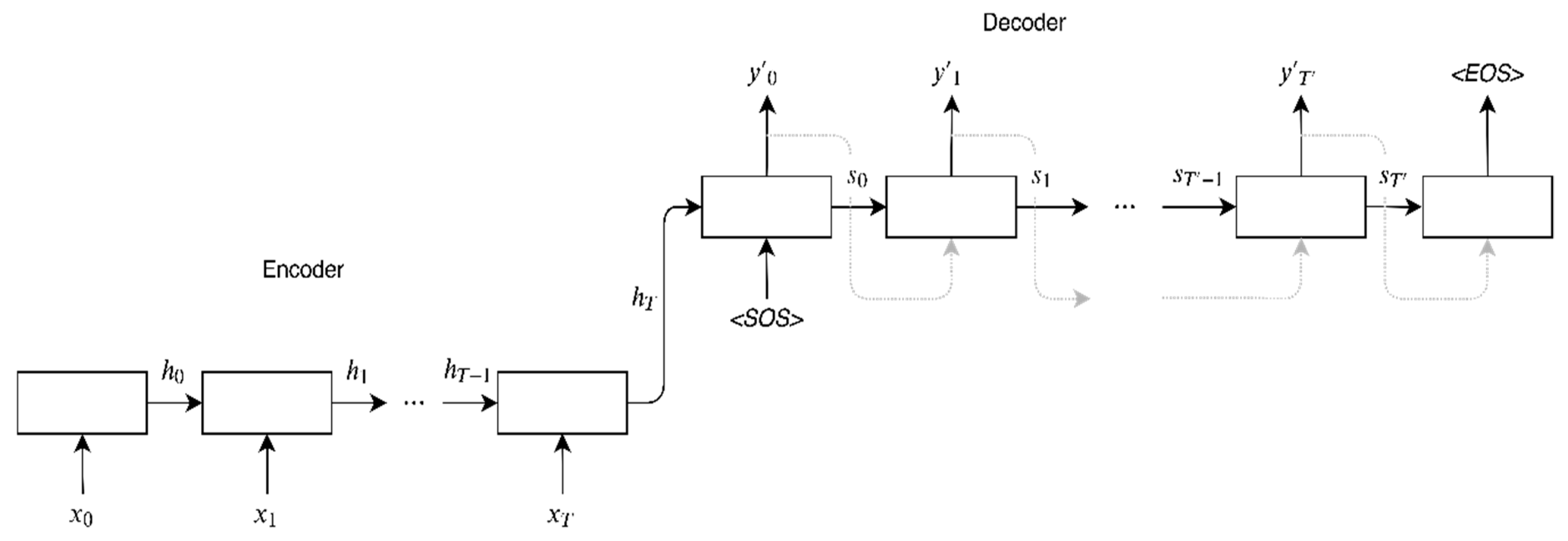
2.1. Sequence-To-Sequence (Seq2Seq) Encoder-Decoder Models

Firstly, we employed the idea of Sutskever et al. [39], who showed that that a straightforward approach using two connected RNNs can be used to solve general sequence-to-sequence problems. The main idea behind their proposed encoder-decoder model is to use RNN to read the input sequence, one step at a time, and use it to create a fixed-dimensional representation (context vector), that can be used by second RNN to generate an output sequence purely based on this vector representation. The encoder converts the input sequence X   =   ( x 1 ,   x 2 , x T ) and converts it to a context vector c using a set of hidden states of the RNN ( h 1 ,   h 2   h T ) :
h t   =   f ( x t ,   h t 1 ) ,
c   =   q   ( { ( h 1 ,   h 2   h T } ) ,
where h t R n is the hidden state calculated using input sequence element x t , q and f are non-linear function, for example RNNs.
The purpose of the decoder is to predict next element y t of the output sequence using context vector c and sequence of previously generated elements { y 1 ,   y 2 y t 1 } . In other words, the decoder defines a probability over generated output sequence Y   =   ( y 1 ,   y 2 , y T ) by decomposing the joint probability p ( Y ) into the ordered conditional probabilities:
p   ( Y )   =   t   =   1 T p ( y t | { y 1 ,   y 2 y t 1 } ,   c ) .
Each conditional probability can be evaluated using RNN:
p   ( y t | { y 1 ,   y 2 y t 1 } ,   c )   =   g   ( y t 1 ,   s t ,   c ) ,
where c is the context vector, s t is the hidden state of decoder RNN for the element t , g – non-linear function of RNN.
The graphical representation of a basic encoder-decoder model is given in Figure 1. The context vector is the last state of the encoder. Because these models are designed to work with variable length sequences, they use two special characters: the sequence start character <SOS> and the sequence end character <EOS>. The sequence start symbol is used as the start signal for the decoding part, and after the model generates the sequence end symbol <EOS>, the generation of further sequence elements is stopped. The entire input sequence is encoded into a single context vector, which is then used to generate the output sequence during decoding. With this solution, the models perform reasonably well when the input sequences are short, but do not perform well with the longer sequences.
The performance of a basic encoder-decoder models deteriorates rapidly as the length of the input sequence increases. This issue arises from the necessity to compress all information about the input sequence into one a fixed-length context vector. To overcome this issue, we experimented with an extension of a basic encoder–decoder model suggested by Bahdanau et al. [43] that can use all intermediate hidden states of an encoder to construct a context vector.

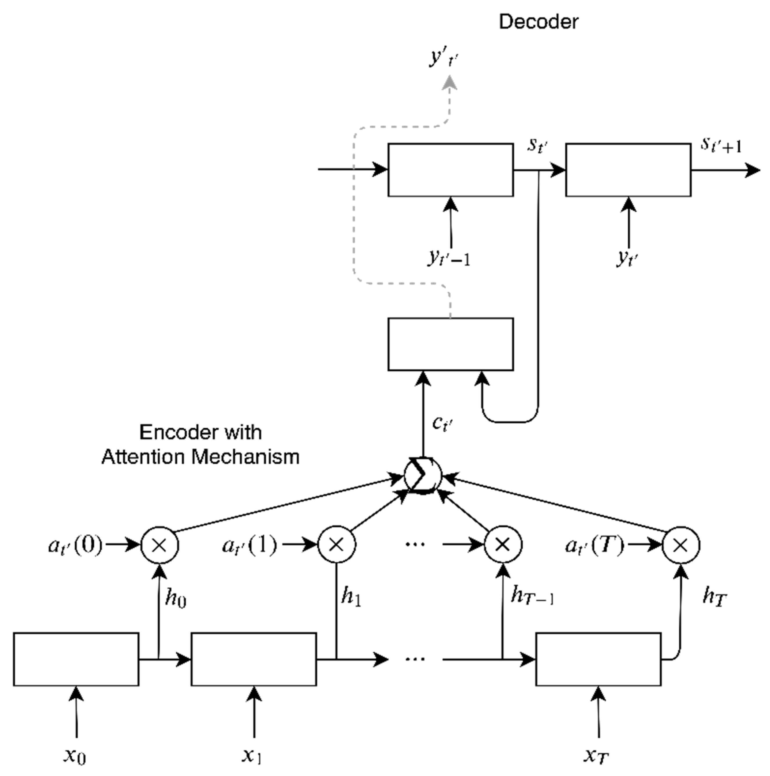
2.2. Attention Encoder–Decoder Models

Models with an attention mechanism attempt to solve the problem of working with longer sequences by allowing the decoder to “look back” into the input sequence at each step of the output sequence generation. Figure 2 demonstrates the operation of the attention mechanism. Models with an attention mechanism use weights a t to calculate the context vector. The number of weights depends on the number of output sequence elements and are calculated by comparing each decoder state s t with every hidden state of the encoder h t :
a t ( t )   =   e s c o r e ( s t ,   h t ) i   =   0 T 1 e s c o r e ( s t ,   h i ) ,
where T is the length of the input sequence, t is the index of the element in output sequence, and s c o r e is the scoring function. The most simplistic scoring function is just a dot product between two vectors:
s c o r e ( s t , h t )   =   s t h t .
Once the scoring vector is known, context vector c can be calculated using Equation (7), where T is the length of the input sequence and h t is the hidden state generated by processing element t of the input sequence:
c t   =   t   =   0 T a t h t .
The resulting context vector is concatenated with a hidden state h t from the decoder RNN, multiplied by weight matrix W c and processed using hyperbolic tangent function t a n h to calculate an updated hidden state h ˜ t (see Equation (8)), which in turn is used to calculate probability of next output symbol in the output sequence (Equation (9)):
h ˜ t   = t a n h ( W c [ c t ; h t ] )
p ( y t | { y 1 ,   y 2 y t 1 } ,   c )   =   s o f t m a x ( W s h ˜ t ) .
For training, the following loss function is used:
  =   t   =   0 T log p ( y t | y 1 , , y t 1 ,   X ) ,
where is the loss function,   X   =   ( x 1 , , x T ) is the sequence of phonems, Y   =   ( y 1 , , y T ) is the corresponding sequence of graphems.
During our experiments we have also investigated to what extent strategies proposed by other researchers, more specifically, training with reversed sequences [39] and using dropout [44] layer wise constructions [45], affects the performance of our models. For dropout, we used the following probability values proposed in [46] (the probability to keep the first layer neurons of encoder and decoder is 0.8; for hidden layer neurons, the probability is 0.5).

2.3. Computational Complexity Analysis

In practical use, the model prediction is generated by the RNN model. Following the recommendations of Xie et al. [47], the overall computation complexity of the proposed method consists of the four computation complexities of O ( 1 ) , O ( | C ε | ) ,   O ( | C ε | ) ,   and   O ( | C ε | ) .   The computation complexity of the loss function is O ( | C ε | ) . Note, however, that the element-wise multiplication, division, and log operation can be implemented in parallel with graphical parallel unit (GPU) at O ( 1 ) . In contrast, the implementation of CTC [48] based on a forward–backward algorithm has a computation complexity of O ( T · S ) , here S is the sequence length and T is the number of lokk-ahead steps.
As concerns the attention models, their computation complexity is directly proportional to the number of ‘attentions’. The computation complexity of the attention module itself is similar to that of CTC. Meanwhile, the attention mechanism requires the implementation of an additional module. Thus, its memory consumption is larger than that of CTC.

2.4. Evaluation of Models

For evaluation of the ASR system, we use accuracy (ACC), Levenshtein distance, and word error rate (WER) metrics.
Accuracy is calculated as:
A C C   =    T P + T N T P + T N + F P + F N   ,
where T P is the count of true positives, T N is the count of true negativess, F P is the count of false positives, F N is the count of false negatives.
Levenshtein distance is used to measure dissimilarity between two sequences made of symbols or words expressed in terms of the smallest number of edit operations (inserts, deletes, and replacements) required to perfectly match both sequences:
lev a , b ( i ,   j )   =   { max ( i ,   j ) i f   min ( i ,   j )   =   0 min { lev a , b ( i 1 ,   j ) + 1 lev a , b ( i ,   j 1 ) + 1 lev a , b ( i 1 ,   j 1 ) + 1 ( a i b j ) otherwise ,   ,
where lev a ,   b ( i ,   j ) is the edit distance between the first i symbols (words) of sequence a and the first j symbols (words) of sequence b ; 1 ( a i b j ) is a function that evaluates to 0 if a i   =   b j , and to 1, if a i   b j .
WER is calculated as follows:
W E R   =   S + I + D N ,
where S is the number of words recognized incorrectly, I is the number of words inserted by the ASR system, D is the number of words deleted by the system, and N is the total number of words.

3. Experiments and Results

3.1. Dataset

Speech corpus that we used to train and evaluate models contains 86 h of annotated Lithuanian speech (406 k words) from the Lithuanian speech corpora LIEPA [49]. It is composed of short commands, single word utterances, and even long sentences. There were 248 female and 128 male speakers, 83% of this group aged 15 to 22 yrs. The original phoneme system was MBROLA, all records were in 22 kHz, 16-bit mono format. The audio data were automatically processed to extract sequences of phonemes from raw audio files. Vocabularies of phonemes and graphemes consisted of 91 different phonemes and 61 distinct graphemes, respectively.
The characteristics of datasets by phoneme length used are summarized in Table 1. When measured by their phoneme sequence lengths most recordings are relatively short (<10 phonemes), although there are some very long recordings (up to 573 phonemes). The data in our corpus exhibits strong correlation between phoneme and grapheme sequence lengths (Pearson coefficient of 0.997), however not all sequence pairs have an equal length.
For our experiments, we split our corpus into 3 datasets: training dataset (60% of data, ~52 h of speech, 244,860 words), validation dataset (10% of data, ~26 h of speech, 40,841 words), and testing dataset (30% of data, ~9 h of speech, 120,387 words). We used the validation dataset to find the most appropriate hyperparameters and evaluated models on testing dataset to find how well these models generalize the unknown/unseen data.
To test to what extent encoder–decoder models can be used to perform automatic Lithuanian speech recognition, we decided to test selected models in isolated speech and long phrase recognition tasks.

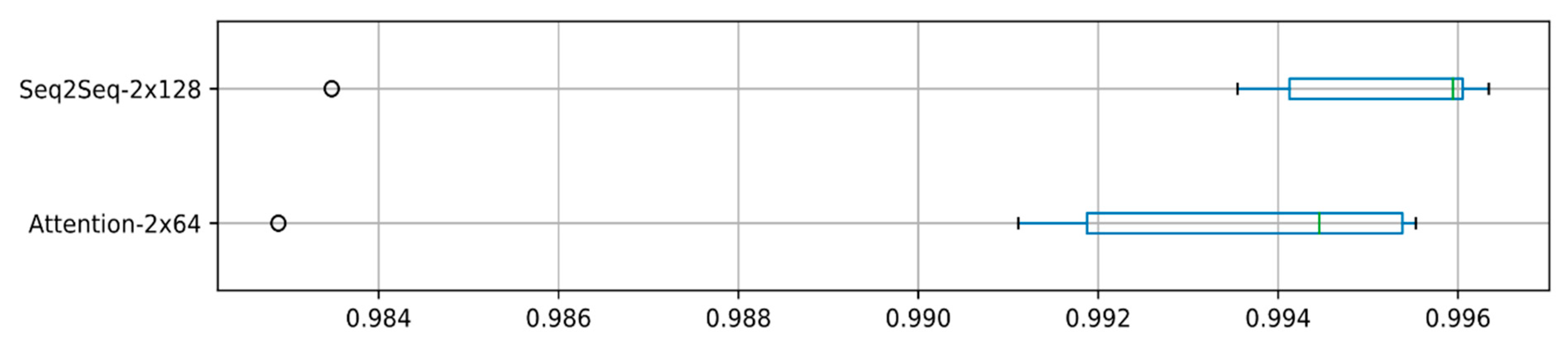
3.2. Isolated Speech Experiments

The first experiment was done to check if the models can find a mapping between phoneme sequences and their corresponding grapheme sequences. For this experiment we isolated every word (and its phoneme and grapheme sequences) in the training, validation, and testing datasets. We then trained our models using words from the training dataset and used the validation dataset to find the most appropriate hyperparameters. The models were trained using Adam optimization [50] with a learning rate of 0.01. To speed up training, we used the teacher-forcing method and applied a gradient clipping to keep the gradients of artificial neural networks between −5 and +5. We used batches of 32 sequences and made sure that all sequences were roughly the same length by bucketing sequences into buckets by their lengths, so that lengths of sequences in each bucket would not differ by more than 4. Finally, we used one-hot encoding to encode phonemes and graphemes as categorical variables.
To find the hyperparameters of the best performing model we tested several different configurations. More specifically, we trained 16 different models, which differed in the number of LSTM layers (from 2 to 5) and number of LSTM cells per layer (32, 64, 128, or 256).
The results of this experiment are presented in Table 2 and Table 3. We found that the best performing encoder–decoder model without attention mechanism had 2 LSTM layers with 128 LSTM cells per layer in encoder and decoder parts (Seq2Seq-2x128). Our best performing model with an attention mechanism had 2 LSTM layers with 64 bidirectional LSTM cells (Attention-2x64). Furthermore, we found, that when trained with reversed sequences, models perform slightly better. We have not found any benefits of using dropout even with deeper, wider networks.
The encoder–decoder models can learn to map phoneme sequences to their corresponding grapheme sequences, i.e., recognize uttered words solely from their phoneme sequences. Furthermore, it can achieve high recognition accuracy (>99%). Interestingly, we found that both the sequence–sequence and attention models behave similarly on all datasets.
To get a more accurate estimate of model performance and to ensure that our models do not suffer from sampling-bias, which may have occurred while splitting the original corpus into 3 datasets, we chose to train and test our models using 10-fold cross-validation. The cross-validation results, as presented in Figure 3, confirm that that both the Seq2Seq-2x128 and Attention-2x64 models can attain high accuracy (>99%). A relatively small spread around median accuracy proves that models do not overfit. Therefore, we claim that the encoder–decoder models generalize well and can learn to map phoneme sequences to grapheme sequences.
With the longer learning time of ANN, it can be seen that the loss function decreases steadily during the learning process, but the error with the verification dataset begins to increase over time. To avoid this, we use an early stopping strategy, which does not choose the final model parameters obtained at the end of the learning process, but the parameters with which the model has reached the minimum value of the loss function with the verification dataset.
We also evaluated the two best models using the Levenshtein distance metric (see Table 4). Low values of mean and median Levenshtein distance metric confirm that the Seq2Seq-2x128 and Attention-2x64 models can recognize words well and the errors are rare.

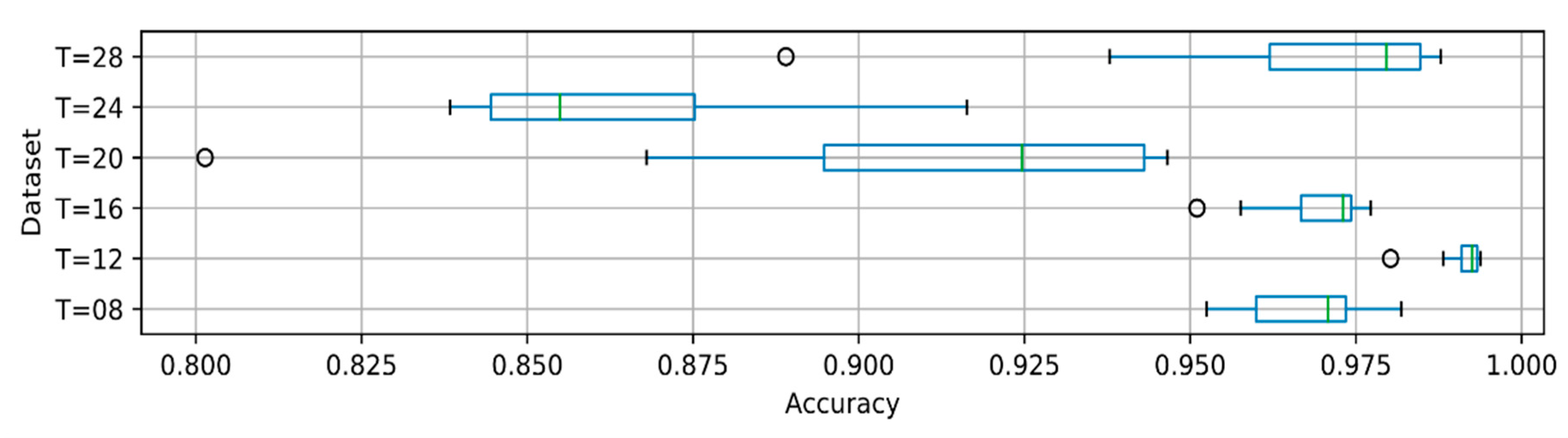
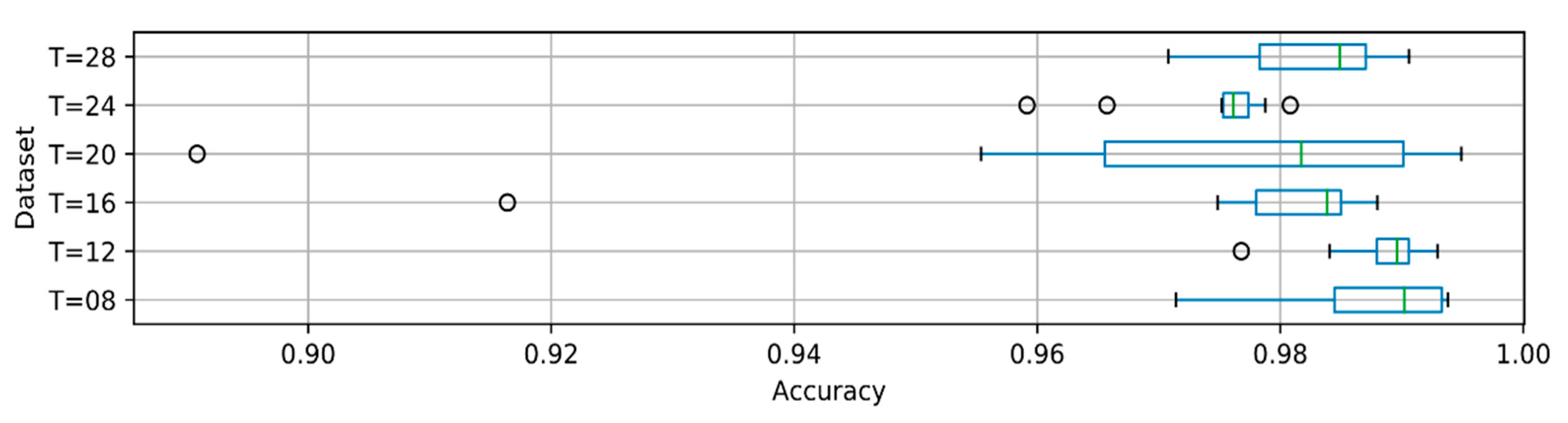
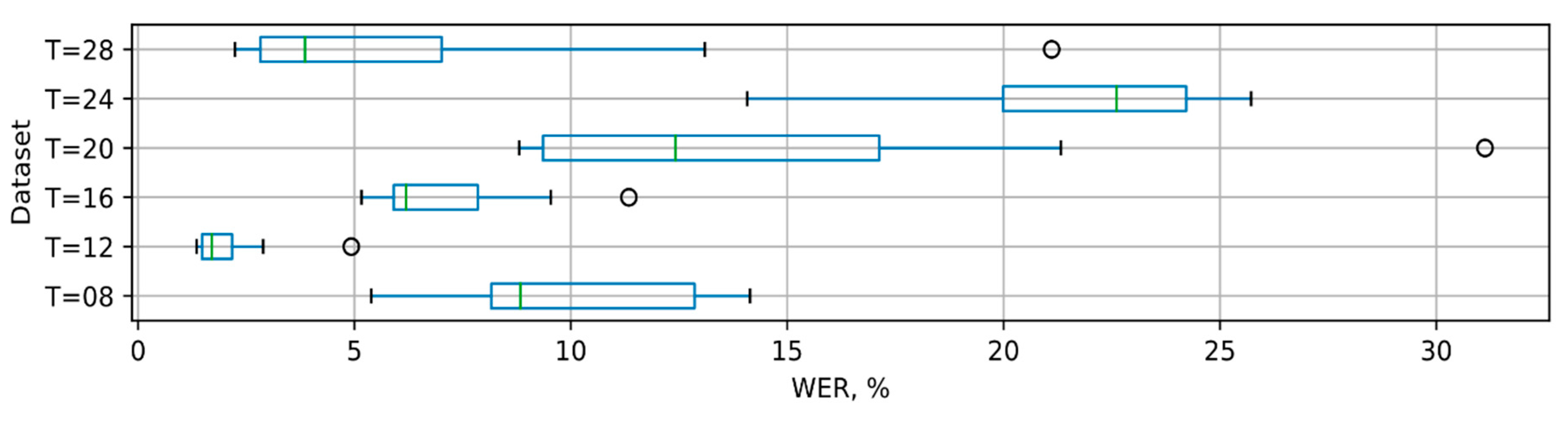
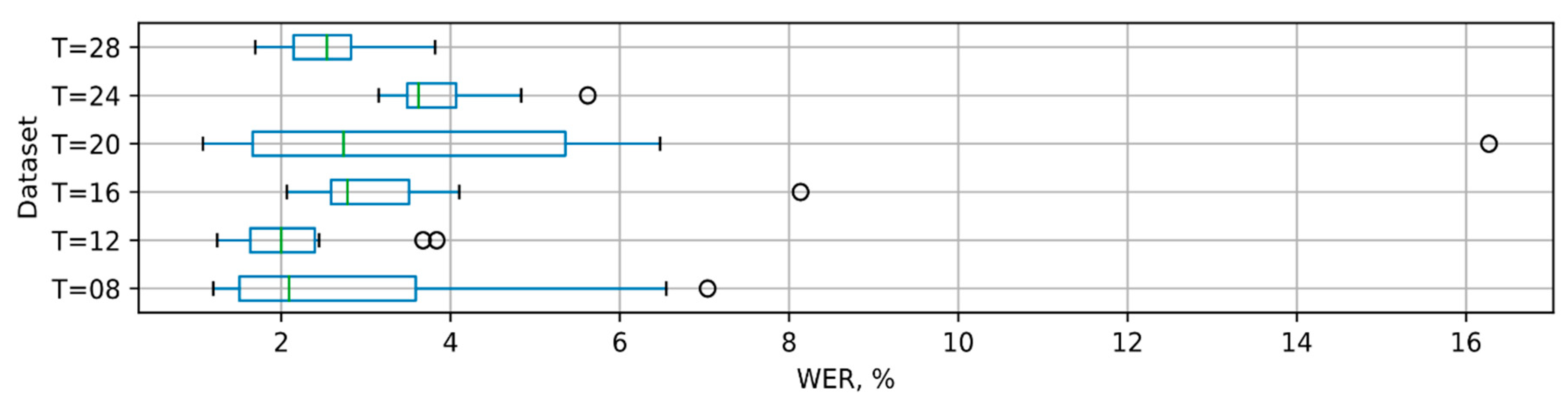
3.3. Recognition of Long Phrases

The second experiment was performed to investigate how well these models could be applied to recognition of long phrases. This is a much more demanding task, as it requires the model not only to learn a mapping between phoneme and grapheme sequences, but also to be able to distinguish which part of a phoneme sequence belongs to which word, i.e., to find beginnings and endings of the words. For this experiment, we sampled sequences from the original datasets by taking every combination of consecutive words in the recording, for example, in an utterance of 3 words ( α , β , γ ) we created 6 different sequences: ( α ) , ( β ) ,   ( γ ) ,   ( α , β ) ,   ( β , γ ) ,   ( α , β , γ ) . The phoneme and grapheme sequences corresponding to these words were merged together. The spaces were added to the grapheme sequences to mark the word boundaries. The resulting sequences were filtered by their lengths to create 6 different dataset groups. Each dataset group was bounded by the longest sequence of phoneme in that group.
We used models from previous experiment (Seq2Seq-2x128 and Attention-2x64) and trained them on each dataset group in order to find (a) whether models can learn to distinguish words when there is more than one word in the utterance; (b) how sequence length affects performance of our models. As in the previous experiment, we used the Adam optimization, however, this time we lowered the learning rate to 0.001. We trained our models using reversed sequences and clipped the gradients using threshold −5 and +5. Each model was trained for 20 epochs with early stopping.
The results of our experiment are presented in Table 5 and Table 6. Table 5 shows that models can achieve high accuracy even when trained with phoneme sequences from multiple words. The best accuracy was achieved by Seq2Seq-2x128 (0.990) and Attention-2x64 (0.992).
Table 6 indicates that models can reach very low WER values. Interestingly, few configurations (e.g., Seq2Seq-2x128 model was trained with dataset, where the longest phoneme sequence is 28 phonemes long, while Attention-2x64 model was trained with the longest phoneme sequence of 20 phonemes) show very large differences between validation and testing accuracy metrics. The same pattern can be observed in the WER results.
Our results indicate that models cannot only map phonemes to corresponding sequences of graphemes, but also learn to find word boundaries and distinguish words in these sequences. The encoder–decoder models can be used as a viable option for speech recognition from phone sequences.
Interestingly, we can observe that the models trained on a dataset, where the longest phoneme sequence is just 8 phonemes, perform much worse than the models which were trained with longer sequences. While it is unclear, what causes models to underperform with short sequences, we speculate that this might be due to a much smaller training dataset.
As with isolated speech experiments, we tested the performance of our models using 10-fold cross-validation. The cross-validation results are presented in Figure 4 and Figure 5.
By comparing Seq2Seq-2x128 and Attention-2x64 results, we can see that the model with an attention mechanism (Attention-2x64) is much more stable with both shorter and longer sequences, as high recognition accuracy was achieved on almost all folds. The basic sequence–sequence encoder–decoder model, on the other hand, does not perform as well as the model with attention mechanism, and the results of each fold have more variability, as indicated by a larger interquartile range (see, e.g., sequences of T = 20 and T = 24).
The WERs, of which models managed to achieve during cross-validation, are presented in Figure 6 and Figure 7. It is apparent that the Seq2Seq-2x128 model is less stable, as compared to the attention-2x64 model with an attention mechanism, as indicated by higher interquartile range.
While in our experiments we limited phoneme sequences to 28 phonemes, we believe that larger encoder–decoder models can be used with even longer sequences.

4. Discussion

Although the field of automatic Lithuanian language recognition is not new, there are few ASR applications and related research in the field of Lithuanian language processing. The main reasons are the complexity of the Lithuanian language and the lack of linguistic data. The Lithuanian language has a complex pronunciation, a flexible word order and a rich vocabulary, while the spelling is supplemented with the Latin alphabet. Analyzing and comparing existing systems, solutions, and comparisons is not easy—the Lithuanian speech recognition systems differ not only in datasets used for training (phoneme formats, record quantities, their contents, etc.), but also in recognition methodologies and purposes used (some systems are limited to phoneme recognition in acoustic signals, others are able to work on recognizing individual words as well).
Our algorithm provides a major impact in the implementation: The method does not require any heuristic loss functions, explicit phonetic representations, or assumptions of conditional independence, as in more traditional approaches. In classical automatic speech recognition systems, such phoneme sequence recognition is performed using a consonant pattern (dictionary), which allows words to be recognized by their phoneme sequences, and the resulting words are refined by the speech model during the decoding step. Building pronunciation and language models is a complex and lengthy process, especially for morphologically rich languages, and the resulting models do not guarantee good results for the ASR system. On the other hand, in speech recognition systems that perform the recognition from the beginning to the end of a signal unit, the concept of phonemes does not even exist because of their latent representation in the model.
Another positive impact is provided in the actual cost of resources needed to train the system (especially in comparison to the classic, HMM-based solutions), also in the partially simplified and easier to assemble language model (defined by our network structure), proving that it is possible to reach a usable recognition accuracy for languages with little, publicly available linguistic resources. Our method proves that a positive impact could be seen on most transcription-based operations, often typically consisting of long phrases. ASR systems such as the system proposed in this paper are based on the phoneme sequences processing, which is simpler than classical speech recognition systems and has the flexibility to use pre-existing acoustic models. Learning to use the phoneme sequences allows the ASR system to master not only the relationship between the graphemes and their corresponding phonemes or groups, but also to learn how to distinguish between individual words, i.e., to form a language model. The close relationship between phonetic and morphological forms of words in Lithuanian allow the proposed ASR system to achieve high speech recognition results.
Summarizing the results obtained during the experiment, it can be stated that the encoded–decoder-type models can effectively learn the relationship between phonemes and their corresponding grapheme sequences and can achieve very good results in the problem of automatic recognition of isolated words from Lithuanian phoneme sequences.

5. Conclusions

We have demonstrated that the encoder–decoder models can be used to perform automatic Lithuanian speech recognition by learning the mapping between phonemes and corresponding sequences of graphemes. The experimental results indicate that both the basic encoder–decoder model and a more advanced model with an attention mechanism can learn to accurately predict spoken words purely from their phonetic forms with a very high accuracy (up to 0.96).
We demonstrated that these types of models can be applied not only to isolated speech recognition tasks, but also to recognition of long phrases, as they can learn to distinguish words in longer sequences by finding their boundaries (0.998 accuracy achieved with sequences consisting of 28 phonemes). Our results suggest that the model can be successful with even longer sequences.
Compared to the performance of the Lithuanian language Google speech recognizer on the same LIEPA corpora [51], this solution was on average around 30% more efficient.
In the future, we will also apply the proposed approach for other languages, which have strong ties between the phonetic and morphological forms of the words.

Author Contributions

Conceptualization, R.M.; formal analysis, R.M.; investigation, L.P.; methodology, R.M.; resources, L.P.; software, L.P.; supervision, R.M.; validation, L.P. and R.M.; writing—original draft, L.P. and R.M.; writing—review & editing, R.D.

Funding

This research received no external funding.

Conflicts of Interest

The authors declare no conflict of interest.

References

  1. Badenhorst, J.; de Wet, F. The Usefulness of Imperfect Speech Data for ASR Development in Low-Resource Languages. Information 2019, 10, 268. [Google Scholar] [CrossRef]
  2. Nassif, A.B.; Shahin, I.; Attili, I.; Azzeh, M.; Shaalan, K. Speech recognition using deep neural networks: A systematic review. IEEE Access 2019, 7, 19143–19165. [Google Scholar] [CrossRef]
  3. Wang, D.; Wang, X.; Lv, S. End-to-End Mandarin Speech Recognition Combining CNN and BLSTM. Symmetry 2019, 11, 644. [Google Scholar] [CrossRef]
  4. Panayotov, V.; Chen, G.; Povey, D.; Khudanpur, S. Librispeech: An ASR corpus based on public domain audio books. In Proceedings of the 2015 IEEE International Conference on Acoustics, Speech and Signal Processing (ICASSP), South Brisbane, Australia, 19–24 April 2015; pp. 5206–5210. [Google Scholar]
  5. Bu, H.; Du, J.; Na, X.; Wu, B.; Zheng, H. AIShell-1: An open-source Mandarin speech corpus and a speech recognition baseline. In Proceedings of the 20th Conference of the Oriental Chapter of the International Coordinating Committee on Speech Databases and Speech I/O Systems and Assessment (O-COCOSDA), Seoul, Korea, 1–3 November 2017; pp. 1–5. [Google Scholar]
  6. Watanabe, S.; Hori, T.; Karita, S.; Hayashi, T.; Nishitoba, J.; Unno, Y.; Soplin, N.E.Y.; Heymann, J.; Wiesner, M.; Chen, N.; et al. ESPnet: End-to-End Speech Processing Toolkit. arXiv 2018, arXiv:1804.00015. [Google Scholar] [Green Version]
  7. Tamazin, M.; Gouda, A.; Khedr, M. Enhanced Automatic Speech Recognition System Based on Enhancing Power-Normalized Cepstral Coefficients. Appl. Sci. 2019, 9, 2166. [Google Scholar] [CrossRef]
  8. Besacier, L.; Barnard, E.; Karpov, A.; Schultz, T. Automatic speech recognition for under-resourced languages: A survey. Speech Commun. 2014, 56, 85–100. [Google Scholar] [CrossRef]
  9. Zhang, Z.; Geiger, J.; Pohjalainen, J.; Mousa, A.E.; Jin, W.; Schuller, B. Deep learning for environmentally robust speech recognition: An overview of recent developments. ACM Trans. Intell. Syst. Technol. 2018, 9. [Google Scholar] [CrossRef]
  10. Yu, C.; Chen, Y.; Li, Y.; Kang, M.; Xu, S.; Liu, X. Cross-Language End-to-End Speech Recognition Research Based on Transfer Learning for the Low-Resource Tujia Language. Symmetry 2019, 11, 179. [Google Scholar] [CrossRef]
  11. Lipeika, A.; Lipeikienė, J.; Telksnys, L. Development of Isolated Word Speech Recognition System. Informatica 2002, 13, 37–46. [Google Scholar]
  12. Raškinis, G.; Raškinienė, D. Building Medium-Vocabulary Isolated-Word Lithuanian HMM Speech Recognition System. Informatica 2003, 14, 75–84. [Google Scholar]
  13. Filipovič, M.; Lipeika, A. Development of HMM/Neural Network-Based Medium-Vocabulary Isolated-Word Lithuanian Speech Recognition System. Informatica 2004, 15, 465–474. [Google Scholar]
  14. Dovydaitis, L.; Rudžionis, V. Identifying Lithuanian native speakers using voice recognition. In Business Information Systems Workshops; Springer International Publishing: Berlin, Germany, 2017; pp. 79–84. [Google Scholar]
  15. Ivanovas, E.; Navakauskas, D. Towards speaker identification system based on dynamic neural network. Electron. Electr. Eng. 2012, 18, 69–72. [Google Scholar] [CrossRef]
  16. Korvel, G.; Treigys, P.; Tamulevičius, G.; Bernatavičienė, J.; Kostek, B. Analysis of 2D feature spaces for deep learning-based speech recognition. AES J. Audio Eng. Soc. 2018, 66, 1072–1081. [Google Scholar] [CrossRef]
  17. Salimbajevs, A.; Kapociute-Dzikiene, J. General-Purpose Lithuanian Automatic Speech Recognition System. In Proceedings of the 8th International Conference, Baltic HLT, Tartu, Estonia, 27–29 September 2018; pp. 150–157. [Google Scholar]
  18. Povey, D.; Peddinti, V.; Galvez, D.; Ghahremani, P.; Manohar, V.; Na, X.; Wang, Y.; Khudanpur, S. Purely Sequence-Trained Neural Networks for ASR Based on Lattice-Free MMI. In Proceedings of the Interspeech, San Francisco, CA, USA, 8–12 September 2016; pp. 2751–2755. [Google Scholar]
  19. Yajie, M.; Zhang, H.; Metze, F. Towards speaker adaptive training of deep neural network acoustic models. In Proceedings of the Fifteenth Annual Conference of the International Speech Communication Association, Singapore, 14–18 September 2014. [Google Scholar]
  20. Šilingas, D.; Laurinčiukaitė, S.; Telksnys, L. Towards Acoustic Modeling of Lithuanian Speech. In Proceedings of the 2004 International Conference on Speech and Computer (SPECOM), Saint-Petersburg, Russia, 20–22 September 2004; pp. 326–333. [Google Scholar]
  21. Lipeika, A.; Laurinčiukaitė, S. Framework for Choosing a Set of Syllables and Phonemes for Lithuanian Speech Recognition. Informatica 2007, 18, 395–406. [Google Scholar]
  22. Laurinčiukaitė, S.; Lipeika, A. Syllable-Phoneme based Continuous Speech Recognition. Electr. Eng. 2006, 6, 10–13. [Google Scholar]
  23. Lileikyte, R.; Gorin, A.; Lamel, L.; Gauvain, J.L.; Fraga-Silva, T. Lithuanian Broadcast Speech Transcription Using Semi-supervised Acoustic Model Training. Proc. Comput. Sci. 2016, 81, 107–113. [Google Scholar] [CrossRef] [Green Version]
  24. Alumäe, T.; Tilk, O. Automatic speech recognition system for Lithuanian broadcast audio. Front. Artif. Intell. Appl. 2016, 289, 39–45. [Google Scholar] [CrossRef]
  25. Lileikytė, R.; Lamel, L.; Gauvain, J.-L.; Gorin, A. Conversational telephone speech recognition for Lithuanian. Comput. Speech Lang. 2018, 49, 71–82. [Google Scholar] [CrossRef]
  26. Gales, M.J.F.; Knill, K.M.; Ragni, A. Unicode-based graphemic systems for limited resource languages. In Proceedings of the 2015 IEEE International Conference on Acoustics, Speech and Signal Processing (ICASSP), Brisbane, QLD, Australia, 19–24 April 2015; pp. 5186–5190. [Google Scholar]
  27. Maskeliunas, R.; Rudžionis, A.; Ratkevičius, K.; Rudžionis, V. Investigation of foreign languages models for lithuanian speech recognition. Electron. Electr. Eng. 2009, 3, 15–20. [Google Scholar]
  28. Rudzionis, V.; Maskeliunas, R.; Rudzionis, A.; Ratkevicius, K. On the adaptation of foreign language speech recognition engines for Lithuanian speech recognition. Lect. Notes Bus. Inf. Process 2009, 37, 113–118. [Google Scholar] [CrossRef]
  29. Rudzionis, V.; Raskinis, G.; Maskeliunas, R.; Rudzionis, A.; Ratkevicius, K. Comparative analysis of adapted foreign language and native Lithuanian speech recognizers for voice user interface. Electron. Electr. Eng. 2013, 19, 90–93. [Google Scholar] [CrossRef]
  30. Rasymas, T.; Rudžionis, V. Combining multiple foreign language speech recognizers by using neural networks. Front. Artif. Intell. Appl. 2014, 268, 33–39. [Google Scholar] [CrossRef]
  31. Rudzionis, A.; Rudzionis, V. Phoneme recognition in fixed context using regularized discriminant analysis. In Proceedings of the Sixth European Conference on Speech Communication and Technology (EUROSPEECH’99), Budapest, Hungary, 5–9 September 1999. [Google Scholar]
  32. Driaunys, K.; Rudžionis, V.; Žvinys, P. Averaged Templates Calculation and Phoneme Classification. Inf. Technol. Control. 2007, 36. [Google Scholar] [CrossRef]
  33. Rudzionis, A.; Rudzionis, V. Lithuanian Speech Database LTDIGITS. In Proceedings of the Third International Conference on Language Resources and Evaluation (LREC’02), Las Palmas, Canary Islands, Spain, 29–31 May 2002. [Google Scholar]
  34. Vaičiūnas, A.; Kaminskas, V.; Raskinis, G. Statistical Language Models of Lithuanian Based on Word Clustering and Morphological Decomposition. Informatica 2004, 15, 565–580. [Google Scholar]
  35. Karpov, A.; Markov, K.; Kipyatkova, I.; Vazhenina, D.; Ronzhin, A. Large vocabulary Russian speech recognition using syntactico-statistical language modeling. Speech Commun. 2014, 56, 213–228. [Google Scholar] [CrossRef]
  36. Kipyatkova, I.S.; Karpov, A.A. A study of neural network Russian language models for automatic continuous speech recognition systems. Autom. Remote Control 2017, 78, 858–867. [Google Scholar] [CrossRef]
  37. Jadczyk, T. Audio-visual speech-processing system for Polish applicable to human-computer interaction. Comput. Sci. 2018, 19, 41–64. [Google Scholar] [CrossRef]
  38. Pakoci, E.; Popović, B.; Pekar, D. Improvements in Serbian speech recognition using sequence-trained deep neural networks. SPIIRAS Proc. 2018, 3, 53–76. [Google Scholar] [CrossRef]
  39. Sutskever, I.; Vinyals, O.; Le, Q.V. Sequence to sequence learning with neural networks. In Proceedings of the Advances in Neural Information Processing Systems 27 (NIPS 2014), Montreal, Canada, 8–13 December 2014; pp. 3104–3112. [Google Scholar]
  40. Luong, M.-T.; Pham, H.; Manning, C.D. Effective Approaches to Attention-based Neural Machine Translation. arXiv 2015, arXiv:1508.04025. [Google Scholar] [Green Version]
  41. Fayek, H.M.; Lech, M.; Cavedon, L. Evaluating deep learning architectures for Speech Emotion Recognition. Neur. Netw. 2017, 92, 60–68. [Google Scholar] [CrossRef]
  42. Hannun, A. Sequence Modeling with CTC. Distill 2017, 2. [Google Scholar] [CrossRef]
  43. Bahdanau, D.; Cho, K.; Bengio, Y. Neural Machine Translation by Jointly Learning to Align and Translate. Proceedings of International Conference on Learning Representations (ICLR), San Diego, CA, USA, 8–9 May 2015. [Google Scholar]
  44. Srivastava, N.; Hinton, G.; Krizhevsky, A.; Sutskever, I.; Salakhutdinov, R. Dropout: A simple way to prevent neural networks from overfitting. J. Mach. Learn. Res. 2014, 15, 1929–1958. [Google Scholar]
  45. Zeyer, A.; Doetsch, P.; Voigtlaender, P.; Schluter, R.; Ney, H. A comprehensive study of deep bidirectional LSTM RNNS for acoustic modeling in speech recognition. In Proceedings of the 2017 IEEE International Conference on Acoustics, Speech and Signal Processing (ICASSP), New Orleans, LA, USA, 5–9 March 2017. [Google Scholar]
  46. Goodfellow, I.; Bengio, Y.; Courville, A. Deep Learning; MIT Press: Cambridge, MA, USA, 2016. [Google Scholar]
  47. Xie, Z.; Huang, Y.; Zhu, Y.; Jin, L.; Liu, Y.; Xie, L. Aggregation Cross-Entropy for Sequence Recognition. In Proceedings of the IEEE Conference on Computer Vision and Pattern Recognition, CVPR 2019, Long Beach, CA, USA, 16–20 June 2019; pp. 6538–6547. [Google Scholar]
  48. Graves, A. Supervised Sequence Labelling; Springer: Berlin, Germany, 2012. [Google Scholar]
  49. Liepa Corpora. Interactive Repository Link. Available online: https://www.xn--ratija-ckb.lt/liepa (accessed on 17 October 2019).
  50. Kingma, D.; Ba, J. Adam: A method for stochastic optimization. arXiv 2014, arXiv:1412.6980. [Google Scholar]
  51. Sipavičius, D.; Maskeliūnas, R. “Google” Lithuanian Speech Recognition Efficiency Evaluation Research. In Proceedings of the International Conference on Information and Software Technologies, Druskininkai, Lithuania, 13–15 October 2016; pp. 602–612. [Google Scholar]
Figure 1. Adapted encoder-decoder model.
Computers 08 00076 g001
Figure 2. Encoder–decoder model with attention mechanism.
Computers 08 00076 g002
Figure 3. Accuracy of k-fold cross-validation results with isolated speech dataset.
Computers 08 00076 g003
Figure 4. Seq2Seq-2x128 cross-validation results.
Computers 08 00076 g004
Figure 5. Attention-2x64 cross-validation results.
Computers 08 00076 g005
Figure 6. WER graph of Seq2Seq-2x128 cross-validation results.
Computers 08 00076 g006
Figure 7. WER graph of Attention-2x64 cross-validation results.
Computers 08 00076 g007
Table 1. Statistical characteristics of the dataset.
Max Length of PhonemesT = 8T = 12T = 16T = 20T = 24T = 28
Number of words417,935765,8451,273,9831,821,4392,473,0733,151,933
Number of sequences367,989570,321782,68096,52111,145,0861,304,801
Table 2. Results of experiments with isolated words dataset using Seq2Seq models (best values are shown in bold).
ModelNumber of Hidden LayersNumber of Epochs TrainedTraining LossTraining AccuracyTesting LossTesting Accuracy
Seq2Seq-2x32281.7090.9910.7020.976
Seq2Seq-2x642101.7030.9940.6250.986
Seq2Seq-2x128291.7010.9950.5340.991
Seq2Seq-2x256231.7110.9900.7030.973
Seq2Seq-3x32381.7130.9890.7140.960
Seq2Seq-3x643101.7090.9910.5960.982
Seq2Seq-3x128391.7110.9900.6120.978
Seq2Seq-3x2563101.7850.9542.3500.778
Seq2Seq-4x32481.7700.9640.9950.897
Seq2Seq-4x644101.7830.9552.0470.810
Seq2Seq-4x128471.7320.9800.9400.939
Seq2Seq-4x256481.9660.8124.0410.451
Seq2Seq-5x32581.7450.9740.9890.920
Seq2Seq-5x64571.8060.9431.6570.812
Seq2Seq-5x128572.1750.6856.8320.217
Seq2Seq-5x256573.1530.1722.9390.180
Table 3. Results of experiments with isolated words dataset using attention models (best values are shown in bold).
ModelNumber of Hidden LayersNumber of Epochs TrainedTraining LossTraining AccuracyTesting LossTesting Accuracy
Attention-2x32281.7010.9940.5520.989
Attention-2x64221.7100.9900.5140.993
Attention-2x128211.7590.9590.5300.989
Attention-2x256212.4380.6547.1130.111
Attention-3x32351.7030.9940.5270.985
Attention-3x64331.7070.9920.5380.988
Attention-3x128311.7870.9420.5230.990
Attention-3x256351.8320.9590.6910.969
Attention-4x32461.7020.9940.6050.965
Attention-4x64461.7060.9920.8200.949
Attention-4x128441.7110.9900.5080.990
Attention-4x256443.1700.3112.5230.302
Attention-5x32561.7070.9920.6300.967
Attention-5x64551.7060.9920.6080.976
Attention-5x128531.7500.9730.7970.921
Attention-5x256552.5880.4962.2970.457
Table 4. Comparison of two best models on the testing dataset.
ModelLoss ValueAccuracyMean LevenshteinMedian Levenshtein
Seq2Seq-2x1280.5360.9910.0430
Attention-2x640.5150.9930.0280
Table 5. Results of the experiments with long phrase dataset (best values are shown in bold).
ModelLongest Phoneme Sequence in the DatasetNumber of Epochs TrainedTraining AccuracyValidation AccuracyTest Accuracy
Seq2Seq-2x1288180.9960.9920.875
Seq2Seq-2x12812190.9970.9220.920
Seq2Seq-2x12816190.9970.9820.985
Seq2Seq-2x12820130.9970.9660.960
Seq2Seq-2x12824200.9980.9560.953
Seq2Seq-2x12828200.9980.8490.990
Attention-2x648160.9960.9140.858
Attention-2x6412190.9970.9750.975
Attention-2x6416200.9980.9630.951
Attention-2x6420170.9980.9930.992
Attention-2x6424180.9980.9300.874
Attention-2x6428200.9990.9930.988
Table 6. Word error rate (WER) of the experiments with long phrase dataset (best values are shown in bold).
ModelLongest Phoneme Sequence in the DatasetValidation WERTest WER
Seq2Seq-2x12882.08624.692
Seq2Seq-2x1281213.95314.057
Seq2Seq-2x128162.9052.394
Seq2Seq-2x128205.0975.693
Seq2Seq-2x128246.1426.362
Seq2Seq-2x1282820.0391.524
Attention-2x64810.40620.887
Attention-2x64123.1043.150
Attention-2x64164.0715.239
Attention-2x64201.0871.303
Attention-2x64247.09812.989
Attention-2x64281.0981.583

