Semantic Features for Optimizing Supervised Approach of Sentiment Analysis on Product Reviews

Abstract

The growth of ecommerce has triggered online reviews as a rich source of product information. Revealing consumer sentiment from the reviews through Sentiment Analysis (SA) is an important task of online product review analysis. Two popular approaches of SA are the supervised approach and the lexicon-based approach. In supervised approach, the employed machine learning (ML) algorithm is not the only one to influence the results of SA. The utilized text features also handle an important role in determining the performance of SA tasks. In this regard, we proposed a method to extract text features that takes into account semantic of words. We argue that this semantic feature is capable of augmenting the results of supervised SA tasks compared to commonly utilized features, i.e., bag-of-words (BoW). To extract the features, we assigned the correct sense of the word in reviewing the sentence by adopting a Word Sense Disambiguation (WSD) technique. Several WordNet similarity algorithms were involved, and correct sentiment values were assigned to words. Accordingly, we generated text features for product review documents. To evaluate the performance of our text features in the supervised approach, we conducted experiments using several ML algorithms and feature selection methods. The results of the experiments using 10-fold cross-validation indicated that our proposed semantic features favorably increased the performance of SA by 10.9%, 9.2%, and 10.6% of precision, recall, and F-Measure, respectively, compared with baseline methods.

1. Introduction

With the rapid growth of ecommerce platforms for online shopping, more and more customers share their opinions about products on the internet. This fact has generated a huge amount of opinion data within the platform [1]. The opinion data has then emerged as a valuable and objective source of product information for both customers and companies. For customers, it helps them by recommending that they buy a certain product [2]. For companies, it can help them in evaluating the design of a product [3] based on the analysis of user generated content (UGC), i.e., product reviews describing the user’s experience [4]. With the quantity of the data, manual processing is not an efficient task. Alternatively, a big data analytics technique is necessary [5]. Sentiment Analysis (SA) has arisen in response to the necessity of processing the huge data in speed [6]. SA is a computational technique to automate the extraction of subjective information, i.e., opinion of customers with respect to a product [7]. For that reason, this study is important.

One of the most popular methods employed for SA tasks is the machine learning (ML)-based method [8], i.e., a supervised approach employing an ML algorithm. Although the role of the ML algorithm is important, it is not yet the only factor that determines the performance of SA. As a text classification task, another important factor influencing the SA result is the employed text features [9]. Semantic features are considered important for augmenting the result of SA tasks [10] by providing correct sense of a word according to its local context, i.e., sentence. Providing the correct sense of words means providing correct sentiment value that is important in extracting a robust feature set for supervised SA. The best we know, recent lexicon based approaches of SA studies that concern semantics of words, like the work of [11] and [10], have not been evaluated in a supervised environment.

Saif [11] has considered semantics of words by proposing a method called Contextual Semantics. The study introduced SentiCircle, which adheres to the distributional hypothesis that words that appear in similar contexts share identical meanings. This method has outperformed baseline methods when experimented and evaluated in several different sentiment lexicons, i.e., SentiWordNet [12], Multi-Perspective Question Answering (MPQA) subjectivity lexicon [13], and Thelwall-Lexicon [14] using several Twitter datasets, i.e., Obama McCain Debate (OMD), Health Care Reform (HCR), and Stanford Sentiment Gold Standard (STS-Gold).

Another work, [10], has also concerned semantic of words. The study provided extension for [11] by assigning prior sentiment value based on the context of the word using a graph-based Word Sense Disambiguation (WSD) technique. The work has also introduced a similarity-based technique to determine pivot words used in [11]. Tested in several product review domains, i.e., automotive, beauty, books, electronics, and movies, the result of this study has outperformed baselines in several performance metrics, i.e., precision, recall, and F-Measure. The result of [11] and [10] have highlighted the importance of semantics in SA tasks.

Meanwhile, other studies using the supervised approach commonly utilize the bag-of-words (BoW) feature or its extension as the base of the classification task. In this paper, we extend the previous lexicon-based approach presented in [10] to generate a set of sentiment features that is capable of capturing the semantics of words. The feature set was evaluated in a supervised environment.

Referring to the previously described research gap, the purposes for this study comprised:

• Augmenting the results of supervised SA tasks for online product reviews by proposing a method for extracting sentiment features that takes into account semantics of words. The proposed method is the extension of [10].
• Evaluating the semantic features in various ML algorithms and feature selection methods.
• Finding the best set of the features using several feature selection methods.

In assigning the correct sense of the words in a review sentence, an adapted WSD method was used. In this method, the sense is picked from the WordNet lexical database. To calculate the numeric value of the feature, one of three sentiment values of the sense, i.e., positivity, negativity, and objectivity, is then picked from the SentiWordNet database [12]. Employing several WordNet similarity algorithms, we present a method to generate a semantic feature set of words. To evaluate the performance of our proposed semantic features, several ML algorithms and feature selection methods were employed. The employed ML algorithms and feature selection methods are implemented in WEKA, an open source tool containing algorithms for data mining applications [15]. The results of these experiments using 10-fold cross-validation indicated that our proposed semantic features favorably enhanced the performance of SA in terms of precision, recall, and F-Measure. The rest of this manuscript is organized in the following sections. Section 2 explores the most recent related study that has previously been done. Section 3 describes the method for extracting semantic features of words, including the formulas that are introduced. We explain the scenario of the experiments and the results in Section 4. The results of the experiments are discussed in Section 4. Finally, we highlight the effectiveness of our proposed method in Section 5.

2. Related Work

The expansion of online shopping has triggered consumer to express their opinion about a product they have purchased on ecommerce platform. SA is an efficient text mining technique to extract the opinion from online product reviews [16]. Two types of approaches that is commonly employed to perform SA task, i.e., supervised approach and lexicon based approach [17]. Supervised approaches make use of labeled training data to learn the model. Using an ML algorithm, the model is then performed to test the dataset. Using Hybrid ML approach, Al Amrani [18] performed SA on an Amazon review dataset. A number of decision trees at randomly selected features were firstly picked to forecast the class of test dataset. Support Vector Machine (SVM) was then used to maximize the margin that separates two classes. Since RF was not sensitive to input, the default parameters were used for each classifier. The method was applied to the Amazon review dataset.

To optimize the SA task, Singh [19] employed four ML classifiers, i.e., Naïve Bayes, J48, BFTree, and OneR. NLTK and bs4 libraries were used for preprocessing of raw text. Using three manually annotated datasets, i.e., Woodlan’s wallet, digital camera reviews, and movie reviews from IMDB, the robustness of the classifiers was compared. WEKA 3.8 was used for implementing the classifiers. The results of the experiment confirmed that OneR was the most prominent in accuracy.

Conditional Random Field (CRF) and SVM was employed for sentiment classification of online reviews [16]. CRF was used to extract emotional fragment of the review from a Unigram features of the text. SVM transformed data that is not linearly separable into linearly separable dataset in the feature space through nonlinear mapping. The proposed method was evaluated using Chinese online reviews from Autohome and English online reviews from Amazon. To segment the review, the jieba library of Python was employed. The results of the experiment indicated that average accuracy achieved was 90%.

A study formed a classifier ensemble consisting of Multinomial Naïve Bayes, SVM, Random Forest, and Logistic Regression to improve the accuracy of SA. The utilized feature was BoW represented by a table in which the column represents the term of the document, and the values represent their frequencies. The sentiment orientation was determined using majority voting and the average class probability of each classifier. Using four benchmarks of the Twitter dataset, i.e., Sanders, Stanford, Obama–McCain Debate, and HCR, the experiment revealed that the method can improve the accuracy of SA tasks on Twitter.

Mukherjee [20] optimized the SA approach for product reviews by developing a system to extract both potential product features and the associated opinion words. In terms of SA tasks, product features extracted in this work are actually aspect. The pair of product features and their associated opinion words was extracted by making use of grammatical relation provided by the Stanford Dependency Parser. The evaluation was conducted using two datasets from [21,22]. The system outperformed several baseline systems. Using two scenarios of the experiment, i.e., rule-based classification and supervised classification using SVM, the results of the study confirmed that the supervised classification significantly outperformed the Naïve rule-based classification.

Meanwhile, a lexicon-based SA approach relies on a pre-built Sentiment Lexicon, i.e., a pre-built list of sentiment terms with their associated sentiment value that is publicly available, e.g., Opinion Lexicon, General Inquirer, and SentiWordNet [12]. The sentiment of the term’s overall document is then aggregated to determine its sentiment orientation. The main challenge of the lexicon-based approach is to improve a term’s sentiment value with respect to a specific context [23] since the same term can have different sentiment values when it appears in different contexts [24].

In that regard, Saif [11] has proposed a method to learn sentiment orientation of words from their contextual semantics. Based on a hypothesis that words appearing in similar contexts tend to share similar meanings, the work proposed a method called SentiCircle. The method was tested on several benchmarks of the Twitter dataset. The results of the experiment indicated that SentiCircle outperformed several baseline methods.

A study has improved the implementation of SentiCircle in the online review dataset by considering semantics of words [10]. The study argued that the result of SentiCircle is valid only if the prior sentiment value of words is also valid so that $\theta$ of SentiCircle will adjust sentiment value of words in the right direction. Semantics of words is extracted using a WSD technique. The sentiment value of words was picked from SentiWordNet. The method has been proven more robust against several baseline methods.

From the previously described recent related works, several insights can be highlighted as follows:

• BoW is a common text features utilized for supervised SA tasks. To show the robustness of our proposed features against BoW, we will compare the performance of our proposed features with two baselines of BoW, i.e., Unigram (Baseline 1) and Bigram (Baseline 2).
• Since semantics has the potential to enhance the performance of SA, we extent a lexicon-based method [10] to extract text features that capture semantics of words based on its local context, i.e., sentence to provide correct sentiment value of words. We evaluate the performance in a supervised environment. We train the model for several ML algorithms, i.e., Naïve Bayes, Naïve Bayes Multinomial, Logistic, Simple Logistic, Decision Tree, and Random Forest.
• We also apply the feature selection method to find the best set of our features.

3. Proposed Method

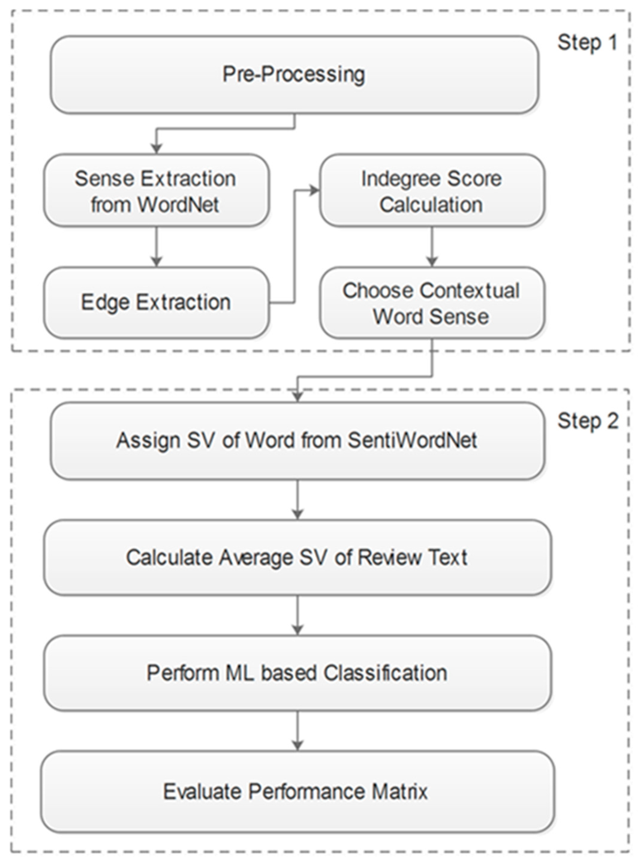
All steps carried out in this study are described in Figure 1. Step 1 was adopted from [13], which is an extension of [14]. This technique is called WSD. The aim of Step 1 was to assign a correct sentiment value to the words according to their contextual sense related to different neighboring words since the same words can appear in different parts of a text and may reveal different meanings, depending on the neighboring words. This problem is called polysemy. As shown in Figure 2, polysemy is a word with the same word form (WF) but a different meaning (WS). Some examples of polysemy can be seen in

Table 1. Example of polysemy.

Sentence	Sense	Sentiment Orientation
The girl runs to the school.	move fast on foot	Neutral
He runs the multinational company	direct or control	Positive
The land around here is flat.	having no variation in height	Neutral
The party is a bit flat.	uninteresting, boring	Negative
I enjoy the resolution of the screen.	get pleasure from	Positive
The company enjoys big profit.	have benefit from	Neutral

.

As shown in Table 1, the same sentiment word that appears in different review sentences potentially has a different sentiment orientation or value. This issue may interfere with the result of the SA. To address this problem, we employed a general purpose sentiment lexicon, namely SentiWordNet [4]. SentiWordNet specifies three sentiment values, namely positivity, negativity, and objectivity, to each synset of WordNet. More about SentiWordNet can be found at https://github.com/aesuli/sentiwordnet.

In the pre-processing step, stopword removal, stemming, part of speech (POS) tagging, and filtering were conducted. In the implementation, the Stanford POS tagger library was used. POS tagging is necessary to pick the correct sense of the words from the WordNet collection. In the filtering step, we left in only verbs, adjectives, and nouns. The local neighborhood used as the context for the words was a review sentence. Therefore, the processing step of WSD was done on a sentence basis.

After pre-processing (stop word removal, stemming, POS tagging, and filtering), the sense of the words from the WordNet collection was picked. As an example of the calculation of the proposed feature, consider the review sentence “I love the screen of the camera”. The result of the pre-processing step can be seen in

Table 2. Pre-processing step.

Step	Result
Picking Review Sentence	I love the screen of the camera.
POS tagging	I(PRP) - love(VBP) - the(DT) - screen(NN) - of(IN) - the(DT) - camera(NN)
Filtering	love(VBP) - screen(NN) – camera(NN)

.

After filtering, the left term is assigned to $w_i$. In the case of the example, we have $w_1,w_2$, and $w_3$. We then pick the senses of $w_i$ from the WordNet database, indicated as $w_i^j$, as shown in

Table 3. Senses and their notations.

Word	Notation	Senses from WordNet	Notation
love	$w_1$	have a great affection or liking for	$w{s}_1^1$
		get pleasure from	$w{s}_1^2$
		be enamored or in love with	$w{s}_1^3$
screen	$w_2$	a white or silvered surface where pictures can be projected for viewing	$w{s}_2^1$
		a protective covering that keeps things out or hinders sight	$w{s}_2^2$
camera	$w_3$	equipment for taking photographs (usually consisting of a lightproof box with a lens at one end and light-sensitive film at the other)	$w{s}_3^1$

.

In terms of the weighted graph, the senses of the words serve as the vertices of the graph. Adopting [25], the edges are then generated by calculating the similarity between the vertices using WordNet similarity measures from Wu and Palmer (WUP) [26], Leacock and Chodorow (LCH) [27], Resnik (RES) [28], Jiang and Conrath (JCN) [29], and Lin (LIN) [30]. Adapted Lesk [31] was incorporated to improve the result.

Suppose $e_{ab}^{cd}$ is the similarity between $w_a^b$ and $w_c^d$. All possible similarities between the word senses of the different words are calculated as shown in

Table 4. The calculation of all possible similarities between word senses of different words.

		$w_1$			$w_2$		$w_3$
		$w{s}_1^1$	$w{s}_1^2$	$w{s}_1^3$	$w{s}_2^1$	$w{s}_2^2$	$w{s}_3^1$
$w_1$	$w{s}_1^1$				$e_{12}^{11}$	$e_{12}^{12}$	$e_{13}^{11}$
	$w{s}_1^2$				$e_{12}^{21}$	$e_{12}^{22}$	$e_{13}^{21}$
	$w{s}_1^3$				$e_{12}^{31}$	$e_{12}^{32}$	$e_{13}^{31}$
$w_2$	$w{s}_2^1$						$e_{23}^{11}$
	$w{s}_2^2$						$e_{23}^{21}$
$w_3$	$w_3^1$

. For the implementation of WordNet similarity, the ws4j algorithm from Hideki Shima was adapted. The tool can be downloaded at https://ws4jdemo.appspot.com/. To select the contextual sense, the indegree score of each sense was computed using the indegree algorithm. For example, the indegree score of $w_1^3$ in Table 4, i.e., $In\left(w_1^3\right)$, is calculated as follows: $In\left(w_2^2\right)= e_{12}^{12}$ + $e_{12}^{22}$ + $e_{12}^{32}$ + $e_{23}^{21}$. In general, the indegree score of $w{s}_a^b$ is computed using Equation (1). The notation used in Equation (1) is described in

Table 5. Notations used in Equation (1).

Notations	Definitions
$In\left(w{s}_a^b\right)$	indegree score of $w{s}_a^b$
$e_{ka}^{lb}$	similarity value of word senses in the left side of $w{s}_a^b$
$o$	number of words in the left side of $w{s}_a^b$
$q_k$	number of word senses of word $w_k$
$e_{ab}^{mn}$	similarity value of word senses in the right side of $w{s}_a^b$
$p$	number of words in the right side of $w{s}_a^b$
$r_m$	number of word senses of word $w_m$

. In Table 4, the similarity highlights with red are the similarities between word senses on the left side of $w{s}_2^2$, and the similarity highlighted with green is the similarity of the word senses on the right side of $w{s}_2^2$. The indegree scores of all $w{s}_i^j$ are calculated, and the selected (contextual) sense is the sense of the word with the highest indegree score. The contextual sentiment value of a word, i.e., $c{s}_i$, is determined using Equation (2), where $f\left(m_i\right)$ assigns three sentiment values from SentiWordNet, called $cspo{s}_i$, $csne{g}_i$, and $csne{u}_i$. In Equation (3), $u$ is the number of words in the processed review sentence.

$$In\left(w{s}_a^b\right) = {\sum }_{k=1}^o{\sum }_{l=1}^{q_k}{e}_{ka}^{lb} + {\sum }_{m=1}^p{\sum }_{n=1}^{r_m}{e}_{am}^{bn}$$

(1)

$$c{s}_i = f\left(s_i\right),$$

(2)

where:

$$s_i = \underset{o}{\max } In{\left(w{s}_i^t\right)}_{t=1,2, \dots u}.$$

(3)

At the sentence level, three average sentiment values are calculated using Equations (4)–(6), respectively.

$$vpos = \frac{{\sum }_{i=1}^{u}cspo{s}_i}{u} ,$$

(4)

$$vneg = \frac{{\sum }_{i=1}^{u}csne{g}_i}{u},$$

(5)

$$vneu = \frac{{\sum }_{i=1}^{u}csne{u}_i}{u}$$

(6)

Regarding the utilized WordNet similarity algorithm, the average value of every contextual sense in the review document was then calculated and assigned as a feature of the review document. Three average sentiment scores from SentiWordNet were assigned to each document review. Hence, a set of 15 contextual features was provided as the basis for the classification task. A detailed description of the features is presented in

Table 6. Details of the proposed features.

Feature	Details
F1	Average positive score generated using WSD-WUP
F2	Average negative score generated using WSD-WUP
F3	Average neutral score generated using WSD-WUP
F4	Average positive score generated using WSD-LCH
F5	Average negative score generated using WSD-LCH
F6	Average neutral score generated using WSD-LCH
F7	Average positive score generated using WSD-RES
F8	Average negative score generated using WSD-RES
F9	Average neutral score generated using WSD-RES
F10	Average positive score generated using WSD-LIN
F11	Average negative score generated using WSD-LIN
F12	Average neutral score generated using WSD-LIN
F13	Average positive score generated using WSD-ADT
F14	Average negative score generated using WSD-ADT
F15	Average neutral score generated using WSD-ADT

.

For assessing the proposed features, an experiment was performed using five ML algorithms, namely Naïve Bayes, Logistic, Simple Logistic, Decision Tree, and Random Forest. We also applied five different feature selection methods, i.e., correlation-based feature selection (CFS), correlation attribute evaluator, information gain attribute evaluator, one rule attribute evaluator and principle component analysis, in order to test the performance of the proposed feature set in various different optimized combinations. For the implementation of the ML algorithms and the attribute selection methods, we used WEKA from the University of Waikato. The toolkit can be found at https://www.cs.waikato.ac.nz/ml/weka/. The employed attribute selection methods are briefly overviewed in the following paragraphs.

3.1. Correlation Feature Selection (CFS)

CFS argues that representative features are features that are highly correlated with the class, yet uncorrelated to each other. Therefore, it measures the individual predictive ability of each subset along with the degree of redundancy between them. CFS presents a measure called the ‘merit’ of the feature subsets. It predicts the correlation between a composite test consisting of the summed components and the outside variable using the standardized Pearson’s correlation coefficient [32], as shown in Equation (7).

$$r_{zc} =\frac{k\overline{r_{zi}}}{\sqrt{k+k\left(k-1\right)\overline{r_{ii}}}}$$

(7)

In Equation (7), $r_{zc}$ is defined as the correlation between the summed components and the outside variable, $k$ is the number of components, $\overline{r_{zi}}$ is the average of the correlation between the components and the outside variable, and $\overline{r_{ii}}$ is the average inter-correlation between the components.

3.2. Correlation Attribute Evaluator

This method calculates the weighted average of the overall Pearson correlation coefficient between an attribute and its class as an indicator for ranking a set of attributes. For $x\in X$ and $c\in C$, where $X$ is the feature subset and $C$ is the class, and Pearson’s correlation coefficient is given by Equation (8).

$$r = \frac{{\sum }_{i=1}^n\left(x_i-\overline{x}\right)\left(c_i-\overline{c}\right)}{\sqrt{{\sum }_{i=1}^n{\left(x_i-\overline{x}\right)}^2}\sqrt{{\sum }_{i=1}^n{\left(c_i-\overline{c}\right)}^2}} .$$

(8)

3.3. Information Gain Attribute Evaluator

Information gain, also called mutual information, can also reveal dependency between features by calculating the level of impurity in a group of samples. This technique provides a ranking of attributes by evaluating the information gain of an attribute with respect to the class. The information gain of $X$ for $C$ is the class, and $X$ is the attribute subset given by Equation (9).

$$IG(C|X) = H\left(C\right)-H(C|X).$$

(9)

3.4. OneR Attribute Evaluator

The one rule attribute evaluator rates the values of the attributes based on a simple yet accurate classifier called the one rule classifier [33], which classifies a dataset based on a single attribute, i.e., a one-level decision tree. OneR chooses the rule with the smallest error rate from previously built rules for every attribute in the training data.

3.5. Principle Components

The algorithm attempts to find the axis of greatest variance of the data. In the implementation, this attribute evaluator calculates the eigenvector of the covariance matrix of the data and filters out the attributes with the worst eigenvectors.

4. Result and Discussion

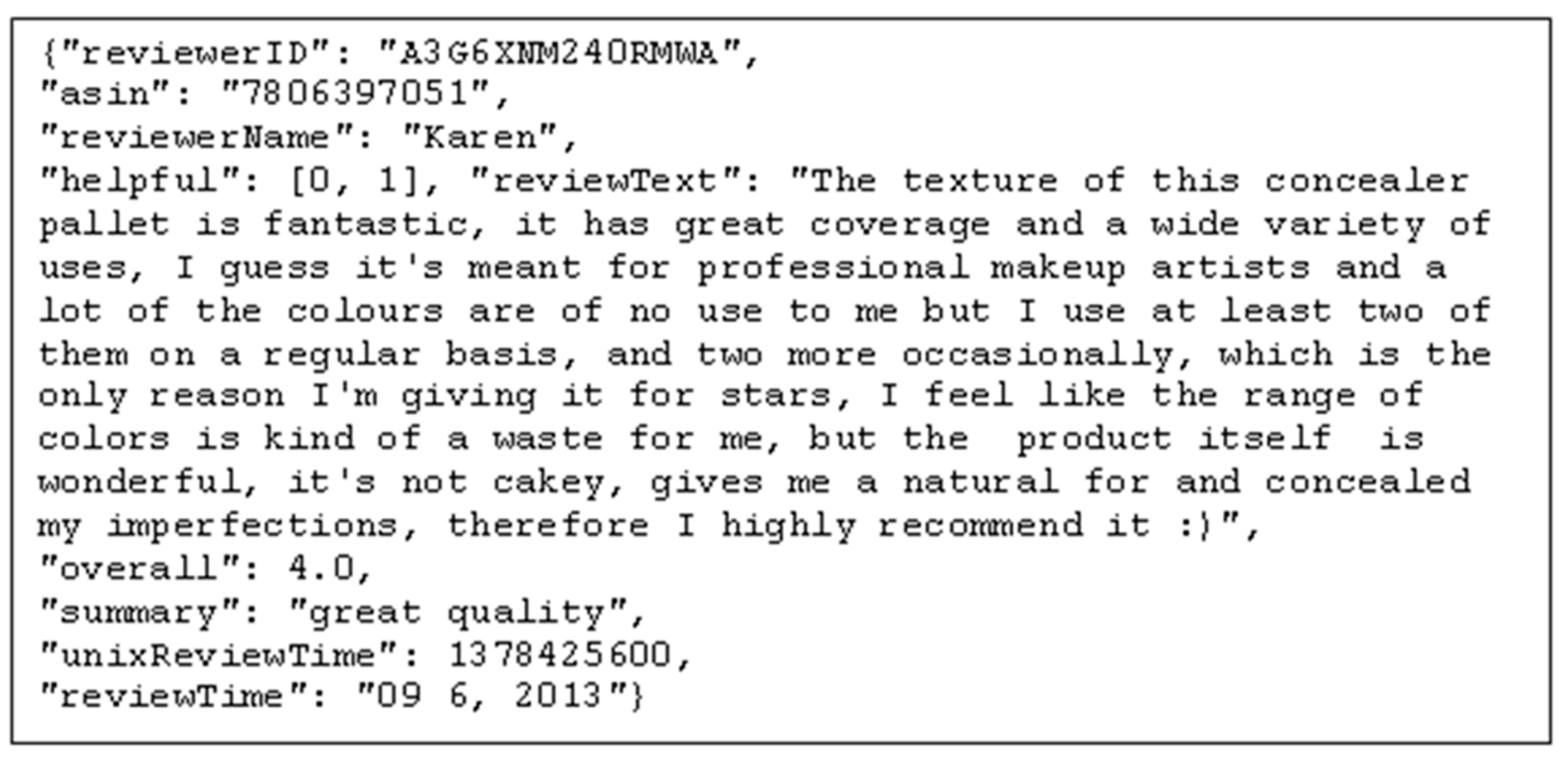
In the experiment, we used three product review datasets from Amazon Review Data provided by Julian McAuley [23], i.e., Beauty, Books, and Movies. The dataset can be downloaded from http://jmcauley.ucsd.edu/data/amazon/. For building the ground truth, we assigned a label of three sentiment categories, i.e., positive, negative, and neutral, for every product review document by taking the ‘overall’ score from the metadata of the dataset (see the sample review in Figure 3.). The datasets with an ‘overall’ score of 1–2 were labeled as negative reviews. Meanwhile, the datasets with an ‘overall’ score of 4–5 were labeled as positive. The rest was labeled as neutral.

We present the results of the experiment using the three Jean McAuley Amazon datasets in

Table 7. Result of experiment using Beauty dataset. FS = Feature Selection; CFS = Correlation Feature Selection; IG = Information Gain; PCA = Principal Component Analysis; Prec = precision; Rec = recall; Fmeas = F-Measure.

FS Method	Algor	Baseline 1			Baseline 2			Proposed Method
		Prec	Rec	Fmeas	Prec	Rec	Fmeas	Prec	Rec	Fmeas
None	NB	0.768	0.735	0.750	0.737	0.708	0.722	0.817	0.648	0.714
	NBM	0.853	0.853	0.853	0.708	0.708	0.708	0.800	0.855	0.827
	LOG	0.725	0.833	0.775	0.709	0.823	0.762	0.801	0.869	0.834
	SLOG	0.853	0.853	0.853	0.706	0.802	0.751	0.804	0.897	0.848
	DT	0.726	0.843	0.780	0.708	0.813	0.756	0.823	0.869	0.843
	RF	0.807	0.853	0.802	0.769	0.833	0.784	0.847	0.883	0.860
CFS	NB	0.853	0.853	0.853	0.737	0.708	0.722	0.803	0.890	0.844
	NBM	0.768	0.735	0.750	0.736	0.750	0.743	*0.897	*1.000	*0.945
	LOG	0.725	0.833	0.775	0.709	0.823	0.762	*0.897	*1.000	*0.945
	SLOG	0.768	0.735	0.750	0.706	0.802	0.751	0.803	0.890	0.844
	DT	0.853	0.853	0.853	0.708	0.813	0.756	0.803	0.890	0.844
	RF	0.813	0.853	0.815	0.750	0.750	0.750	0.802	0.876	0.837
CORELL	NB	0.768	0.735	0.750	0.737	0.708	0.722	0.815	0.634	0.704
	NBM	0.853	0.853	0.853	0.736	0.750	0.743	0.800	0.862	0.830
	LOG	0.725	0.833	0.775	0.709	0.823	0.762	0.804	0.897	0.848
	SLOG	0.853	0.853	0.853	0.786	0.833	0.797	0.804	0.897	0.848
	DT	0.726	0.843	0.780	0.711	0.833	0.767	0.803	0.890	0.844
	RF	0.807	0.853	0.802	0.769	0.833	0.784	0.800	0.862	0.830
IG	NB	0.768	0.735	0.750	0.737	0.708	0.722	0.809	0.821	0.815
	NBM	0.853	0.853	0.853	0.708	0.708	0.708	0.804	0.897	0.848
	LOG	0.723	0.833	0.775	0.709	0.823	0.762	0.801	0.869	0.834
	SLOG	0.768	0.735	0.750	0.706	0.802	0.751	0.804	0.897	0.848
	DT	0.726	0.843	0.780	0.708	0.813	0.756	0.804	0.897	0.848
	RF	0.807	0.853	0.802	0.769	0.833	0.784	0.802	0.876	0.837
OneR	NB	0.768	0.735	0.750	0.737	0.708	0.722	0.804	0.676	0.730
	NBM	0.853	0.853	0.853	0.736	0.750	0.743	0.804	0.897	0.848
	LOG	0.725	0.833	0.775	0.709	0.823	0.762	0.801	0.869	0.834
	SLOG	0.768	0.735	0.750	0.706	0.802	0.751	0.804	0.897	0.848
	DT	0.726	0.843	0.780	0.708	0.813	0.756	0.803	0.883	0.841
	RF	0.807	0.853	0.802	0.769	0.833	0.784	0.855	0.890	0.864
PCA	NB	0.726	0.843	0.780	0.708	0.813	0.756	0.818	0.855	0.835
	NBM	0.726	0.843	0.780	0.745	0.813	0.771	0.804	0.897	0.848
	LOG	0.725	0.833	0.775	0.711	0.833	0.767	0.801	0.869	0.834
	SLOG	0.781	0.843	0.796	0.754	0.823	0.777	0.804	0.897	0.848
	DT	0.725	0.833	0.775	0.711	0.833	0.767	0.803	0.890	0.844
	RF	0.781	0.843	0.796	0.709	0.823	0.762	0.828	0.876	0.847

,

Table 8. Result of experiment using Books dataset.

FS Method	Algor	Baseline 1			Baseline 2			Proposed Method
		Prec	Rec	Fmeas	Prec	Rec	Fmeas	Prec	Rec	Fmeas
None	NB	0.663	0.701	0.679	0.722	0.762	0.741	0.824	0.824	0.824
	NBM	0.737	0.770	0.746	0.722	0.762	0.741	0.829	0.882	0.855
	LOG	0.707	0.747	0.720	0.706	0.667	0.686	0.882	0.882	0.882
	SLOG	0.707	0.770	0.714	0.729	0.810	0.767	0.829	0.882	0.855
	DT	0.607	0.759	0.674	0.706	0.667	0.686	0.826	0.853	0.839
	RF	0.601	0.724	0.657	0.729	0.810	0.767	0.829	0.882	0.855
CFS	NB	0.678	0.747	0.699	0.779	0.714	0.742	0.826	0.853	0.839
	NBM	0.678	0.747	0.699	0.714	0.714	0.714	0.826	0.853	0.839
	LOG	0.707	0.770	0.714	0.722	0.762	0.741	0.829	0.882	0.855
	SLOG	0.707	0.770	0.714	0.722	0.762	0.741	0.821	0.794	0.807
	DT	0.607	0.759	0.674	0.714	0.714	0.714	0.821	0.794	0.807
	RF	0.668	0.736	0.692	0.706	0.667	0.686	0.826	0.853	0.839
CORELL	NB	0.663	0.701	0.679	0.722	0.762	0.741	0.824	0.824	0.824
	NBM	0.737	0.770	0.746	0.729	0.810	0.767	0.829	0.882	0.855
	LOG	0.707	0.747	0.720	0.706	0.667	0.686	0.882	0.882	0.882
	SLOG	0.707	0.770	0.714	0.729	0.810	0.767	0.829	0.882	0.855
	DT	0.607	0.759	0.674	0.714	0.714	0.714	0.821	0.794	0.807
	RF	0.601	0.724	0.657	0.729	0.810	0.767	0.817	0.765	0.790
IG	NB	0.663	0.701	0.679	0.722	0.762	0.741	0.824	0.824	0.824
	NBM	0.737	0.770	0.746	0.722	0.762	0.741	0.829	0.882	0.855
	LOG	0.707	0.747	0.720	0.706	0.667	0.686	0.882	0.882	0.882
	SLOG	0.707	0.770	0.714	0.714	0.714	0.714	0.826	0.853	0.839
	DT	0.607	0.759	0.674	0.706	0.667	0.686	0.824	0.824	0.824
	RF	0.601	0.724	0.657	0.729	0.810	0.767	0.817	0.765	0.790
OneR	NB	0.663	0.701	0.679	0.722	0.762	0.741	0.824	0.824	0.824
	NBM	0.737	0.770	0.746	0.722	0.762	0.741	0.829	0.882	0.855
	LOG	0.707	0.747	0.720	0.706	0.667	0.686	0.882	0.882	0.882
	SLOG	0.707	0.770	0.714	0.714	0.714	0.714	0.826	0.853	0.839
	DT	0.607	0.759	0.674	0.706	0.667	0.686	0.826	0.853	0.839
	RF	0.601	0.724	0.657	0.729	0.810	0.767	0.829	0.882	0.855
PCA	NB	0.710	0.736	0.720	0.722	0.762	0.741	0.829	0.882	0.855
	NBM	0.710	0.736	0.720	0.706	0.667	0.686	0.826	0.853	0.839
	LOG	0.749	0.782	0.754	0.722	0.762	0.741	*0.916	*0.882	*0.895
	SLOG	0.769	0.793	0.729	0.792	0.762	0.776	0.826	0.853	0.839
	DT	0.678	0.747	0.699	0.714	0.714	0.714	0.829	0.882	0.855
	RF	0.705	0.759	0.718	0.729	0.810	0.767	0.824	0.824	0.824

and

Table 9. Result of experiment using Movies Dataset.

FS Method	Algor	Baseline 1			Baseline 2			Proposed Method
		Prec	Rec	Fmeas	Prec	Rec	Fmeas	Prec	Rec	Fmeas
None	NB	0.649	0.682	0.664	0.691	0.738	0.708	0.691	0.710	0.700
	NBM	0.739	0.765	0.748	0.743	0.774	0.752	0.746	0.770	0.756
	LOG	0.670	0.718	0.688	0.659	0.714	0.682	0.695	0.750	0.718
	SLOG	0.671	0.741	0.692	0.613	0.762	0.680	0.723	0.800	0.736
	DT	0.660	0.753	0.685	0.683	0.726	0.700	0.723	0.750	0.735
	RF	0.629	0.718	0.664	0.672	0.762	0.698	0.706	0.790	0.730
CFS	NB	0.765	0.788	0.723	0.730	0.786	0.712	0.887	0.920	0.903
	NBM	0.765	0.788	0.723	0.743	0.774	0.752	*0.943	*1.000	*0.970
	LOG	0.720	0.766	0.699	0.615	0.774	0.686	0.888	0.937	0.912
	SLOG	0.720	0.766	0.699	0.615	0.774	0.686	0.943	1.000	0.970
	DT	0.660	0.753	0.685	0.613	0.762	0.680	0.943	1.000	0.970
	RF	0.671	0.741	0.692	0.607	0.726	0.661	0.888	0.931	0.909
CORELL	NB	0.649	0.682	0.664	0.691	0.738	0.708	0.681	0.720	0.699
	NBM	0.739	0.765	0.748	0.743	0.774	0.752	0.695	0.750	0.715
	LOG	0.670	0.718	0.688	0.659	0.714	0.682	0.701	0.760	0.724
	SLOG	0.671	0.741	0.692	0.613	0.762	0.680	0.723	0.800	0.736
	DT	0.660	0.753	0.685	0.683	0.726	0.700	0.695	0.750	0.715
	RF	0.629	0.718	0.664	0.672	0.762	0.698	0.753	0.780	0.763
IG	NB	0.649	0.682	0.664	0.691	0.738	0.708	0.753	0.677	0.710
	NBM	0.739	0.765	0.748	0.743	0.774	0.752	0.680	0.760	0.713
	LOG	0.670	0.718	0.688	0.659	0.714	0.682	0.687	0.770	0.719
	SLOG	0.671	0.741	0.692	0.613	0.762	0.680	0.706	0.790	0.730
	DT	0.660	0.753	0.685	0.683	0.726	0.700	0.675	0.750	0.707
	RF	0.629	0.718	0.664	0.672	0.762	0.698	0.716	0.780	0.737
OneR	NB	0.649	0.682	0.664	0.691	0.738	0.708	0.710	0.750	0.727
	NBM	0.739	0.765	0.748	0.743	0.774	0.752	0.695	0.780	0.725
	LOG	0.670	0.718	0.688	0.659	0.714	0.682	0.695	0.780	0.725
	SLOG	0.671	0.741	0.692	0.613	0.762	0.680	0.756	0.810	0.724
	DT	0.660	0.753	0.685	0.683	0.726	0.700	0.650	0.770	0.705
	RF	0.629	0.718	0.664	0.672	0.762	0.698	0.708	0.770	0.730
PCA	NB	0.691	0.729	0.706	0.733	0.762	0.743	0.723	0.750	0.735
	NBM	0.691	0.729	0.706	0.634	0.619	0.626	0.810	0.810	0.810
	LOG	0.678	0.729	0.696	0.691	0.738	0.708	0.708	0.770	0.730
	SLOG	0.599	0.753	0.667	0.773	0.798	0.736	0.727	0.795	0.820
	DT	0.601	0.765	0.673	0.650	0.738	0.684	0.643	0.730	0.684
	RF	0.713	0.765	0.720	0.696	0.762	0.712	0.884	0.874	0.879

. Our proposed features were evaluated using Naïve Bayes, Naïve Bayes, Logistic, Simple Logistic, J48, and Random Forest. The combination of features was optimized using CFS, correlation attribute evaluator, information gain attribute evaluator, one-rule attribute evaluator, and principle component analysis, and then we compared the results with the full feature set. The performance metrics of the selected features were evaluated using 10-fold cross-validation.

To investigate the role of semantic features in enhancing the result of the supervised SA method, the performance of our proposed features was compared with a baseline feature. For the baseline, we applied Unigram features, i.e., common features used for text classification, extracted using an unsupervised filter from StringtoWordVector in WEKA. In the experiment, we also applied the same feature selection method for the baseline. For the performance metrics, precision, recall, and F-Measure were employed. The whole experiment was conducted using 10-fold cross-validation with WEKA. The results of the experiment are presented in Table 7, Table 8 and Table 9. We compared the result of experiment with two baseline methods, i.e., Unigram (Baseline 1) and Bigram (Baseline 2), of BoW that are commonly adopted for supervised SA tasks.

In Table 7, Table 8 and Table 9, we provide the experiment results for the three product review datasets, i.e., Beauty, Books, and Movies dataset. In each table, we compare the performance of the proposed features with two baselines, namely Unigram and Bigram, that are commonly employed for text classification tasks. The results are grouped based on the employed feature selection method. For every feature selection method, we applied all used ML algorithms. To indicate the best performance achieved for precision, recall, and F-Measure, we used the asterisk symbol as presented in the Tables. For the Beauty dataset, the best performance of the proposed features is 0.897, 1.000, and 0.945 for precision, recall, and F-Measure, respectively. For the Books dataset, Principal Component Analysis (PCA) achieved the best performance by 0.916, 0.882, and 0.895 for precision, recall, and F-Measure, respectively. Meanwhile, for the Movies dataset, features selected using CFS reached the best performance by 0.943, 1.000, and 0.970 for precision, recall, and F-Measure, respectively.

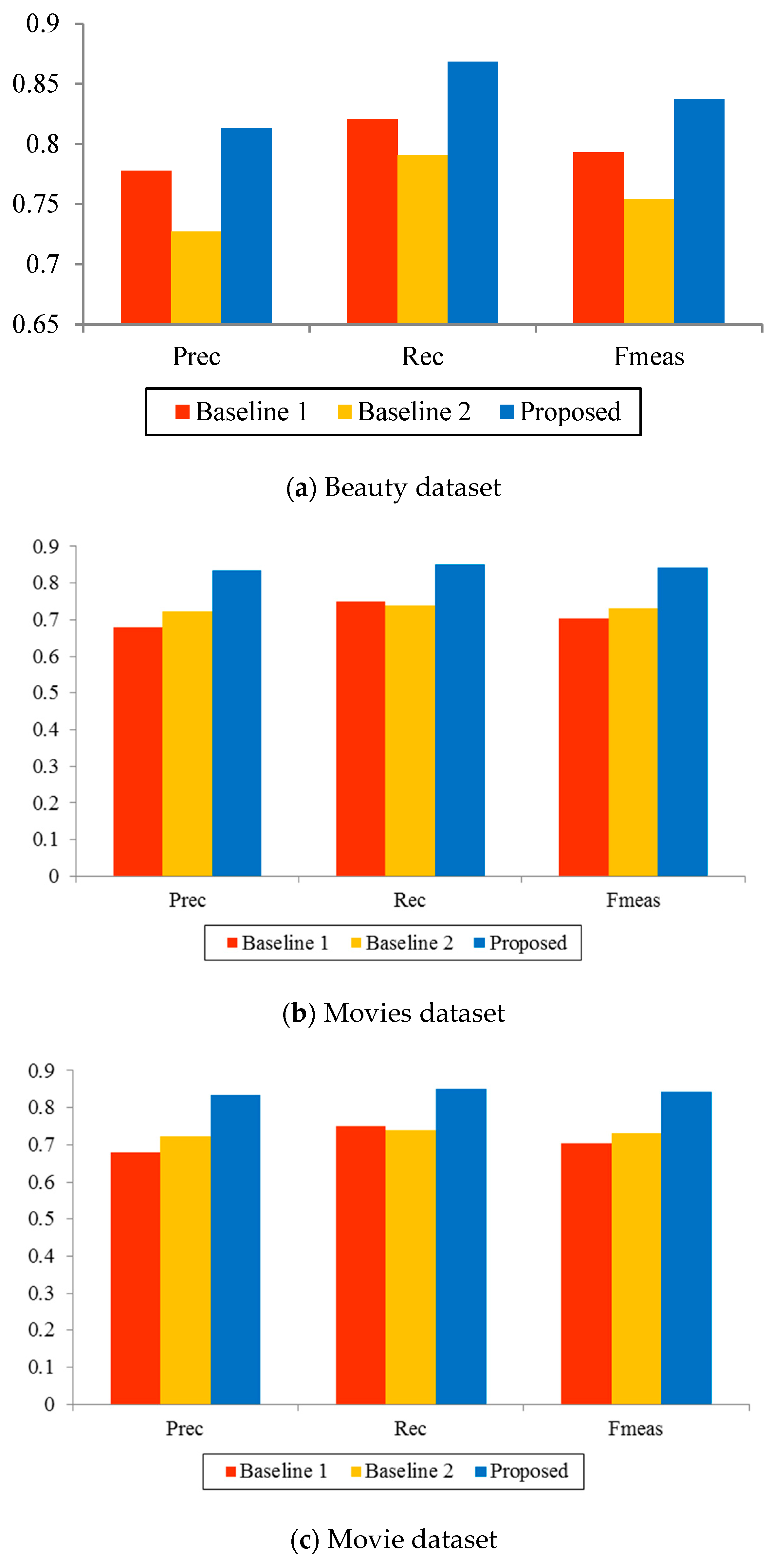
In Figure 4, we calculated the average performance of our proposed features in terms of precision, recall, and F-Measure. Compared with the baseline feature that is commonly employed in the supervised SA task, i.e., BOW, the extracted semantics features have favorably increased all performance metrics of the supervised SA task, i.e., precision, recall, and F-Measure, as indicated in Figure 4. In the figure, we present average evaluation metrics for the three datasets. The figure indicates that the proposed semantic features outperform both Unigram and Bigram in all performance metrics. On average, the proposed features increased precision, recall, and F-Measure by 10.9%, 9.2%, and 10.6% of those compared to baseline methods.

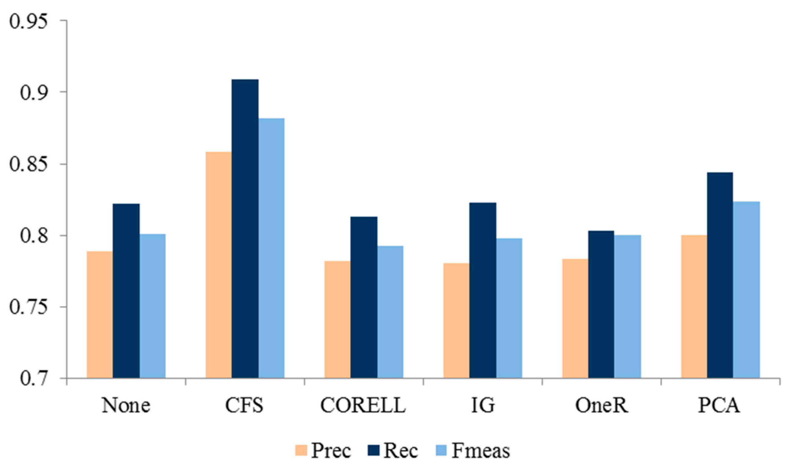
To find the best set of the features, we calculated the average performance of our semantic features for every feature selection method, as presented in Figure 5. The results of the experiment presented in Figure 5 confirmed that the best semantic feature set is one that is selected using CFS, i.e., F1–6. Features selected using PCA are in second place. We also highlight that the employed WordNet similarity algorithms have a dominant role in determining the correct sentiment value of a term. Assigning incorrect sentiment values results in extracting contextual features that potentially lead to misclassification.

The limitation of this study is that the performance of the adopted similarity algorithm is not what was expected. As an example, we calculate semantic similarity of love#v#1, hate#v#1, and like#v#1 using $wup,jcn,$ and $lch$. Naturally, we expected that love#v#1 and like#v#1 should have greater semantic similarity than love#v#1 and hate#v#1. Sense of those words can be seen in

Table 10. Sense picked from WordNet.

Term	Sense Picked from WordNet Database
love#v#1	have a great affection or liking for
hate#v#1	dislike intensely
like#v#1	Prefer or wish to do something

. Yet, the result was not what we wished, as indicated in

Table 11. Result of semantic similarity.

WordNet Similarity Algorithm	Semantic Similarity of
	Love#v#1 and Hate#v#1	Love#v#1 and Like#v#1
wup	0.04	0.04
jcn	0.06	0.07
lch	1.95	1.94

. In the future, we plan to propose a robust similarity algorithm to augment the result of a supervised SA task.

Implications

The implications comprise practical implication for both online marketers and customers, as well as academic implications for the researcher in the field of text processing. The results of study affirm that our proposed SA technique can be employed to generate quantitative ratings from unstructured text data within the product review [34]. The online marketers could, therefore, apply the technique to foresee consumer satisfaction toward a certain product [35]. Meanwhile, for potential customers, a big data recommender system could possibly be built accordingly to provide recommendation about the intended product they want to purchase [2]. The finding of this work could also be beneficial for researchers in the field of text processing to further explore more sophisticated semantic features of words. Previous work has also confirmed the robustness of semantic features [10].

5. Conclusions

This paper proposed a set of contextual features for SA of product reviews, generated using an extended WSD method. Several ML algorithms were employed to evaluate the performance of the proposed features in a supervised SA task. To find the subset that provides the best performance metrics, several feature selection methods were applied, i.e., CFS, correlation attribute evaluator, information gain attribute evaluator, one-rule attribute evaluator, and principle component analysis.

This study contributes to improving the performance of supervised SA tasks by proposing a method to extract semantic features of the product review dataset. The results of the cross-validated experiment in a supervised environment using several ML algorithms and feature selection methods has confirmed that our proposed semantic features favorably augment the performance of SA in terms of precision, recall, and F-Measure. Another finding of this study summarizes the robustness of semantic feature set selected using CFS and PCA.