An Efficient Multicore Algorithm for Minimal Length Addition Chains

Abstract

A minimal length addition chain for a positive integer m is a finite sequence of positive integers such that (1) the first and last elements in the sequence are 1 and m, respectively, (2) any element greater than 1 in the sequence is the addition of two earlier elements (not necessarily distinct), and (3) the length of the sequence is minimal. Generating the minimal length addition chain for m is challenging due to the running time, which increases with the size of m and particularly with the number of 1s in the binary representation of m. In this paper, we introduce a new parallel algorithm to find the minimal length addition chain for m. The experimental studies on multicore systems show that the running time of the proposed algorithm is faster than the sequential algorithm. Moreover, the maximum speedup obtained by the proposed algorithm is 2.5 times the best known sequential algorithm.

1. Introduction

Given a positive integer m, an addition chain (AC) for m is a finite sequence of positive integers such that the first and last elements in the sequence are 1 and m, respectively, while any other element greater than 1 comes from the addition of two earlier elements (not necessarily distinct). Mathematically, we can write the elements of the sequence of length l as follows [1].

$$\begin{gathered} s_0=1,\hspace{1em}{s}_l=m \\ {s}_k=s_i+s_j, 1\le k\le l\mathrm{and}0\le i\le j<k. \end{gathered}$$

The importance of generating such chains comes from the equivalence between generating a minimal length AC for m and reducing the number of multiplications to compute the modular exponentiation, X^m mod N, where the modular exponentiation is a fundamental operation in asymmetric cryptosystems [2,3,4]. If we find a minimal length chain for the positive integer m, then we can compute X^m by a minimal number of multiplications.

There are some notations and definitions related to ACs, which are [5,6]:

• $\lambda \left(m\right)=\lfloor {log}_{2}m\rfloor$, where $\lambda$ is the length in bits for the given number m [5].
• Given m as a binary representation, v(m) is the number of 1s in m.
• The $k^{th}$ step in the chain is called $\{\begin{array}{cc}doubling& if i=j=k-1\hfill \\ star& if i=k-1\hfill \\ small& if \lambda \left(s_k\right)=\lambda \left(s_{k-1}\right)\hfill \\ big& if \lambda \left(s_k\right)=\lambda \left(s_{k-1}\right)+1\hfill \end{array}$
• The number of small steps in the chain up to s_k is denoted by S(s₀, s₁, …, s_k) and the number of big steps is $\lambda \left(s_k\right)$.
• The length of AC, l, for m can be written in terms of the number of small steps and $\lambda \left(m\right)$ as follows.

  $$l=\lambda \left(m\right)+S\left(s_0, s_1, \dots , s_k=m\right)$$
• If l is minimal then the chain is called the minimal length addition chain (MLAC) or the shortest addition chain and the length of the chain is denoted by $\ell \left(m\right).$ Otherwise, the chain is called a short addition chain (SAC).

The following two sequences represent a short and minimal length AC for the number 25. The first chain is (1, 2, 4, 6, 10, 16, 22, 24, 25) of length eight, while the second chain is (1, 2, 3, 5, 10, 20, 25) of length six.

Algorithms for generating ACs [5,6,7,8,9,10,11,12,13,14,15] can be classified into two main types. The first type is the exact algorithm, which generates the MLAC, while the second type is an approximation algorithm, which generates an SAC. The main benefit of the first type of algorithm is that the length of the generated chain is minimal. However, the running time of these algorithms increases rapidly with the increasing size of m and more importantly with the increasing size of v(m). For the second type of algorithm, the main benefit is that the running time is small. However, the length of the chain is not generally the shortest. In this work, we will focus mainly on the first type of algorithm.

For the MLAC, many different algorithms have been introduced based on many strategies, such as graph, depth-first search (DF), and branch and bound (B&B) [5,6,10,15,16]. Bleichenbacher and Flammenkamp [16] described a method based on a directed acyclic graph to find an MLAC up to a certain positive integer m. Clift [10] used the same strategy to present a fast algorithm that is used to compute the ranges of optimal ACs. Otherwise, the algorithm is slow. The DF search is based on traversing the search space (tree) starting from the first element of the chain, s₀ = 1, and exploring every branch as far as possible before backtracking. The method was used by Chin and Tsai [17] to generate the MLAC. This method is improved by introducing some bounding and pruning methods to delete the branches of the search space. The method is called the B&B strategy. Thurber [15] introduced three bounding sequences and two pruning methods to reduce the time of searching for MLACs. Bahig [5] introduced modifications for Thurber’s algorithm to improve the running time for an MLAC. The modifications include new sufficient conditions and lower bounds for star and non-star steps, respectively. Additionally, Bahig [6] proposed a star reductions strategy that improves the running time and storage for finding MLACs by 38–58% and 26–45%, respectively.

In order to accelerate the computational time to generate an MLAC, we will use high-performance computing concepts for this goal. Different modern high-performance systems are introduced, such as multicores, Graphics Processing Units (GPUs), and Field-Programmable Gate Arrays (FPGAs). A small number of research papers [7,18] are introduced to solve the AC problem from the view of parallelism. The results in these papers were theoretical studies without any implementation. Moreover, the papers are concerned with how to find short, not the shortest, chains. In this paper, we are interested in finding the MLAC using parallelism since the running time for an MLAC is large.

The main contribution of this work is designing a new parallel algorithm for finding an MLAC. The introduced algorithm uses two different strategies for searching: DF and breadth-first (BF). Then, we evaluate and measure the performance of it by implementing the proposed algorithm using the OpenMP library with the C++ language on a multicore system of 12 cores. The experimental studies show that the running time of the proposed algorithm is faster than the sequential algorithm with a maximum speedup of 2.5. Additionally, the proposed parallel algorithm is different than the two previous parallel algorithms [7,18] in many respects. First, the main objective of the works in [7,18] is to find a short AC (not necessary minimal length), while the main objective of our work is to design the shortest AC (necessary minimal length). Second, the running time for the two algorithms in [7,18] is polynomial time because the solution is an approximation. The running time for the proposed algorithm is exponential because the solution is exact. Third, the two algorithms in [7,18] are based on a binary method (right–left or left–right), while the proposed parallel algorithm is based a hybrid strategy that consists of DF and BF.

The paper is organized as an introduction, three sections, and a conclusion. In the second section, we describe briefly the best known sequential algorithm to generate an MLAC for the positive integer m. Section 3 contains the main idea and steps of the proposed parallel algorithm. The experimental study of the introduced algorithm is presented in Section 4. In this section, we studied the behavior of the proposed algorithm according to running time, storage, and speedup. Finally, we conclude our work in Section 5.

2. The Best Known Sequential AC Algorithm

In this section, we briefly describe the best known sequential algorithm to find an AC with minimal length. The algorithm is based on the B&B strategy and consists of the following steps [5,6].

Step 1:

Compute the lower bound of l(m), say Lb.

Step 2:

Loop the following:

2.1:

Compute the bounding sequences, Bs.

2.2:

Initialize the two stacks T₁ and T₂ by pushing the elements s₀ = 1 and s₁ = 2 on T₁ and the levels 0 and 1 on T₂. Also, initialize the current level with 1, k = 1.

2.3:

Repeat

• Push on T₁ all possible elements (star and non-star) s_k+1, after applying pruning conditions for s_k.
• Push on T₂ the levels, k + 1, of all elements pushed in the previous step.
• Pop the stack T₂ and assign the top to k.
• Pop the stack T₁ and assign it to the current element s_k.
• If the current element s_k equals the goal m then return the minimal length chain s₀ s₁ …s_k.
  Until k < 2.

2.4:

Increase the lower bound by 1, Lb = Lb + 1.

The lower bound for l(m) can be computed by using the previous results that were introduced by Thurber [15] and Schönhage [19]. If v(m) $\le 16$, then the lower bound equals to $\lambda \left(m\right)+\lceil {log}_{2}v(m)\rceil$; otherwise, the lower bound equals to the ceiling value of the term ${log}_{2}m+{log}_{2}v(m)-2.13$.

To compute the bounding sequences, we can write any positive integer number, m, as m = 2^q d, q ≥ 0, and d is odd. Then, Thurber [15] introduced three bounding sequences as follows:

$$bs{1}_k=\lceil \frac{m 2^k}{2^{Lb}}\rceil , 0\le k\le Lb$$

$$bs{2}_k=\{\begin{array}{cc}\lceil \frac{m 2^{k+2}}{3 2^{Lb}}\rceil & 0\le k\le Lb-q-2\\ \lceil \frac{m 2^k}{2^{Lb}}\rceil & Lb-q-1\le k\le Lb\end{array}$$

$$bs{3}_k=\{\begin{array}{cc}\lceil \frac{m }{2^q \left(2^{Lb-q-k-1}+1\right)}\rceil & 0\le k\le Lb-q-2\\ \lceil \frac{m 2^k}{2^{Lb}}\rceil & Lb-q-1\le k\le Lb\end{array}$$

Thurber [15] suggested two types of pruning using these bounding sequences. The first one is called vertical (Vbs), and is used when $s_k<bs{1}_k$ (or $bs{2}_k, bs{3}_k$). The second one is called slant (Sbs), and is used when $s_k+s_{k-1}<bs{1}_{k+1}$ (or $bs{2}_{k+1}$). The conditions for using these types of pruning are as follows.

• For vertical bounds, if $m= \left(2^i+1\right) j$ for some $i>0$ apply $bs{2}_k$ for Vbs, while if $m\ne \left(2^i+1\right) j$ for any $i>0$ apply $bs{3}_k$ for Vbs.
• For slant bounds, if $m\ne 5 i$ then apply $bs{2}_k$ for Sbs, while if $m=5 i$ then apply $bs{1}_k$ for Sbs.

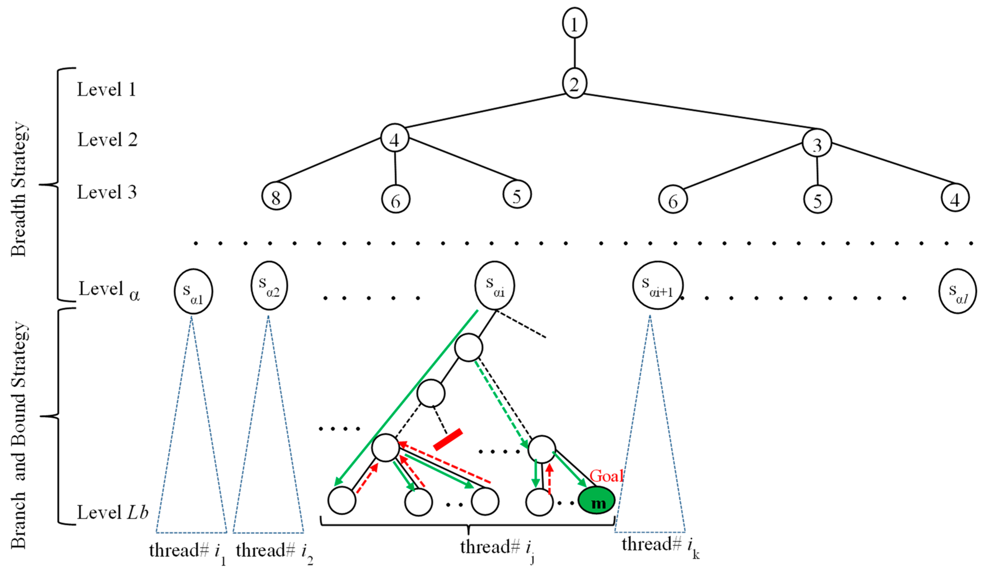
3. Methodology

In this section, we present the proposed algorithm to find an AC with minimal length using the parallel strategies. The section consists of two subsections. The first subsection includes the main stages of the parallel proposed algorithm, while the details for the stages are introduced in the second subsection.

3.1. Main Stages

The main idea to design a parallel algorithm for an AC is based on traversing the search space in two stages. The first stage traverses the search space by using the BF strategy to level α in a sequential way. The second stage traverses the search space by using the DF strategy in a parallel way. In both stages, we used all previous bounding sequences and conditions to prune the search tree.

For the first stage, each path from the root to a leaf in the tree of the α level represents a list ($s_{\alpha }, s_{\alpha -1},\dots ,s_1=2,s_0=1$). Each path to a leaf in the tree is a potential partial chain to m. All paths generated from this stage are stored in a queue Q. For the second stage, the multicore system takes each member of the queue and processes it to try to find an addition chain to m of Lb length. With ($s_{\alpha }, s_{\alpha -1},\dots ,s_1=2,s_0=1$), all candidates for an addition chain start with $s_0=1$, $s_1=2$, …, $s_{\alpha -1}$, $s_{\alpha }$ and so forth. If the multicore system has c cores, then c elements are taken off the queue and processed in parallel. The first Q element to generate an addition chain for m stops the process. If no addition chain of length Lb is found and the number of elements in the queue, |Q|, exceeds c, then more elements from the queue are loaded to process. If all the elements from the queue have been exhausted and no addition chain of length Lb is found, then Lb is incremented by one and the process is repeated. It is noted that if |Q| > c then queue elements are taken off the queue in chunks, in which case the search is part parallel and part sequential (see Figure 1).

The proposed algorithm consists of six steps as follows.

Step 1:

Compute the lower bound of l(m), say Lb.

Step 2:

Compute the vertical and slant bounding sequences.

Step 3:

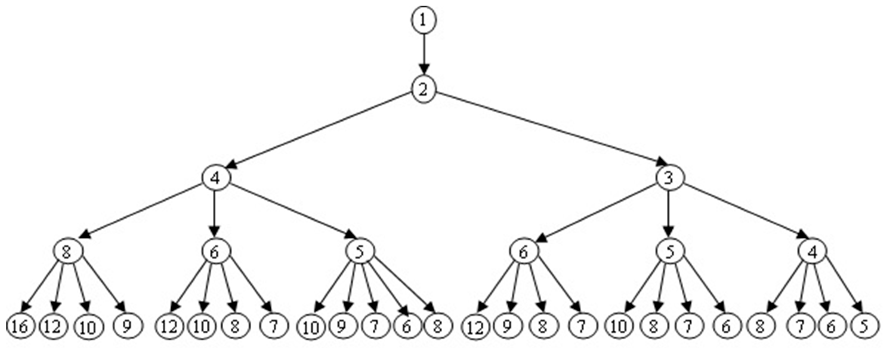
Generate the breadth tree until level α and assign it to a queue Q.

Step 4:

Each core will assign one element e from the queue Q, and then we use the best known B&B algorithm to find the goal m.

Step 5:

If one core finds the goal then terminate the process of searching. Otherwise, repeat Step 4 on a new element from the queue if not empty.

Step 6:

If the queue is empty then increase the lower bound by one and repeat Steps 2–5.

The first three steps will be executed sequentially, while the fourth and fifth steps will be executed concurrently. The last step will be executed sequentially. Additionally, the main aim of Step 1 is to start the search of the goal m with the lower bound Lb, while the aim of Step 2 is determining the bounding sequences that are used to delete some elements in the level that cannot lead to the goal m with length Lb. The aim of Step 3 is to construct the different partial chains with length α. The aim of Steps 4 and 5 is to complete the construction of addition chains concurrently. The main purpose of Step 6 is to increment Lb by 1 and repeat the search.

The first step will be executed only one time at the start of the algorithm, while Steps 2 and 3 will be executed with every new lower bound. The number of executions for Steps 4 and 5 depend on three factors: (1) the number of elements in the queue; (2) the number of cores; and (3) the existence of the goal with length Lb. The number of elements in the queue depends on the value of α that will be determined in the next subsection.

3.2. Implementation Details

In this subsection, we will give some details about each step of the proposed parallel algorithm.

For Step 1 and 2, the details exist in Section 2 without any change. For Step 3, no theoretical studies, to date, exist to determine what is the best value for the value α, because the behavior of the problem, MLAC, is difficult. We will discuss later in the experimental study that the value of α depends on the memory of the machine.

Now, we will discuss how to construct the queue Q. Assume that the elements at level k are represented in the queue Q. We can construct the elements of the next level k + 1 as follows: for each element e in Q, we generate all star and non-star elements and then enqueue these elements to a temporary queue, TQ, after applying the bounding sequences and pruning conditions to cut some elements that cannot achieve the goal with length Lb. After that, we assign TQ to Q. Each element in the queue represents a list of chain elements from the current level, k, down to level 0.

Figure 2 shows the breadth tree from level 0 to level 4 for the number m = 83,303. This tree can be reconstructed by using the previously stated idea, and the elements at each level are as follows.

The set of elements at level 1 and 2 is {(2,1)} and {(4,2,1), (3,2,1)}, respectively, where “{…}” and “(…)” are used to represent the queue and the list of the elements from level k to level 0, respectively. In the third level, the queue contains the set elements as follows: {(8,4,2,1), (6,4,2,1), (5,4,2,1), (6,3,2,1), (5,3,2,1), (4,3,2,1)}. The queue was updated in level 4 and contains the set elements as follows: {(16,8,4,2,1), (12,8,4,2,1), (10,8,4,2,1), (9,8,4,2,1), (12,6,4,2,1), (10,6,4,2,1), (8,6,4,2,1), (7,6,4,2,1), (10,5,4,2,1), (9,5,4,2,1), (7,5,4,2,1), (6,5,4,2,1), (8,5,4,2,1), (12,6,3,2,1), (9,6,3,2,1), (8,6,3,2,1), (7,6,3,2,1), (10,5,3,2,1), (8,5,3,2,1), (7,5,3,2,1), (6,5,3,2,1), (8,4,3,2,1), (7,4,3,2,1), (6,4,3,2,1), (5,4,3,2,1)}. Similarly, we can generate all elements at level k, k ≤ α.

For Step 4 and 5: using the directive in OpenMP, we can assign one element from the queue to a thread by parallelizing the for-loop from index 0 to |Q|-1. The loop directive used to execute the loop in parallel by threads is as follows.

#pragma omp for

In the C/C++ language, the term “#pragma omp” is a prefix of any OpenMP directive to control the parallelism, and the term is followed by a special keyword that recognizes the directive. The statement “#pragma omp for” is a directive that signals the compiler to distribute the loop iterations over the created threads, where a thread is an executable unit of the program that executes on each of the cores in parallel. In our work, each thread will execute the best known B&B algorithm to find the goal m. If the result of searching is “false”, then the system will assign the next element to a thread if the loop is not finished. If the result of searching is “true”, then the thread will write “true” in the global variable ACExist by using the critical directive:

#pragma omp critical.

If “true” is assigned to the global variable ACExist, we need to terminate the loop of searching because the goal has been found. We cannot use the “break” statement inside the parallel loop to terminate the loop similar to the sequential loop. We can terminate the for-loop by using the cancel directive as follows.

#pragma omp cancel for

The first thread to find the MLAC will cancel the parallel loop using “#pragma omp cancel for”. In this case, the thread activates the cancellation using “#pragma omp cancellation point for” and exits the loop. The remainder threads exit the loop when we check that cancellation is activated at the cancellation points.

For Step 6: If the parallel loop is finished and the global variable ACExist equals “false”, then the algorithm will increase the lower bound by one and repeat all previous steps except Step 1.

Note that the cancellation directive is a more efficient method to terminate the parallel loop than other methods. For example, we can make a parallelization on the elements of the queue Q by using (1) #pragma omp parallel, and (2) the following while loop.

#pragma omp parallel

{while (!ACExist) {

• Use critical directive to update the counter for while-loop and make a private copy of it to the thread.
• Threads execute the B&B algorithm in parallel and store the result in a private variable Exist.
• If Exist equals true then we use the critical section to update the value of global variable ACExist with true.
• The while-loop is terminated if ACExist equal to true or the counter of while-loop equals the number of element in the queue -1.

}}

When we compare this method with the method that is based on the cancel and cancellation point directives, we found that the method that is based on the cancel and cancellation point directives is faster than the other method. The data set used in the comparison consists of 10 random numbers: 83,303, 74,694, 104,553, 123,206, 84,083, 121,937, 89,343, 103,498, 73,513, and 94,049. We ran the two methods on a machine CORE i5 and the number of threads equals 4. The running time for the method that is based on the while-loop is 22 s, while the running time for the method that is based on the cancel directive is 9.45 s. The main problem with this method, while-loop, is that the updating of the counter for the while-loop is inside the critical section. This means that when two or more threads enter the loop at the same time, only one is allowed to update the counter for the while-loop to take a new element from the queue and all other threads will wait.

4. Results and Discussion

In this section, we describe the results of the experimental study and the evaluation of the proposed parallel method to find an MLAC. Additionally, we compare the proposed method with the best known sequential algorithm for finding an MLAC to measure the speedup of the proposed algorithm.

To achieve these goals, we discuss first the hardware and software configurations that are used in the experimental study. Second, we discuss the dataset used in the test and the different factors that affect the running of the algorithm, such as the value of α, the number of cores, and the value of m. Finally, we discuss and analyze the results of the experiments.

The experiments have been executed on a multicore machine that consists of two hexa-core processors. Each processor is of type Xeon E5-2630 with speed 2.6 GHz, and there are 12 cores in total. The machine contains 16 G Bytes of global memory and 15 M Bytes of cache memory. The operating system used in the machine is Windows 8. We used the C++ language to implement our algorithm. Also, we used the OpenMP library to execute the parallel sections, because the OpenMP library supports the shared-memory platform. The OpenMP library consists of (1) directives, such as #pragma omp parallel, (2) runtime library routines, such as omp_set_num_threads, and (3) environment variables, such as OMP_CANCELLATION.

The dataset used in the experiments is based on the number of bits for the integer m. This dataset is random and follows the same manners that are used in the previous similar exact algorithms (Shortest AC), for examples [5,6,10,15]. Experimentally, the integer m has the values 14, 16, 18, 20, and 22 bits, similar to [5,6,10,15]. For a fixed number of bits, say w, we generate the integer m with a different number of 1s, starting from 1 bit to w-1 bits. The total number of generated integers is 100. So, the running time for a fixed bit is the average time for 100 integers. Also, we run the proposed algorithm on a different number of cores p = 4, 8, and 12. Finally, we chose the value of α to be equal to 5 and 8, since if we increase the value of α, then the size of the breath tree increases rapidly.

It is noted that, for a large value of m, the running time for exact algorithms increases very rapidly and it is not applicable in experimental approaches. Usually, such large numbers are used in the approximate algorithms (Short AC) experimental studies only, so these data are not used in the comparison in the current research.

We observed the following results from the experimental studies.

• It does not follow necessarily that if two integers m₁ and m₂ have the same number of bits and v(m₁) < v(m₂) then the running time of the proposed algorithm for m₁ is less than for m₂. For example, m₁ = 131,560 = (100000000111101000)₂ and m₂ = 238,368 = (111010001100100000)₂. The running times of the proposed algorithm on m₁ and m₂ are 2.067 and 0.297 s, respectively, using four threads.
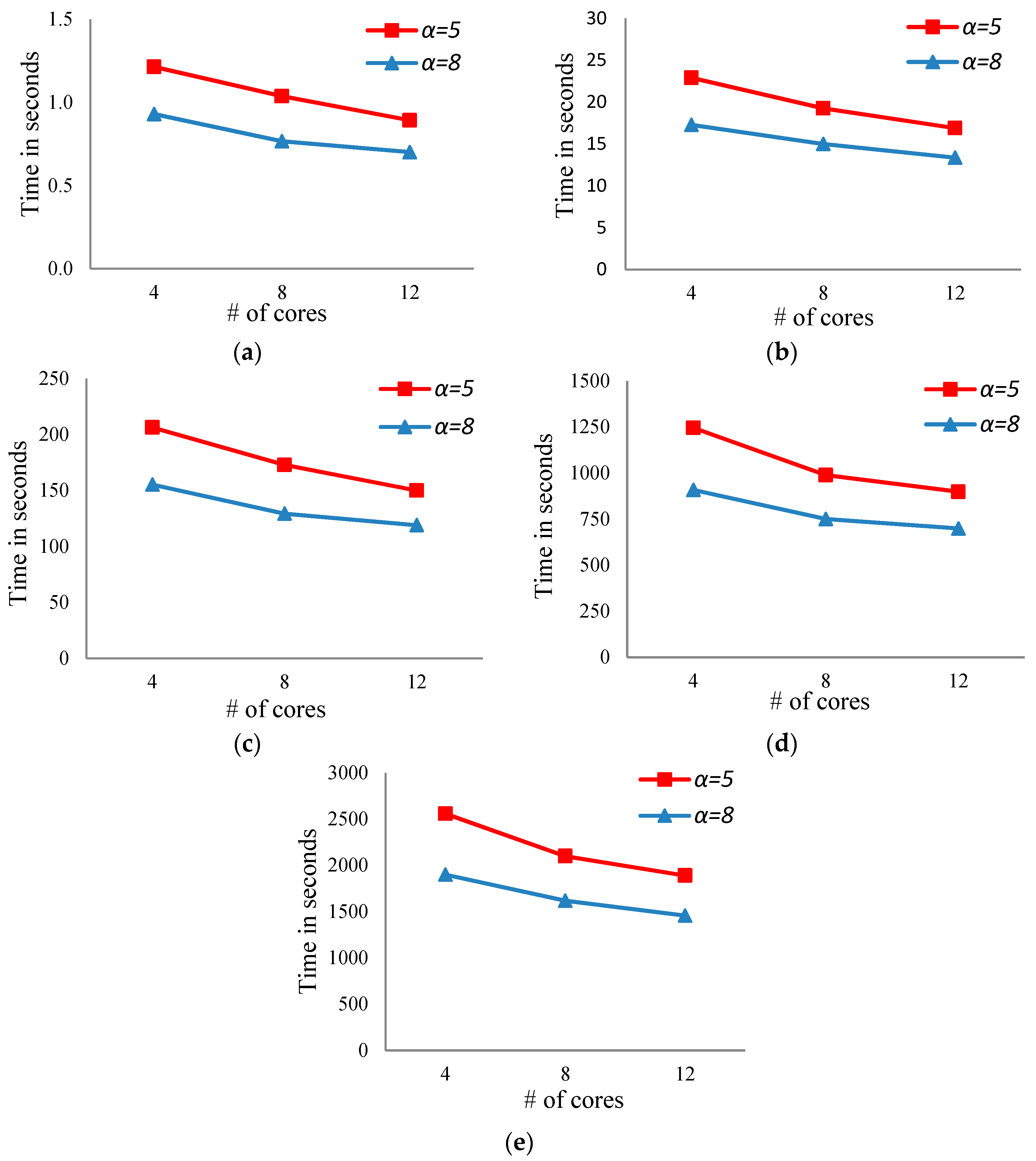
• For a fixed number of bits, the running time of the proposed algorithm decreases with increasing the number of cores (see Figure 3a–e).
• For a fixed number of bits, increasing the number of levels in the case of the breadth search will reduce the running time (see Figure 3a–e in both cases, α = 5 and 8).
• The running time of the proposed algorithm increases with increasing the number of bits (see Figure 4).
• Increasing the number of threads is effective when the number of bits is large. For example, in the case of 20 bits, the running time of the proposed algorithm using 4, 8, and 12 threads is 1245.4, 989.2, and 899.0 s, respectively, when α = 5.
• The time spent in the BF stage in the proposed algorithm is very small compared to the total running time. In the case of α = 5, the average time for breadth stage tends to zero, while in the case of α = 8, the average time for the breadth stage equals 0.03 s.
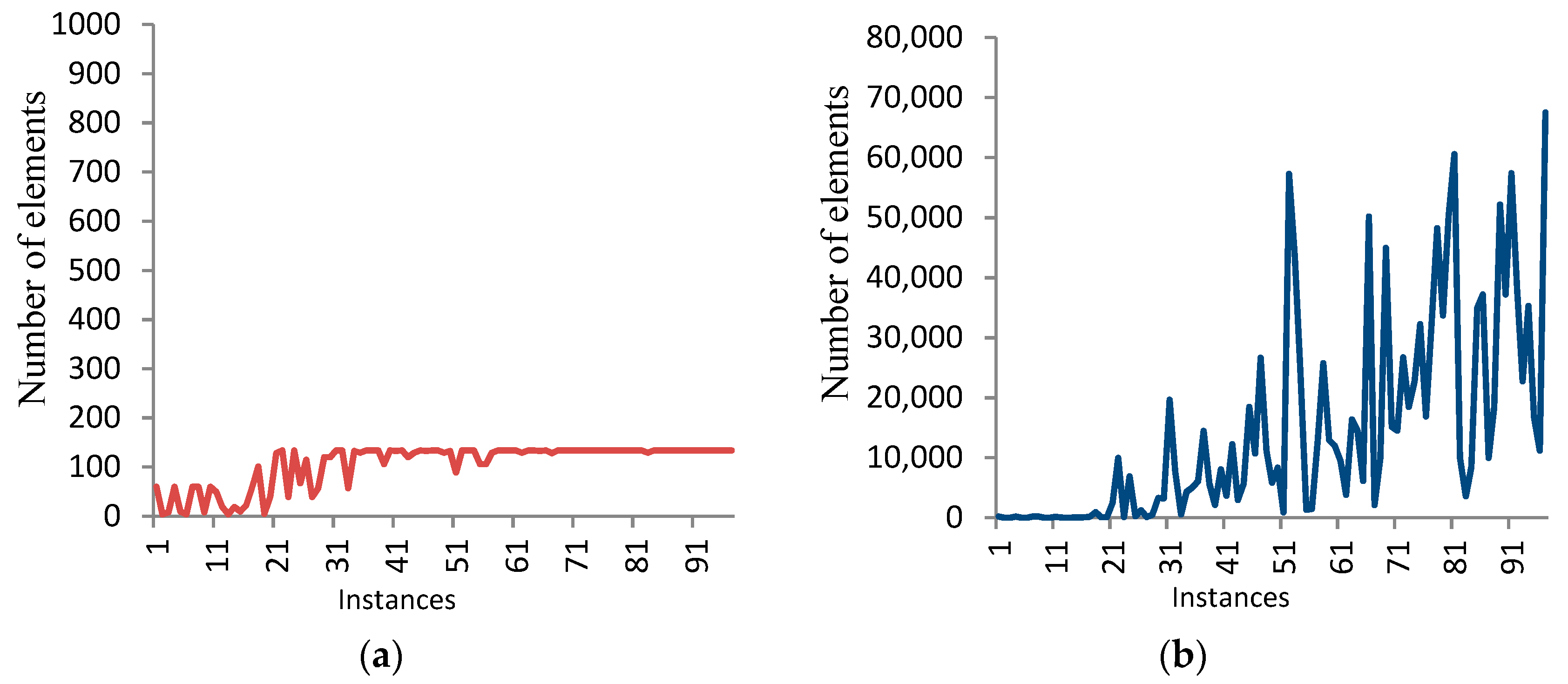
• The storage required by the BF stage increases when increasing the level α. Figure 5 shows the number of elements generated by the DF stage in the case of α = 5 and 8 for 100 numbers, each of 14 bits.
• The storage required by the DF stage increases with the increase of the number of bits in the average cases.

  Table 1. The size of the stack for the depth-first (DF) stage in the average case at α.

  α	Number of Bits
  	14	16	18	20	22
  5	45	57	66	78	89
  8	37	48	59	70	81

  shows this behavior in the average case. On the other side, the storage required by the DF stage decreases with the increase of the level α in the BF stage.
• The expected amount of memory required by the proposed algorithm is (|Q_α|$\times$(α + 1)) + Size(T) $\times$p, where Q_α is the queue that represents the list of all elements at level α, and T is the stack that represents the list of all elements in the DF search from level α+1 to Lb. The term (α + 1) represents the number of elements of the chain from level 0 to level α, while the term Size (T)$\times$p represents the size of stacks for all threads.
• The term (|Q_α| $\times$ (α + 1)) is very large compared to the term Size (T)$\times$p, so the storage required by the proposed algorithm increases with the increase of the level α in the average case.
• In some cases, we found that the running time of the sequential algorithm is less than or equal to the running time of the proposed algorithm when the number of 1s is very small or the goal exists in the left of the search space and the length of a minimal length chain is equal to the initial lower bound. For example, let m = 148,544 = (100100010001000000)₂. The running time of the sequential and proposed algorithms on m is 0.015 s. In addition, the running time for the sequential and proposed algorithms on m = 164560 = (101000001011010000)₂ is 0.015 and 0.031 s, respectively, using four threads in the case of parallelism.
• In general, the behavior of traversing the search tree is unsystematic in the sense that the running times for different numbers of the same size have a significant difference in some instances. For example, the running times for three different instances, each of 18 bits, are 23.75, 175.94, and 834.2 s. Also, the same behavior occurs for the memory consumed (see Figure 5).
• Table 2. The running time for the best known sequential algorithm to find the minimal length addition chain (MLAC).

  Number of bits	14	16	18	20	22
  Time in seconds	1.3	25.2	243.4	1556.8	3581.6

  shows the running time for the best known sequential algorithm to generate the MLAC using the same datasets. It is clear, from Table 2 and Figure 3, that the running time of the parallel proposed algorithm is faster than that of the sequential algorithm. For example, the running time for the best known sequential algorithm when m = 16 is 25.2 s, while the parallel proposed algorithm’s running time equals 22.9, 19.3, and 16.9 using p = 4, 8, and 12, respectively, in the case of α = 5. Additionally, for the same dataset, the running time for the proposed parallel algorithm decreases to 17.3, 15, and 13.3 using p = 4, 8, and 12, respectively, in the case of α = 8.
• Table 3. The speedup of the proposed algorithm using different numbers of cores and bits, where α = 5 and 8.

  Number of Bits	α = 5			α = 8
  	p = 4	p = 8	p = 12	p = 4	p = 8	p = 12
  14	1.05	1.23	1.43	1.37	1.67	1.82
  16	1.10	1.31	1.49	1.46	1.68	1.89
  18	1.18	1.41	1.62	1.57	1.88	2.05
  20	1.25	1.57	1.73	1.71	2.07	2.23
  22	1.40	1.71	1.90	1.89	2.21	2.46

  represents the speedup of the proposed algorithm, where the speedup of a parallel algorithm equals the ratio between the running time of the fastest sequential algorithm and the running time of the parallel algorithm.
• From Table 3, we observe that the speedup of the proposed algorithm increases in the following cases.
  Case 1: the number of threads and levels are fixed, while the number of bits is changed. For example, the speedup of the proposed algorithm for the number of bits 14 and 16 is 1.05 and 1.10, respectively, using the number of threads and levels equal to 4 and 5, respectively.
  Case 2: the number of bits and levels are fixed, while the number of threads is changed. For example, the speedup of the proposed algorithm using the number of threads 4, 8, and 12 is 1.37, 1.67, and 1.82, respectively, using the number of bits and levels equal to 14 and 8, respectively.
  Case 3: the number of threads and bits are fixed, while the number of levels is changed. For example, the speedup of the proposed algorithm using the number of levels 4 and 8 is 1.57 and 2.07, respectively, using the number of bits and threads equal to 20 and 8, respectively.
• There are many factors that affect the values of the scalability for the proposed parallel algorithm. These factors are:
  (i) In some instances, for a fixed number of bits, the running time of the sequential algorithm is less than that of the proposed algorithm due to the existence of the goal at the beginning of the search tree (the left of the tree).
  (ii) When the first thread finds the MLAC, it exits the loop after activating the cancellation. The remaining threads will not exit the loop immediately. They exit the loop after finishing their tasks. This case will increase the running time of the proposed algorithm.
  Clearly, doubling or tripling the numbers of processors will not necessarily cut the run time by 2 or 3, respectively, and so on.

5. Conclusions

In this paper, we have addressed one of the important problems in generating minimal length addition chains for a positive integer m, which is that the running time increases rapidly with v(m). We have introduced a new parallel algorithm that is based on traversing the search tree in a breadth-first manner followed by a depth-first search in the various cores and applying the pruning conditions to reduce the search space. The proposed algorithm was implemented on a machine of 12 cores using the C++ language that is supported by the OpenMP library. The experimental results show that the running time decreases with the increase in the number of cores and the number of levels in the breadth stage. The maximum speedup achieved by the proposed algorithm is 2.5 times that of the best known sequential algorithm.

References

- Knuth, D.E. The Art of Computer Programming: Seminumerical Algorithms; Addison-Wesley: Boston, MA, USA, 1973; Volume 2. [Google Scholar]
- Gordon, D.M. A Survey of fast exponentiation methods. J. Algorithms 1998, 27, 129–146. [Google Scholar] [CrossRef]
- Rivest, R.; Shamir, A.; Adleman, L. A method for obtaining digital signatures and public-key cryptosystems. Commun. ACM 1978, 21, 120–126. [Google Scholar] [CrossRef]
- Yen, S.M. Cryptanalysis of secure addition chain for SASC applications. Electron. Lett. 1993, 31, 175–176. [Google Scholar] [CrossRef]
- Bahig, H. Improved generation of minimal addition chains. Computing 2006, 78, 161–172. [Google Scholar] [CrossRef]
- Bahig, H. Star reduction among minimal length addition chains. Computing 2011, 91, 335–352. [Google Scholar] [CrossRef]
- Bahig, H. A fast optimal parallel algorithm for a short addition chain. J. Supercomput. 2018, 74, 324–333. [Google Scholar] [CrossRef]
- Bergeron, F.; Berstel, J.; Brlek, S. Efficient computation of addition chains. J. Théorie Nr. Bordx. 1994, 6, 21–38. [Google Scholar] [CrossRef]
- Bergeron, F.; Berstel, J.; Brlek, S.; Duboc, C. Addition chains using continued fractions. J. Algorithms 1989, 10, 403–412. [Google Scholar] [CrossRef]
- Clift, N. Calculating optimal addition chains. Computing 2011, 91, 265–284. [Google Scholar] [CrossRef]
- Cruz-Cortés, N.; Rodríguez-Henríquez, F.; Juárez-Morales, R.; Coello Coello, C.A. Finding Optimal Addition Chains Using a Genetic Algorithm Approach. In Computational Intelligence and Security. CIS 2005. Lecture Notes in Computer Science; Springer: Berlin/Heidelberg, Germany, 2005; Volume 3801, pp. 208–215. [Google Scholar]
- Flammenkamp, A. Integers with a small number of minimal addition chains. Discret. Math. 1999, 205, 221–227. [Google Scholar] [CrossRef]
- Scholz, A. Jahresbericht: Deutsche Mathematiker Vereinigung. Aufgabe 1937, 47, 41–42. [Google Scholar]
- Thurber, E. Addition chains—An erratic sequence. Discret. Math. 1993, 122, 287–305. [Google Scholar] [CrossRef]
- Thurber, E. Efficient generation of minimal length addition chains. SIAM J. Comput. 1999, 28, 1247–1263. [Google Scholar] [CrossRef]
- Bleichenbacher, D.; Flammenkamp, A. An Efficient Algorithm for Computing Shortest Addition Chains. unpublished. Available online: http://www.homes.uni-bielefeld.de/achim/addition_chain.html (accessed on 21 May 2018).
- Chin, Y.; Tsai, Y. Algorithms for finding the shortest addition chain. In Proceedings of the National Computer Symposium, Kaoshiung, Taiwan, 20–22 December 1985; pp. 1398–1414. [Google Scholar]
- Fathy, K.; Bahig, H.; Bahig, H.; Ragb, A. Binary addition chain on EREW PRAM. In Proceedings of the International Conference on Algorithms and Architectures for Parallel Processing (ICA3PP 2011), Melbourne, Australi, 24–26 October 2011; Springer: Berlin/Heidelberg, Germany, 2011; Volume 7017, pp. 321–330. [Google Scholar]
- Schonhage, A.; Strassen, V. Schnelle multiplikation GroBer Zahlen. Computing 1971, 7, 281–292. [Google Scholar] [CrossRef]