Article

Parallel Computation of Rough Set Approximations in Information Systems with Missing Decision Data

1
Information Science and Control Engineering, Nagaoka University of Technology, Nagaoka 9402137, Japan
2
Human Machine Interaction Laboratory, UET, Vietnam National University, Hanoi 10000, Vietnam
*
Author to whom correspondence should be addressed.
Computers 2018, 7(3), 44; https://doi.org/10.3390/computers7030044
Submission received: 21 July 2018 / Revised: 12 August 2018 / Accepted: 16 August 2018 / Published: 20 August 2018

Abstract

:
The paper discusses the use of parallel computation to obtain rough set approximations from large-scale information systems where missing data exist in both condition and decision attributes. To date, many studies have focused on missing condition data, but very few have accounted for missing decision data, especially in enlarging datasets. One of the approaches for dealing with missing data in condition attributes is named twofold rough approximations. The paper aims to extend the approach to deal with missing data in the decision attribute. In addition, computing twofold rough approximations is very intensive, thus the approach is not suitable when input datasets are large. We propose parallel algorithms to compute twofold rough approximations in large-scale datasets. Our method is based on MapReduce, a distributed programming model for processing large-scale data. We introduce the original sequential algorithm first and then the parallel version is introduced. Comparison between the two approaches through experiments shows that our proposed parallel algorithms are suitable for and perform efficiently on large-scale datasets that have missing data in condition and decision attributes.

1. Introduction

Rough set theory (RST), first introduced by Pawlak [1,2], is a powerful mathematical tool to deal with inconsistency in datasets. RST has become one of the crucial and effective methods for feature selection [3,4,5,6], decision-making problems [7,8,9,10,11], pattern recognition [12,13], data mining and knowledge acquisition [14,15,16,17,18,19,20,21].
Data analysis in RST starts from a data table named information system. Each row of the table induces a decision rule, which specifies a decision (action, result, outcome, etc.) if some conditions are satisfied. The original RST presupposes that all the condition and decision data in the information system are complete. However, incomplete (i.e., missing) data is often seen in real applications due to many reasons. It occurs not only in conditions but also in the decision attribute. For example, if an information system contains data on symptoms and diseases of patients in a hospital, some decision data may be missing when the patients stop seeking treatment, e.g., for financial reasons. Furthermore, decision data may be blank owing to an inadvertent erasure or for reasons of privacy. A common approach might be to remove such objects with missing decision data. However, in our previous work [22,23], we gave evidence that removing such objects may lead to information loss. For example, the removal may change the original data distribution, break relations between condition attributes, or the induced knowledge after the removal would be different from the knowledge in the original information system where those objects are retained. Clearly, such objects with missing decision data should not be removed or should be handled in an appropriate way.
Recently, with the emerging era of big data, new RST-based approaches have been studied to deal with large-scale datasets [5,18,24,25,26,27,28,29,30,31,32,33,34,35]. This study is inspired by the introduction of MapReduce framework [36] for processing intensive datasets, and the fact that most of algorithms on small-scale datasets did not perform well on large-scale datasets. As we observed, all of the above MapReduce-based studies aim for large-scale information systems with no missing data, or with missing data only in condition attributes. To the best of our knowledge, there was no study on large-scale information systems in which some of the data, both in conditions and the decision, are missing. Inspired from this shortage, we propose a parallel method to compute rough approximations in such massive, incomplete condition and decision information systems.
Our proposed method is motivated from the method twofold rough approximations, which was introduced by Sakai et al. [37]. The method of twofold rough approximations was originally designed for information systems which contain missing data only in condition attributes. In this paper, we extend the method for information systems which contain missing data in both conditions and decision attributes. In addition, using sequential algorithms to computing twofold rough approximations in such information systems is time consuming, and even impossible. Hence, we propose parallel algorithms to accelerate the computation in such massive, incomplete condition and decision information systems.
The rest of the paper is organized as follows. Section 2 reviews some related studies in the literature. Section 3 summarizes basic concepts of RST, MapReduce model and the usage of MapReduce to accelerate rough set processing. Section 4 introduces the method of twofold rough approximations and how to apply it to information systems with missing condition and decision data. Section 5 introduces the sequential algorithm and MapReduce-based parallel algorithms to compute twofold rough approximations in large-scale information systems. Evaluation tests are presented at the end of this section. The paper ends with conclusions in Section 6.

2. Literature Review

On small-scale datasets, problems on missing condition values have been studied extensively and have achieved positive results [38,39,40,41,42,43,44,45,46,47,48,49,50,51,52,53,54,55,56,57,58,59,60,61]. Some authors attempted to transform an incomplete information system to a complete information system by: removing objects with missing condition values; treating them as special values; replacing them with average values, with most common values, or with all possible values [42,44]. Others extended the concept of classical equivalence relation by relaxing the requirements of reflexivity, symmetry, and transitivity. This created new binary relations such as tolerance relation [50,51], valued tolerance relation [48], maximal consistent block [52], similarity relation [47], difference relation [60], limited tolerance relation [59], characteristic relation [43,46], etc. By considering the weaknesses of the tolerance and similarity relations, Sakai et al. [37] introduced the method of possible worlds and twofold rough approximations. The latter proved its accuracy since it gave the same rough approximations as the former while more computational efficiency. Not only in conditions, missing data can appear in the decision attribute. To deal with the issue of missing decision data, Medhat [62] suggested a method to restore missing decision data by measuring the similarity distance between objects with and without missing decision data. However, his method requires all the condition data to be complete, which is also rare in practice. A common approach to deal with such objects with missing decision data is to remove them. In our previous studies, however, we proved that removing such objects may lead to information loss [22,23]. Hence, instead of removing such objects, we proposed a parameter-based method to induce knowledge from such information system. Our proposed method offered a more generalized approach to handle missing decision data without having to remove them, thus minimizing the threat of information loss.
Recently, with the emerging era of big data, new RST-based approaches have been studied to deal with large-scale datasets [5,18,24,25,26,27,28,29,30,31,32,33,34,35]. Basically, two approaches are employed to speed up the process of knowledge acquisition in big datasets. Incremental approach is an effective mechanism to discover knowledge from a gradually increasing dataset [5,18,24,31,32,33,34,35]. It uses different learning techniques to avoid re-calculating approximation sets [18,24,31,32,34], reducts, or rules [5,33,35] from scratch, thus reducing the computation time.
Parallel programming [25,26,27,28,29,30,63] is another approach to accelerate the process of knowledge acquisition. Most of the methods in this approach are based on MapReduce. MapReduce, introduced by Google (CA, US) [36], is a software framework to support processing large data on clusters of computers. MapReduce framework has proved its efficiency since it has been widely used in data mining [64,65], machine learning [66,67,68,69] and web indexing [70]. Based on MapReduce, Zhang [25] proposed a parallel method to effectively compute set approximations. He also implemented algorithms on different MapReduce runtime systems such as Hadoop, Phoenix, and Twister to compare the knowledge extracted from these systems [26]. Li et al. [71] was one of the earliest authors using MapReduce for attribute reduction. The proposed approach divided the original datasets into many small data blocks, and used reduction algorithms for each block. Then, the dependency of each reduction on testing data was computed in order to select the best reduction. Qian et al. [30] proposed a hierarchical approach for attribute reduction. He designed the parallel computations of equivalence classes and attribute significance, as a result, the reduction efficiency was significantly improved. In [29], Qian et al. proposed three parallelization strategies for attribute reduction, namely “Task-Parallelism”, “Data-Parallelism”, and “Data+Task-Parallelism”. El-Alfy et al. [63] introduced a parallel genetic algorithm to approximate the minimum reduct and applied it to intrusion detection in computer networks. Li and Chen [27,28] computed set approximations and reducts in parallel using dominance-based neighborhood rough sets, which considers the orders of numerical and categorical attribute values. Some authors studied rough sets in large-scale datasets with missing condition data [72,73]. Zhang [72] designed a parallel matrix-based method to compute rough approximations in large-scale information systems with some condition values being missing. Based on complete tolerance class, Yuan [73] proposed an algorithm to fill the missing condition values of energy big data.

3. Basic Concepts

In this section, we review basic concepts of rough sets [1,2] and MapReduce technique [36].

3.1. Rough Set

An information system (IS) in the rough set study is formally described as ξ = ( U , A T { d } , V , f ) , where U is a non-empty set of objects, A T is a non-empty set of condition attributes, d A T denotes a decision attribute, f is an information function f : U × A T { d } V , V = V t for any t A T { d } . f ( x , a ) and f ( x , d ) , x U , a A T are represented by f a ( x ) and f d ( x ) , respectively. V a and V d denote the domain of f a and f d , respectively. Any domain may contain special symbols “∗” to indicate a missing value, i.e., the value of an object is unknown. Any value different from “∗” will be called regular [52]. We use complete information system (CIS) to denote an IS with no missing values, incomplete information system (IIS) to denote an IS where missing values are just only in the condition attributes, and incomplete decision system (IDS) to denote an IS where missing values are both in condition and decision attributes.
The RST is formed on the basic of equivalence relation. Two objects are equivalent on A A T if and only if their corresponding values are equal on every attribute in A, denoted by E Q R ( A ) . Formally, E Q R ( A ) = { ( x , y ) U × U | a A , f a ( x ) = f a ( y ) } . The equivalence relation is reflexive, symmetric, and transitive. An equivalence relation divides U into a partition, given by U / E Q R ( A ) = { E A ( x ) | x U } . U / E Q R ( A ) is normally denoted by U / A for simplicity. Let  E A ( x ) = { y U | ( x , y ) E Q R ( A ) } be a set of objects equivalent to x w.r.t. A, and be called the equivalence class of x w.r.t. A.
Let X U be a set of objects with regular decision values, called a target set. The lower approximation of X w.r.t A is defined by R ̲ A ( X ) = { x U | E A ( x ) X } . The upper approximation of X w.r.t A is defined by R ¯ A ( X ) = { x U | E A ( x ) X } . If boundary region of X , i.e., B N D A ( X ) = R ¯ A ( X ) R ̲ A ( X ) is not empty, the pair ( R ¯ A ( X ) , R ̲ A ( X ) ) is called a rough set.

3.2. MapReduce Model

MapReduce is a software framework to implement parallel algorithms [36]. It is designed to handle large-scale datasets in a distributed environment. In MapReduce model, the computation is divided into two phases: Map and Reduce. These phases are performed in order, i.e., the Map phase is executed first and then the Reduce phase is executed. The output of Map phase is used as input of the Reduce phase. We implement these phases through Map and Reduce functions, respectively. Each function requires a pair key/value as input and another pair key/value as output. The Map and Reduce functions are illustrated as follows:
M a p : < K 1 , V 1 > [ < K 2 , V 2 > ] ,
R e d u c e : < K 2 , [ V 2 ] > [ < K 3 , V 3 > ] ,
where K i , V i , i = { 1 , 2 , 3 } are user-defined data types and [ . . ] denotes a set of the element in the square bracket.
Map takes an input pair ( < K 1 , V 1 > ) and produces a set of intermediate key/value pairs ( [ < K 2 , V 2 > ] ). The MapReduce library groups all intermediate values associated with the intermediate key K 2 , shuffles, sorts, and sends them to the Reduce function. Reduce accepts an intermediate key ( K 2 ) and a set of values for that key ( [ V 2 ] ). It merges these values together to create a possibly smaller set of values, and finally produces < K 3 , V 3 > pairs as output.
One of the primary advantages of MapReduce framework is that it splits tasks so that their execution can be done in parallel. Since these divided tasks are processed in parallel, this allows the entire task to be executed in less time. In addition, MapReduce is easy to use because it hides many system-level details from programmers such as parallelization, fault-tolerance, locality optimization, and load balancing. In practice, to use the MapReduce model, what programmers need to do is to design proper < k e y , v a l u e > pairs and implement Map/Reduce functions.

3.3. The Usage of MapReduce to Rough Set Processing

It is possible to use MapReduce to speed up Rough set processing. One of the earliest implementation was done by Zhang [25]. Using MapReduce, he ran several steps in parallel such as computing equivalence classes, decision classes and associations between equivalence classes and decision classes. He proved that rough set approximations obtained by the parallel method are the same as those obtained by the sequential method but the former takes less time than the latter.
Let’s examine how equivalence classes can be computed in parallel. Let ξ = ( U , A T { d } , V , f ) be an CIS, and U / A = { E A 1 , E A 2 , . . , E A m } . In MapReduce platform, ξ is divided into k sub-CIS, e.g., ξ 1 , ξ 2 , . . . , ξ k , where ξ i = ( U i , A T { d } , V , f ) , i = { 1 , 2 , . . , k } s.t. U i = . In Map step, we partition each ξ i into equivalence classes, and then these equivalent classes are aggregated in a Reduce step. Note that there will be k numbers of mappers running in parallel, and each mapper will execute Map function to process corresponding ξ i :
Maps output:
Map 1: < E A 11 , v 11 > , < E A 12 , v 12 > , . . , < E A 1 m , v 1 m > , where U 1 / A = { E A 11 , E A 12 , . . , E A 1 m } .
Map 2: < E A 21 , v 21 > , < E A 22 , v 22 > , . . , < E A 2 m , v 2 m > , where U 2 / A = { E A 21 , E A 22 , . . , E A 2 m } .
Map k: < E A k 1 , v k 1 > , < E A k 2 , v k 2 > , . . , < E A k m , v k m > , where U k / A = { E A k 1 , E A k 2 , . . , E A k m } .
In the above, E A k m represents the m th equivalence class w.r.t. A on the sub-CIS U k , and v k m represents a set of objects that belong to E A k m .
Reducers output:
Reduce 1: < E A 1 , v 1 = v 11 v 21 . . . v k 1 > ,
Reduce 2: < E A 2 , v 2 = v 12 v 22 . . . v k 2 > ,
Reduce m: < E A m , v m = v 1 m v 2 m . . . v k m > .
As we observe, computing U / A = { E A 1 , E A 2 , . . , E A m } in sequence costs O ( | U | | A | ) time complexity while doing the same in parallel costs just O ( | U | | A | / k ) time complexity. Clearly, computational time is reduced using the MapReduce platform. This shows the strength of the MapReduce platform in increasing performance of Rough set computation.

4. Twofold Rough Approximations for IDS

In this section, we discuss the usage of twofold rough approximations in the case of missing condition and decision data.
Sakai et al. [37] introduced the method of twofold rough approximations to deal with missing data in condition attributes. He pointed out that, when an IS contains incomplete information, we can not derive unique rough approximations but can only derive lower and upper bounds of the actual rough approximation. He refers to the lower and upper bounds as certain and possible rough approximations, hence the name twofold rough approximations. The rough approximations obtained from this method coincide with ones from the method of possible worlds.
The method is based on an idea of considering both aspects (discernibility and indiscernibility) of every missing value. For example, let us assume an IIS with two objects x , y whose values on a A are f a ( x ) and ∗, respectively. Since the missing value may equal f a ( x ) (or not), x may be indistinguishable (or distinguishable) from y on a. Because we do not know the exact value of ∗, we should consider these both cases. Thus, we should take { x } , { y } and { x , y } into account since they have the possibility that each of them is the actual equivalence class w.r.t a. The set { { x } , { y } , { x , y } } is called possible equivalence classes.
The same interpretation can also apply for missing value in the decision. Given object z with f d ( z ) = , the above interpretation suggests that f d ( z ) may be any value in the decision domain. Since we do not know the exact value of f d ( z ) , we need to consider all the possibilities. In the following, we describe the usage of twofold rough approximations for IDS.
Let ξ = ( U , A T { d } , V , f ) be an IDS. For each a A T , we can divide the universe U into two sets U a = and U a representing objects whose values on attribute a are missing and regular respectively. Let U a / a be a partition of U a by a. We define C e r ( U / a ) , P o s ( U / a ) as certain and possible equivalence classes w.r.t a respectively. Formally,
C e r ( U / a ) = U a / a { } , P o s ( U / a ) = { e U a = | e U a / a } { U a = } .
Let X be a target set. Unlike the original definition of target set, here we define X is a family of equivalence classes w.r.t. the decision d included in U d , i.e., X = U d / d = { X 1 , X 2 , . . , X m } . X might be called a family of certain equivalence classes w.r.t. the decision d, denoted as X C e r . We also define X P o s as a family of the possible equivalence classes w.r.t. the decision d, each of which is a union of a certain equivalence class and U d = . U d = itself is also included in the family. Formally,
X C e r X , X P o s = { e U d = | e X } { U d = } .
C e r ( U / A ) , P o s ( U / A ) are defined as the family of certain and possible equivalence classes w.r.t. A A T , respectively:
C e r ( U / A ) = { i e a i j | e a i j C e r ( U / a i ) , a i A } , P o s ( U / A ) = { i e a i j | e a i j P o s ( U / a i ) , a i A } .
The certain lower and upper approximations of X w.r.t. A:
R ̲ A C e r ( X ) = { i e i | e i r ̲ A C e r ( x ) , x X C e r } , R ¯ A C e r ( X ) = { i e i | e i r ¯ A C e r ( x ) , x X C e r } ,
where
r ̲ A C e r ( x ) = { e | e e , e x , e C e r ( U / A ) , e P o s ( U / A ) } , r ¯ A C e r ( x ) = { e | e C e r ( U / A ) , e x } .
The possible lower and upper approximations of X w.r.t. A:
R ̲ A P o s ( X ) = { i e i | e i r ̲ A P o s ( x ) , x X P o s } , R ¯ A P o s ( X ) = { i e i | e i r ¯ A P o s ( x ) , x X P o s } ,
where
r ̲ A P o s ( x ) = { e x | e e , e x , e P o s ( U / A ) , e C e r ( U / A ) } , r ¯ A P o s ( x ) = { e | e P o s ( U / A ) , e x } .
Example 1.
Given an IDS as in Table 1, where a 1 , a 2 A are condition attributes, d is the decision attribute. Let X = U d / d = { { x 1 , x 5 , x 7 } , { x 2 } , { x 3 , x 6 } , { x 8 } } , and U d = = { x 4 } . Then, X C e r = X , X P o s = { { x 1 , x 4 , x 5 , x 7 } , { x 2 , x 4 } , { x 3 , x 4 , x 6 } , { x 4 , x 8 } , { x 4 } } . Results are shown in Table 2, Table 3 and Table 4.
From Table 2: C e r ( U / A ) = { , { x 5 } , { x 1 , x 4 } , { x 8 } } , P o s ( U / A ) = { , { x 2 } , { x 7 } , { x 2 , x 8 } , { x 3 , x 6 } , { x 2 , x 3 , x 6 } , { x 3 , x 6 , x 7 } , { x 2 , x 5 } , { x 1 , x 4 , x 7 } } .
From Table 3: R ̲ A C e r ( X ) = , R ¯ A C e r ( X ) = { { x 8 } , { x 5 } , { x 1 , x 4 } } .
From Table 4: R ̲ A P o s ( X ) = { { x 2 } , { x 4 } , { x 5 } , { x 7 } , { x 8 } , { x 3 , x 6 } , { x 1 , x 4 , x 7 } } , R ¯ A P o s ( X ) = { { x 2 } , { x 7 } , { x 2 , x 5 } , { x 2 , x 8 } , { x 3 , x 6 } , { x 2 , x 3 , x 6 } , { x 3 , x 6 , x 7 } , { x 1 , x 4 , x 7 } } .

5. Computing Rough Approximations in IDS

In this section, we give the sequential algorithm and MapReduce-based parallel algorithm to compute twofold rough approximations in IDS.

5.1. Sequential Algorithm

Algorithm 1 describes the sequential algorithm to compute twofold rough approximations. The algorithm consists of four steps. For each a A , we calculate a partition U a / a , then certain and possible equivalence classes on a, i.e., C e r ( U / a ) and P o s ( U / a ) (Step 1). These C e r ( U / a ) and P o s ( U / a ) are then aggregated together to form C e r ( U / A ) and P o s ( U / A ) (Step 2). Next, we compute X C e r , X P o s where X represents the target set (Step 3). Lastly, we calculate twofold rough approximations (Step 4).
Algorithm 1 Sequential algorithm to calculate twofold rough approximations
Computers 07 00044 i001
Let us analyze the computational complexity of Algorithm 1. Let n be the number of objects in U, and m be the number of attributes, i.e., n = | U | , m = | A | . If we assume that the number of partition equals the number of objects in the worst case, the order of computation of U / a is O ( n ) , thus Step 1 costs O ( n m ) . In Step 2, we compute C e r ( U / A ) and P o s ( U / A ) , which is required to compute the Cartesian product between C e r ( U / a ) and P o s ( U / a ) . Since C e r ( U / a ) or P o s ( U / a ) costs O ( n ) , Step 2 costs O ( n m ) in total. We compute X C e r and X P o s s in Step 3, whose time complexity is O ( n ) . In Step 4, the computation order of R ̲ A P o s ( X ) , R ̲ A C e r ( X ) is O ( n 3 ) while the one of R ¯ A P o s ( X ) , R ¯ A C e r ( X ) is O ( n 2 ) . Thus, Step 4 costs O ( n 3 ) at worst. In total, the overall complexity of Algorithm 1 is dominated by Step 2, which is O ( n m ) . This overall complexity is intensive for large datasets where n and m are large. For a more efficient computation, we introduce an approach to process Step 2 in parallel. In addition, other computation-intensive steps are also performed in parallel in order to reduce the whole computation time.

5.2. MapReduce Based Algorithms

The sequential approach may take a lot of time to compute rough approximations, especially when input data are large. Using MapReduce, we speed up the computation by implementing the parallel algorithm for all the above steps. The flow of the parallel algorithm is illustrated in Figure 1.
We divide into four sub-algorithms: computing equivalence classes (EC), computing possible and certain equivalence classes (PEC), computing aggregation of possible and certain equivalence classes (AP), and computing twofold rough approximations (RA). We examine each algorithm in the following.

5.2.1. Computing Equivalence Classes in Parallel (EC)

Let ξ = ( U , A T { d } , V , f ) be an IDS, A A T . Let ξ = i = 1 k ξ i , ξ i = ( U i , A T { d } , V , f ) where U i = and U = i = 1 k U i . It means the original IDS is divided into k sub-IDS. Assume that domain of a A is the same between these IDS, i.e., V a i = V a , i { 1 , 2 , . . k } .
Proposition 1.
For a A , let X a i ( v ) = { x i U i | f a ( x i ) = v , v V a i } and X a ( v ) = { x U | f a ( x ) = v , v V a } . Then, X a ( v ) = X a i ( v ) .
Proof. 
⟹ Suppose y X a ( v ) = { x U | f a ( x ) = v , v V a } . Because U = i = 1 k U i , U i s.t. y U i , f a ( y ) = v , v V a i , i.e., y X a i ( v ) .⟸ Suppose y X a i ( v ) , i.e., X a i ( v ) such that y { x i U i | f a ( x i ) = v , v V a i } . Since U i U and V a i = V a , y { x i U | f a ( x i ) = v , v V a } = X a ( v )  ☐
Example 2.
Let us divide the data in Table 1 into two sub-IDS ξ 1 , ξ 2 (Table 5). Suppose V a 1 = V a 1 1 = V a 1 2 = { 1 , 2 , 3 } .
From ξ 1 : X a 1 1 ( 1 ) = { x 1 , x 4 } , X a 1 1 ( 2 ) = { x 3 } , X a 1 1 ( 3 ) = , X a 1 1 ( ) = { x 2 } ,
From ξ 2 : X a 1 2 ( 1 ) = { x 5 } , X a 1 2 ( 2 ) = { x 6 } , X a 1 2 ( 3 ) = { x 8 } , X a 1 2 ( ) = { x 7 } ,
From Table 1: X a 1 ( 1 ) = { x 1 , x 4 , x 5 } , X a 1 ( 2 ) = { x 3 , x 6 } , X a 1 ( 3 ) = { x 8 } , X a 1 ( ) = { x 2 , x 7 } .
We have X a 1 ( 1 ) = X a 1 1 ( 1 ) X a 1 2 ( 1 ) , X a 1 ( 2 ) = X a 1 1 ( 2 ) X a 1 2 ( 2 ) , X a 1 ( 3 ) = X a 1 1 ( 3 ) X a 1 2 ( 3 ) , X a 1 ( ) = X a 1 1 ( ) X a 1 2 ( ) .
Note that U a / a = { X a ( v ) | v V a } = { E a ( x ) | x U , f a ( x ) = v V a } . Hence, the above proposition implies that equivalence classes on each attribute a A can be computed in parallel. We design the EC Map and EC Reduce functions as follows.
Algorithm 2 function EC Map
Computers 07 00044 i002
Algorithm 3 function EC Reduce
Computers 07 00044 i003
The input of the EC Map is a data split ξ i . For each attribute a, and each object x i U i , we output intermediate pairs < k e y , v a l u e > where k e y is a tuple ( a , f a ( x i ) ) and v a l u e is the object x i  itself. The MapReduce framework copies objects x i with the same k e y from different mapper nodes to corresponding reducer nodes. The EC Reduce accepts ( a , f a ( x i ) ) as input key, and a list of x i as input values. We aggregate this list of x i to form X a ( v ) .
Example 3.
(Example 2 continued) The output of EC Map: Map1: < ( a 1 , 1 ) , x 1 > , < ( a 2 , 2 ) , x 1 > < ( a 1 , ) , x 2 > < ( a 2 , 1 ) , x 2 > , < ( a 1 , 2 ) , x 3 > , < ( a 2 , ) , x 3 > , < ( a 1 , 1 ) , x 4 > , < ( a 2 , 2 ) , x 4 > .
Map2: < ( a 1 , 1 ) , x 5 > , < ( a 2 , 1 ) , x 5 > , < ( a 1 , 2 ) , x 6 > , < ( a 2 , ) , x 6 > , < ( a 1 , ) , x 7 > , < ( a 2 , 2 ) , x 7 > , < ( a 1 , 3 ) , x 8 > , < ( a 2 , 1 ) , x 8 > .
The output of EC Reduce: < ( a 1 , ) , ( x 2 , x 7 ) > , < ( a 1 , 1 ) , ( x 1 , x 4 , x 5 ) > , < ( a 1 , 2 ) , ( x 3 , x 6 ) > , < ( a 1 , 3 ) , x 8 > , < ( a 2 , ) , ( x 3 , x 6 ) > , < ( a 2 , 1 ) , ( x 2 , x 5 , x 8 ) > , < ( a 2 , 2 ) , ( x 1 , x 4 , x 7 ) > .

5.2.2. Computing Possible and Certain Equivalence Classes in Parallel (PEC)

In this part, we compute possible and certain equivalence classes on each attribute a A following Equation (1).
Proposition 2.
For a A , C e r ( U / a ) = C e r ( U i / a ) and P o s ( U / a ) = P o s ( U i / a ) .
Proof. 
C e r ( U / a ) = C e r ( U i / a ) is directly from Proposition 1 and Equation (1). For P o s ( U / a ) , P o s ( U / a ) = { e U a = | e U a / a } { U a = } = { e U a = i | e U a i / a } { U a = i } = { { e U a = i | e U a / a } { U a = i } } = P o s ( U i / a )  ☐
The proposition proves that the certain and possible equivalence classes on each attribute can be computed in parallel. The PEC Map and PEC Reduce functions are designed as follows:
Algorithm 4 function PEC Map
Computers 07 00044 i004
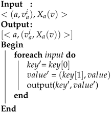
This step is executed right after the previous step, so it uses the direct output of EC Reduce as input. An input key of PEC Map is in the form ( a , v a i ) . We extract the first element of the input key to be our intermediate key. The second element of the input key combined with the input value creates our intermediate values. The MapReduce platform groups all intermediate values w.r.t an intermediate key (i.e., an attribute) and sends them to corresponding reducers.
The PEC Reducer accepts the intermediate pairs and loop over the intermediate values. c m i s s i n g  is used to represent objects whose values are missing while c r e g u l a r is a set of subsets, each subset contains objects whose values are regular. Then, we calculate certain equivalence classes c c e r and possible equivalence classes c p o s according to Formula (1). When c m i s s i n g is empty, both c c e r and c p o s are equal c r e g u l a r . The output is < k e y , ( c c e r , c p o s ) > , where k e y represents an attribute, c c e r , c p o s represent certain and possible equivalence classes on the attribute, respectively.
Algorithm 5 function PEC Reduce
Computers 07 00044 i005
Example 4.
(Example 3 continued) The output of PEC Map:
< a 1 , ( , { x 2 , x 7 } ) > , < a 1 , ( 1 , { x 1 , x 4 , x 5 } ) > , < a 1 , ( 2 , { x 3 , x 6 } ) > , < a 1 , ( 3 , { x 8 } ) > ,
< a 2 , ( , { x 3 , x 6 } ) > , < a 2 , ( 1 , { x 2 , x 5 , x 8 } ) > , < a 2 , ( 2 , { x 1 , x 4 , x 7 } ) > .
The output of PEC Reduce:
< a 1 , ( c c e r , c p o s ) > , where c c e r = { , { x 1 , x 4 , x 5 } , { x 3 , x 6 } , { x 8 } } , c p o s = { , { x 2 , x 7 } , { x 2 , x 7 , x 8 } , { x 1 , x 2 , x 4 , x 5 , x 7 } , { x 2 , x 3 , x 6 , x 7 } } .
< a 2 , ( c c e r , c p o s ) > , where c c e r = { , { x 2 , x 5 , x 8 } , { x 1 , x 4 , x 7 } } , c p o s = { , { x 3 , x 6 } , { x 2 , x 3 , x 5 , x 6 , x 8 } , { x 1 , x 3 , x 4 , x 6 , x 7 } } .

5.2.3. Aggregating Possible and Certain Equivalence Classes in Parallel (AP)

In this part, we aggregate in parallel the certain and possible equivalence classes on a set of attributes A A T , following Equation (3).
Let us divide A into smaller subsets A t where A t = and A = t A t . The following propositions hold:
Proposition 3.
For A t A , let C e r ( U / A t ) = { i e a i j | e a i j C e r ( U / a i ) , a i A t } and C e r ( U / A ) = { i e a i j | e a i j C e r ( U / a i ) , a i A } . Then, C e r ( U / A ) = C e r ( U / A t ) .
Proof: e C e r ( U / A ) e { i e a i j | e a i j C e r ( U / a i ) , a i t A t } e t { i e a i j | e a i j C e r ( U / a i ) , a i A t } e C e r ( U / A t ) .
Proposition 4.
For A t A , let P o s ( U / A t ) = { i e a i j | e a i j P o s ( U / a i ) , a i A t } and P o s ( U / A ) = { i e a i j | e a i j P o s ( U / a i ) , a i A } . Then, P o s ( U / A ) = P o s ( U / A t ) .
Proof. 
Similar to proof of Proposition 3. ☐
The above propositions prove that the aggregation of certain and possible equivalence classes can also be executed in parallel. To avoid memory overhead, we separate the process of aggregating certain equivalence classes from the process of aggregating possible equivalence classes. For aggregating certain equivalence classes, we extract only c c e r from the output of PEC Reduce and vice versa. Algorithms 6 and 7 illustrate the process of aggregating certain equivalence classes.
Algorithm 6 function AP Map
Computers 07 00044 i006
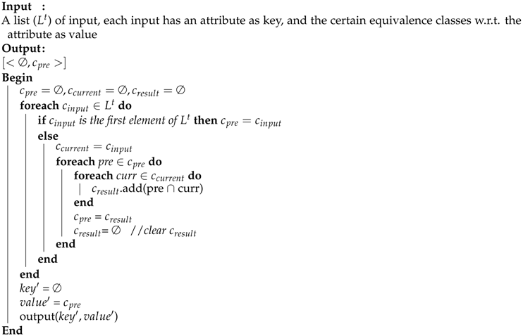
Both algorithms are identical: they receive a list of certain equivalence classes and produce the intersection between these certain equivalence classes. Given a list of certain equivalence classes L t , the intersections of elements of L t can be computed sequentially. That is, intersections between the first and second elements of L t will be computed first; then, the result is used to find intersections with the third element of L t . The process repeats until the last element of L t . We denote c p r e as a variable to contain the intersections of previous elements, c c u r r e n t to contain current element, and c r e s u l t to contain the intersections between c p r e and c c u r r e n t . In the end, c p r e contains the intersections of all elements in  L t . In AP Reducer, we collect all c p r e from different nodes, and repeat the above process to compute the intersections between them. The final outputs are the intersections of certain equivalence classes of all attributes.
Since the process of aggregating possible equivalence classes is identical to the process of aggregating certain equivalence classes, the above AP Map and AP Reduce functions can also be used. The difference is the input of AP Map: instead of certain equivalence classes of each attribute ( c c e r ), we use possible equivalence classes ( c p o s ).
To avoid computation overhead, this AP step can be divided into multiple MapReduce jobs. However, in order to get the final intersection, we need to set the number of reducers of the last MapReduce job as 1.
Algorithm 7 function AP Reduce
Computers 07 00044 i007
Example 5.
(Example 4 continued) To aggregate certain equivalence classes:
AP Map outputs: < , c p r e = { , { x 1 , x 4 , x 5 } , { x 3 , x 6 } , { x 8 } } > , < , c p r e = { , { x 2 , x 5 , x 8 } , { x 1 , x 4 , x 7 } } > ,
AP Reduce outputs: < , c p r e = { , { x 5 } , { x 1 , x 4 } , { x 8 } } > .
To aggregate possible equivalence classes:
AP Map outputs: < , c p r e = { { x 2 , x 7 } , { x 1 , x 2 , x 4 , x 5 , x 7 } , { x 2 , x 3 , x 6 , x 7 } , { x 2 , x 7 , x 8 } } > , < , c p r e = { { x 3 , x 6 } , { x 2 , x 3 , x 5 , x 6 , x 8 } , { x 1 , x 3 , x 4 , x 6 , x 7 } } > ,
AP Reduce outputs: < , c p r e = { , { x 2 } , { x 7 } , { x 2 , x 5 } , { x 2 , x 8 } , { x 3 , x 6 } , { x 2 , x 3 , x 6 } , { x 3 , x 6 , x 7 } , { x 1 , x 4 , x 7 } } > .

5.2.4. Computing Rough Approximations in Parallel (RA)

In this part, we compute twofold (certain and possible) rough approximations of a given target set X, following the Equations (4) and (6). Let X = U d / d = { X 1 , X 2 , . . . X m } be the target set. The following preposition holds:
Proposition 5.
R ̲ A C e r ( X ) = i = 1 m R ̲ A C e r ( X i ) , R ¯ A C e r ( X ) = i = 1 m R ¯ A C e r ( X i ) , R ̲ A P o s ( X ) = i = 1 m R ̲ A P o s ( X i ) , R ¯ A P o s ( X ) = i = 1 m R ¯ A P o s ( X i ) .
Proof. 
Let us take R ̲ A C e r ( X ) . R ̲ A C e r ( X ) = { i e i | e i r ̲ A C e r ( X i ) , X i X C e r } = { e 1 | e 1 r ̲ A C e r ( X 1 ) } { e 2 | e 2 r ̲ A C e r ( X 2 ) } . . . { e m | e m r ̲ A C e r ( X m ) } = R ̲ A C e r ( X 1 ) R ̲ A C e r ( X 2 ) . . . R ̲ A C e r ( X m ) = i = 1 m R ̲ A C e r ( X i ) . The proof for others are similar. ☐
The above proposition shows that we can compute the rough approximations of X in parallel. Since X is formed by a set of X i , we design mappers and reducers so that each mapper computes rough approximations of one or several X i , and then reducers aggregate these rough approximations. The RA Map and Reduce functions are designed as follows:
Algorithm 8 function RA Map
Computers 07 00044 i008
Algorithm 9 function RA Reduce
Computers 07 00044 i009
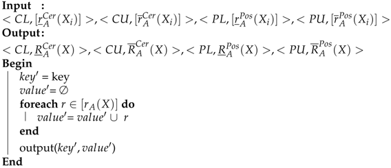
For each X i X , we first compute X C e r = X i , and X P o s = X i U d = following Equation (2). We then use X C e r to compute r ̲ A C e r ( X i ) , r ¯ A C e r ( X i ) following Equation (4), and use X P o s to r ̲ A P o s ( X i ) , r ¯ A P o s ( X i ) following Equation (6). Note that C e r ( U / A ) and P o s ( U / A ) are results from the AP step. Our output keys are C L , C U , P L , P U , which stands for certain lower, certain upper, possible lower, and possible upper approximations, respectively. In reducers, we iterate over the list of rough approximations of X i , and aggregate them. The final result is the rough approximations of X. Note that, in our RA Reduce, we use the denotation r A ( X ) to represent r ̲ A P o s ( X i ) , r ¯ A P o s ( X i ) , r ̲ A C e r ( X i ) , and r ¯ A C e r ( X i ) .
Example 6.
(Example 5 continued) Let X = U d / d = { { x 1 , x 5 , x 7 } , { x 2 } , { x 3 , x 6 } , { x 8 } } , and U d = = { x 4 } . The output of RA Map:
Map1: ( X i = X C e r = { x 1 , x 5 , x 7 } , X P o s = { x 1 , x 4 , x 5 , x 7 } )
< C L , r ̲ A C e r ( X i ) = > , < C U , r ¯ A C e r ( X i ) = { { x 5 } , { x 1 , x 4 } } > , < P L , r ̲ A P o s ( X i ) = { { x 5 } , { x 7 } , { x 1 , x 4 , x 7 } } > , < P U , r ¯ A P o s ( X i ) = { { x 7 } , { x 2 , x 5 } , { x 3 , x 6 , x 7 } , { x 1 , x 4 , x 7 } } > .
Map2: ( X i = X C e r = { x 2 } , X P o s = { x 2 , x 4 } )
< C L , r ̲ A C e r ( X i ) = > , < C U , r ¯ A C e r ( X i ) = > , < P L , r ̲ A P o s ( X i ) = { { x 2 } , { x 4 } } > , < P U , r ¯ A P o s ( X i ) = { { x 2 } , { x 2 , x 8 } , { x 2 , x 5 } , { x 2 , x 3 , x 6 } , { x 1 , x 4 , x 7 } } > .
Map3: ( X i = X C e r = { x 3 , x 6 } , X P o s = { x 3 , x 4 , x 6 } )
< C L , r ̲ A C e r ( X i ) = > , < C U , r ¯ A C e r ( X i ) = > , < P L , r ̲ A P o s ( X i ) = { { x 3 , x 6 } , { x 4 } } > , < P U , r ¯ A P o s ( X i ) = { { x 3 , x 6 } , { x 2 , x 3 , x 6 } , { x 3 , x 6 , x 7 } , { x 1 , x 4 , x 7 } } > .
Map4: ( X i = X C e r = { x 8 } , X P o s = { x 4 , x 8 } )
< C L , r ̲ A C e r ( X i ) = > , < C U , r ¯ A C e r ( X i ) = { x 8 } > , < P L , r ̲ A P o s ( X i ) = { { x 8 } , { x 4 } } > , < P U , r ¯ A P o s ( X i ) = { { x 2 , x 8 } , { x 1 , x 4 , x 7 } } > .
Map5: ( X P o s = { x 4 } ) < P L , r ̲ A P o s ( X i ) = { x 4 } > , < P U , r ¯ A P o s ( X i ) = { x 1 , x 4 , x 7 } > .
The output of RS-Reduce:
< C L , R ̲ A C e r ( X ) = > , < C U , R ¯ A C e r ( X ) = { { x 8 } , { x 5 } , { x 1 , x 4 } } > ,
< P L , R ̲ A P o s ( X ) = { { x 2 } , { x 5 } , { x 7 } , { x 8 } , { x 3 , x 6 } , { x 1 , x 4 , x 7 } } > ,
< P U , R ¯ A P o s ( X ) = { { x 2 } , { x 7 } , { x 2 , x 5 } , { x 2 , x 8 } , { x 3 , x 6 } , { x 2 , x 3 , x 6 } , { x 3 , x 6 , x 7 } , { x 1 , x 4 , x 7 } } > .
These results coincide with those in Example 1.
Proposition 6.
The twofold rough approximations of the target set X produced by the sequential and parallel algorithms are the same.
Proof. 
From Propositions 1–5, we see that our proposed parallel algorithms generate the same results at each corresponding step of the sequentiaL Algorithm 1. This ensures that our proposed algorithms give the final rough approximations as those from the sequential algorithm. ☐
Proposition 6 verifies the correctness of our proposed parallel approach since it produces the same results as the sequential approach. Our approach can generalize well not only for IDS but also for IIS. Since IIS is the special case of IDS when the decision attribute has no missing data, Algorithm 8 can change a little to be adapted for IIS. In the case of IIS, U d = is empty, so X C e r coincides with X P o s . Other algorithms can be used in IIS without modification. Thus, our proposed approach can be used as a validation tool for other current approaches that deal with just the missing data in condition attributes of big datasets.

5.3. Evaluation Test

In this part, we will evaluate the performance of sequential and parallel algorithms on different databases. The sequential algorithm is run on a computer with Intel Core i7 7700K (eight cores, each core has a clock frequency of 4.2 Ghz), and 16 GB main memory. We run the parallel algorithm on a cluster with five nodes, one is a master, and four slaves, each slave runs Intel Core i5 650 (four cores, each has a clock frequency of 3.2 Ghz) and has 8 GB main memory. We do experiments in Ubuntu 17.10, JDK 9.0.1, and Hadoop 2.9.0 environments. We only evaluate the efficiency of the algorithms in terms of execution time, not its accuracy since our parallel algorithm produces the same results as those of the sequential algorithm.
We conduct experiments on commonly used machine learning datasets, KDDCup99 from the UCI Machine Learning repository [74]. The dataset has approximately 5 million records, and each record consists of one decision attribute and 41 condition attributes. Since our parallel algorithms deal with categorical attributes, all 35 numeric attributes are discretized first. Furthermore, we create missing data on both condition and decision attributes at the one percent rate and the dataset is renamed Kdd100. To test efficiency of the proposed method with different sizes of datasets, we divide the Kdd100 dataset into smaller datasets. Datasets are named based on the percentage, e.g., Kdd10 stands for 10 percent of original dataset, and so on (Table 6).
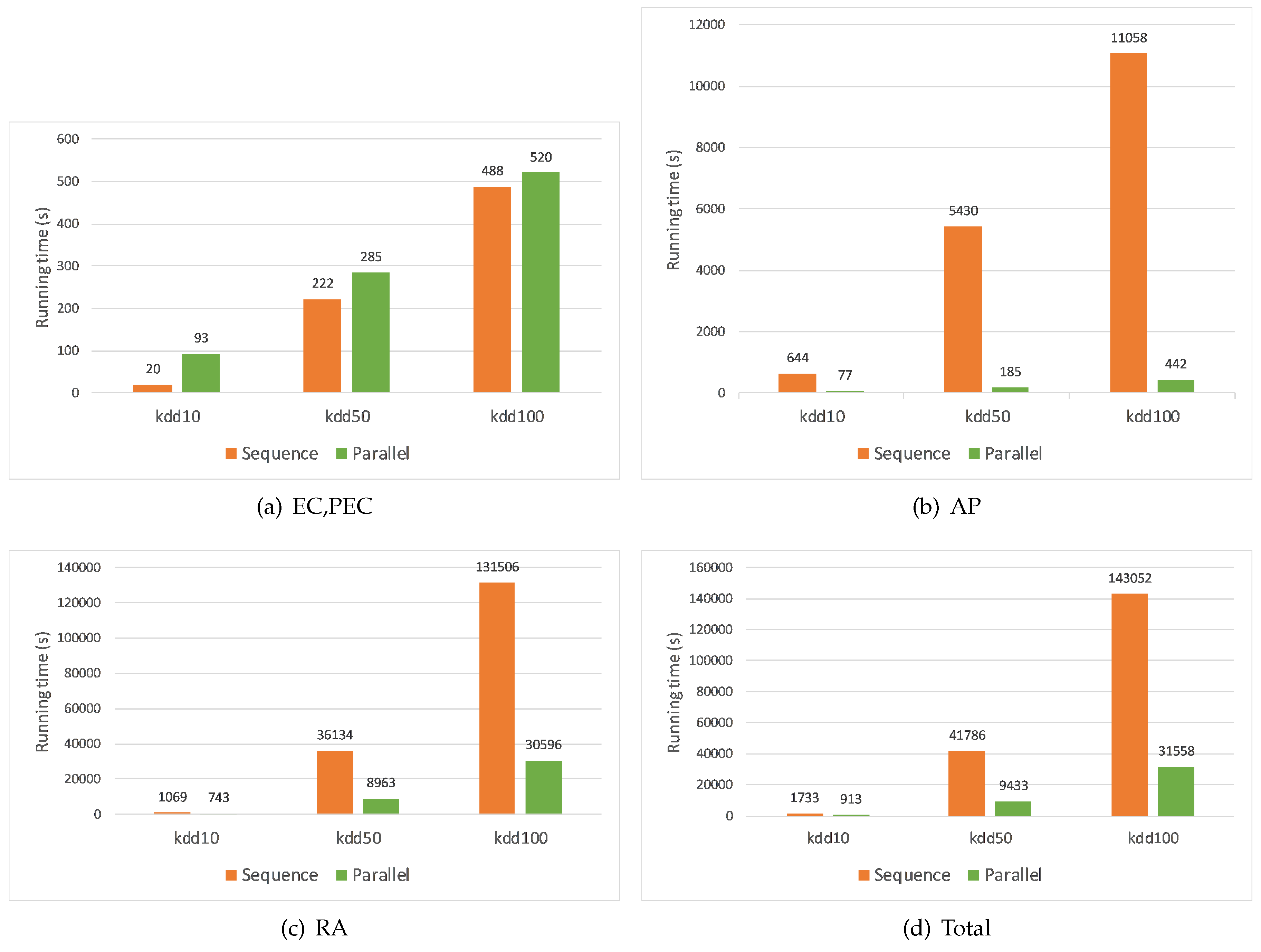
Figure 2 shows the comparison of execution time between the sequential and parallel algorithms. We compare execution time by each step of the Algorithm 1 and the corresponding step of the parallel algorithms. When performing Step 2 of the sequential algorithm, we met the insufficient memory error if we aggregated more than eight condition attributes. Hence, we decided to aggregate only 8 out of 41 condition attributes to be able to measure its execution time. Our data and source code can be found here [75]. From the results of our experiments, we can draw some conclusions:
  • Execution time increases when the volume of data increases in both sequential and parallel algorithms.
  • The most intensive step is RA step, and the least intensive step is EC, PEC step. The AP step takes less time than the RA step in our experiments because we aggregate very few condition attributes. The more attributes we aggregate, the more time the AP step will take.
  • In AP and RA steps, the parallel algorithms outperform the sequential algorithm. To the dataset Kdd100, the former performs 25 times faster than the latter at the AP step, and four times faster at the RA step, respectively. This is important since these are the most intensive computational steps. For the EC, PEC step, the parallel algorithm costs more time. This is because we divide this step into two separate MapReduce jobs: EC and PEC. Since each job requires a certain time to start up its mappers and reducers, the time consumed by both jobs becomes larger than the one of the sequential algorithm, especially when the input data is small. Notice that the time difference becomes smaller when the input data is larger (63 s in case of Kdd50, and 32 s in case of Kdd100). It is intuitive that the parallel algorithm is more efficient if we input larger datasets. In addition, since this step costs the least amount of time, it will not impact the total execution time of both algorithms.
  • As the size of the input data increases, the parallel algorithm outperforms the sequential algorithm. We can verify this through the total execution time. The parallel algorithm is around four times less than the sequential algorithm in datasets Kdd50 and Kdd100. This proves the efficiency of our proposed parallel algorithm.
As we can observe, our proposed parallel is more efficient in terms of computation time than the sequential method. It is worth mentioning that the sequential algorithm was implemented on a machine with a faster CPU with more memory while our parallel algorithm was implemented on a cluster of less powerful machines. We could have gotten better results if we implemented the sequential algorithm on the same configuration used for the parallel algorithm. However, we could not due to the insufficient memory error during the implementation of the sequential method.
With the limit on the number of machines available, we could not arrange a bigger cluster with more nodes so that more rigorous experiments and larger datasets can be tested. We aim to do this in the future. In addition, more optimization settings such as compressed types, data blocksizes, etc should be more carefully considered. Changing these settings may affect the performance of our parallel algorithm.

6. Conclusions

In this emerging era of big data, a large-scale information system with both conditions missing and decision values are normally seen in practice. Such information systems are difficult to cope with, not only because of the incomplete information they contain, but also because they are large in size. In this paper, we have successfully extended the method of twofold rough approximations for such massive, incomplete information systems. In addition, computing rough approximations by the sequential approach is very slow; thus, different MapReduce-based parallel algorithms are proposed to accelerate the computation. Experimental results demonstrate that our proposed parallel methods outperform the sequential method. Since computing rough approximations plays a key role in rule extraction and features reduction when utilizing rough set-based methods, our future work is to further investigate rules extraction and features reduction from such massive, incomplete information systems based on rough sets.

Author Contributions

Conceptualization, K.Y.; Formal analysis, M.U.; Methodology, T.C. and D.V.N.; Resources, T.C. and I.S.; Software, T.C. and I.S.; Supervision, K.Y. and D.V.N.; Writing-Review and Editing, T.C.

Funding

This research received no external funding.

Conflicts of Interest

The authors declare no conflict of interest.

References

  1. Pawlak, Z. Rough sets. In International Journal of Computer and Information Sciences; Kluwer Acad.: South Holland, The Netherlands, 1982; Volume 11, pp. 341–356. [Google Scholar]
  2. Pawlak, Z. Rough Sets. In Theoretical Aspects of Reasoning Data; Kluwer Acad.: South Holland, The Netherlands, 1991. [Google Scholar]
  3. Zhao, H.; Wang, P.; Hu, Q. Cost-sensitive feature selection based on adaptive neighborhood granularity with multi-level confidence. Inf. Sci. 2016, 366, 134–149. [Google Scholar] [CrossRef]
  4. Ju, H.; Li, H.; Yang, X.; Zhou, X.; Huang, B. Cost-sensitive rough set: A multi-granulation approach. Knowl. Based Syst. 2017, 123, 137–153. [Google Scholar] [CrossRef]
  5. Liang, J.; Wang, F.; Dang, C.; Qian, Y. A Group Incremental Approach to Feature Selection Applying Rough Set Technique. IEEE Trans. Knowl. Data Eng. 2014, 26, 294–308. [Google Scholar] [CrossRef]
  6. Yao, Y.; Zhang, X. Class-specific attribute reducts in rough set theory. Inf. Sci. 2017, 418–419, 601–618. [Google Scholar] [CrossRef]
  7. Roy, J.; Adhikary, K.; Kar, S.; Pamucar, D. A rough strength relational DEMATEL model for analysing the key success factors of hospital service quality. In Decision Making: Applications in Management and Engineering; Electrocore: Bernards Township, NJ, USA, 2018. [Google Scholar]
  8. Tay, F.E.; Shen, L. Economic and financial prediction using rough sets model. Eur. J. Oper. Res. 2002, 141, 641–659. [Google Scholar] [CrossRef] [Green Version]
  9. Goh, C.; Law, R. Incorporating the rough sets theory into travel demand analysis. Tour. Manag. 2003, 24, 511–517. [Google Scholar] [CrossRef]
  10. Ma, T.; Zhou, J.; Tang, M.; Tian, Y.; Al-Dhelaan, A.; Al-Rodhaan, M.; Lee, S. Social network and tag sources based augmenting collaborative recommender system. IEICE Trans. Inf. Syst. 2015, E98D, 902–910. [Google Scholar] [CrossRef]
  11. Karavidic, Z.; Projovic, D. A multi-criteria decision-making (MCDM) model in the security forces operations based on rough sets. In Decision Making: Applications in Management and Engineering; Electrocore: Bernards Township, NJ, USA, 2018; Volume 1, pp. 97–120. [Google Scholar]
  12. Swiniarski, R.; Skowron, A. Rough set methods in feature selection and recognition. Pattern Recognit. Lett. 2003, 24, 833–849. [Google Scholar] [CrossRef] [Green Version]
  13. Wei, J.M.; Wang, S.Q.; Yuan, X.J. Ensemble rough hypercuboid approach for classifying cancers. IEEE Trans. Knowl. Data Eng. 2010, 22, 381–391. [Google Scholar] [CrossRef]
  14. Yao, Y.; Zhou, B. Two Bayesian approaches to rough sets. Eur. J. Oper. Res. 2016, 251, 904–917. [Google Scholar] [CrossRef]
  15. Yao, Y. Three-Way Decisions and Cognitive Computing. Cognit. Comput. 2016, 8, 543–554. [Google Scholar] [CrossRef]
  16. Yao, Y. The two sides of the theory of rough sets. Knowl. Based Syst. 2015, 80, 67–77. [Google Scholar] [CrossRef]
  17. Liu, D.; Li, T.; Liang, D. Incorporating logistic regression to decision-theoretic rough sets for classifications. Int. J. Approx. Reason. 2014, 55, 197–210. [Google Scholar] [CrossRef]
  18. Xu, J.; Miao, D.; Zhang, Y.; Zhang, Z. A three-way decisions model with probabilistic rough sets for stream computing. Int. J. Approx. Reason. 2017, 88, 1–22. [Google Scholar] [CrossRef]
  19. Li, H.; Li, D.; Zhai, Y.; Wang, S.; Zhang, J. A novel attribute reduction approach for multi-label data based on rough set theory. Inf. Sci. 2016, 367, 827–847. [Google Scholar] [CrossRef]
  20. Zheng, Y.; Jeon, B.; Xu, D.; Wu, Q.J.; Zhang, H. Image Segmentation by Generalized Hierarchical Fuzzy C-means Algorithm. J. Intell. Fuzzy Syst. 2015, 28, 961–973. [Google Scholar]
  21. Lin, T. Data mining and machine oriented modeling: A granular computing approach. Appl. Intell. 2000, 13, 113–124. [Google Scholar] [CrossRef]
  22. Cao, T.; Yamada, K.; Unehara, M.; Suzuki, I.; Nguyen, D.V. Semi-supervised based rough set to handle missing decision data. In Proceedings of the 2016 IEEE International Conference on Fuzzy Systems, FUZZ-IEEE, Vancouver, BC, Canada, 24–29 July 2016; pp. 1948–1954. [Google Scholar]
  23. Cao, T.; Yamada, K.; Unehara, M.; Suzuki, I.; Nguyen, D.V. Rough Set Model in Incomplete Decision Systems. J. Adv. Comput. Intell. Intell. Inform. 2017, 21, 1221–1231. [Google Scholar] [CrossRef]
  24. Li, Y.; Jin, Y.; Sun, X. Incremental method of updating approximations in DRSA under variations of multiple objects. Int. J. Mach. Learn. Cybern. 2018, 9, 295–308. [Google Scholar] [CrossRef]
  25. Zhang, J.; Li, T.; Ruan, D.; Gao, Z.; Zhao, C. A parallel method for computing rough set approximations. Inf. Sci. 2012, 194, 209–223. [Google Scholar] [CrossRef]
  26. Zhang, J.; Wong, J.S.; Li, T.; Pan, Y. A comparison of parallel large-scale knowledge acquisition using rough set theory on different MapReduce runtime systems. Int. J. Approx. Reason. 2014, 55, 896–907. [Google Scholar] [CrossRef]
  27. Chen, H.; Li, T.; Cai, Y.; Luo, C.; Fujita, H. Parallel attribute reduction in dominance-based neighborhood rough set. Inf. Sci. 2016, 373, 351–368. [Google Scholar] [CrossRef]
  28. Li, S.; Li, T.; Zhang, Z.; Chen, H.; Zhang, J. Parallel computing of approximations in dominance-based rough sets approach. Knowl. Based Syst. 2015, 87, 102–111. [Google Scholar] [CrossRef]
  29. Qian, J.; Miao, D.; Zhang, Z.; Yue, X. Parallel attribute reduction algorithms using MapReduce. Inf. Sci. 2014, 279, 671–690. [Google Scholar] [CrossRef]
  30. Qian, J.; Lv, P.; Yue, X.; Liu, C.; Jing, Z. Hierarchical attribute reduction algorithms for big data using MapReduce. Knowl. Based Syst. 2015, 73, 18–31. [Google Scholar] [CrossRef]
  31. Li, S.; Li, T. Incremental update of approximations in dominance-based rough sets approach under the variation of attribute values. Inf. Sci. 2015, 294, 348–361. [Google Scholar] [CrossRef]
  32. Liu, D.; Li, T.; Zhang, J. A rough set-based incremental approach for learning knowledge in dynamic incomplete information systems. Int. J. Approx. Reason. 2014, 55, 1764–1786. [Google Scholar] [CrossRef]
  33. Shu, W.; Shen, H. Incremental feature selection based on rough set in dynamic incomplete data. Pattern Recognit. 2014, 47, 3890–3906. [Google Scholar] [CrossRef]
  34. Hu, J.; Li, T.; Luo, C.; Li, S. Incremental fuzzy probabilistic rough sets over dual universes. In Proceedings of the 2015 IEEE International Conference on Fuzzy Systems (FUZZ-IEEE), Istanbul, Turkey, 2–5 August 2015; pp. 1–8. [Google Scholar]
  35. Jin, Y.; Li, Y.; He, Q. A fast positive-region reduction method based on dominance-equivalence relations. In Proceedings of the 2016 International Conference on Machine Learning and Cybernetics (ICMLC), Jeju Island, South Korea, 10–13 July 2016; Volume 1, pp. 152–157. [Google Scholar]
  36. Dean, J.; Ghemawat, S. MapReduce: Simplified data processing on large clusters. In Proceedings of the 6th conference on Symposium on Operating Systems Design and Implementation, San Francisco, CA, USA, 6–8 December 2004. [Google Scholar]
  37. Nakata, M.; Sakai, H. Twofold rough approximations under incomplete information. Int. J. Gen. Syst. 2013, 42, 546–571. [Google Scholar] [CrossRef]
  38. Slezak, D.; Ziarko, W. Bayesian rough set model. In Proceedings of the International Workshop on Foundation of Data Mining (FDM2002), Maebashi, Japan, 9 December 2002; pp. 131–135. [Google Scholar]
  39. Van Nguyen, D.; Yamada, K.; Unehara, M. Extended tolerance relation to define a new rough set model in incomplete information systems. Adv. Fuzzy Syst. 2013, 2013, 372091. [Google Scholar] [CrossRef]
  40. Van Nguyen, D.; Yamada, K.; Unehara, M. Rough set approach with imperfect data based on Dempster-Shafer theory. J. Adv. Comput. Intell. Intell. Inform. 2014, 18, 280–288. [Google Scholar] [CrossRef]
  41. Grzymala-Busse, J.W. On the unknown attribute values in learning from examples. In Methodologies for Intelligent Systems; Ras, Z., Zemankova, M., Eds.; Springer: Berlin, Germany, 1991; Volume 542, pp. 368–377. [Google Scholar]
  42. Grzymala-Busse, J.; Hu, M. A comparison of several approaches to missing attribute values in data mining. In Rough Sets and Current Trends in Computing; Ziarko, W., Yao, Y., Eds.; Springer: Berlin, Germany, 2001; Volume 2005, pp. 378–385. [Google Scholar]
  43. Grzymala-Busse, J. Characteristic relations for incomplete data: A generalization of the indiscernibility relation. In Proceedings of the Third International Conference on Rough Sets and Current Trends in Computing, Uppsala, Sweden, 1–5 June 2004; pp. 244–253. [Google Scholar]
  44. Grzymala-Busse, J. Three approaches to missing attribute values: A rough set perspective. In Data Mining: Foundations and Practice; Lin, T., Xie, Y., Wasilewska, A., Liau, C.J., Eds.; Springer: Berlin, Germany, 2008; Volume 118, pp. 139–152. [Google Scholar]
  45. Grzymala-Busse, J.W.; Rzasa, W. Definability and other properties of approximations for generalized indiscernibility relations. In Transactions on Rough Sets XI; Peters, J., Skowron, A., Eds.; Springer: Berlin, Germany, 2010; Volume 5946, pp. 14–39. [Google Scholar]
  46. Guan, L.; Wang, G. Generalized approximations defined by non-equivalence relations. Inf. Sci. 2012, 193, 163–179. [Google Scholar] [CrossRef]
  47. Stefanowski, J.; Tsoukias, A. On the extension of rough sets under incomplete information. In Proceedings of the New directions in rough sets, data mining and granular-soft computing, Yamaguchi, Japan, 11–19 November 1999; pp. 73–82. [Google Scholar]
  48. Stefanowski, J.; Tsoukias, A. Incomplete information tables and rough classication. Comput. Intell. 2001, 17, 545–566. [Google Scholar] [CrossRef]
  49. Katzberg, J.D.; Ziarko, W. Variable precision rough sets with asymmetric bounds. In Proceedings of the International Workshop on Rough Sets and Knowledge Discovery: Rough Sets, Fuzzy Sets and Knowledge Discovery, Banff, AB, Canada, 12–15 October 1993; Springer: London, UK, 1994; pp. 167–177. [Google Scholar]
  50. Kryszkiewicz, M. Rough set approach to incomplete information systems. Inf. Sci. 1998, 112, 39–49. [Google Scholar] [CrossRef]
  51. Kryszkiewicz, M. Rules in incomplete information systems. Inf. Sci. 1999, 113, 271–292. [Google Scholar] [CrossRef]
  52. Leung, Y.; Li, D. Maximal consistent block technique for rule acquisition in incomplete information systems. Inf. Sci. 2003, 153, 85–106. [Google Scholar] [CrossRef]
  53. Leung, Y.; Wu, W.Z..; Zhang, W.X. Knowledge acquisition in incomplete information systems: A rough set approach. Eur. J. Oper. Res. 2006, 168, 164–180. [Google Scholar] [CrossRef]
  54. Nakata, M.; Sakai, H. Handling missing values in terms of rough sets. In Proceedings of the 23rd Fuzzy System Symposium, Nayoga, Japan, 29–31 August 2007. [Google Scholar]
  55. Miao, D.; Zhao, Y.; Yao, Y.; Li, H.; Xu, F. Relative reducts in consistent and inconsistent decision tables of the Pawlak rough set model. Inf. Sci. 2009, 179, 4140–4150. [Google Scholar] [CrossRef]
  56. Slezak, D.; Ziarko, W. Variable precision bayesian rough set model. Lect. Notes Comput. Sci. 2003, 2639, 312–315. [Google Scholar]
  57. Slezak, D.; Ziarko, W. Attribute reduction in the Bayesian version of variable precision rough set model. Electron. Notes Theor. Comput. Sci. 2003, 82, 263–273. [Google Scholar]
  58. Slezak, D.; Ziarko, W. The investigation of the Bayesian rough set model. Int. J. Approx. Reason. 2005, 40, 81–91. [Google Scholar] [CrossRef]
  59. Wang, G. Extension of rough set under incomplete information systems. In Proceedings of the 2002 IEEE International Conference on Fuzzy Systems, FUZZ-IEEE’02, Honolulu, Hawaii, 12–17 May 2002; Volume 2, pp. 1098–1103. [Google Scholar]
  60. Yang, X.; Yu, D.; Yang, J.; Song, X. Difference relation-based rough set and negative rules in incomplete information system. Int. J. Uncertain. Fuzz. Knowl. Based Syst. 2009, 17, 649–665. [Google Scholar] [CrossRef]
  61. Yang, X.; Yang, J. Incomplete Information System and Rough Set Theory, 1st ed.; Springer: Berlin, Germany, 2012. [Google Scholar]
  62. Medhat, T. Prediction of missing values for decision attribute. J. Inform. Technol. Comput. Sci. 2012, 4, 58–66. [Google Scholar] [CrossRef]
  63. El-Alfy, E.S.M.; Alshammari, M.A. Towards scalable rough set based attribute subset selection for intrusion detection using parallel genetic algorithm in MapReduce. Simul. Model. Pract. Theory 2016, 64, 18–29. [Google Scholar] [CrossRef]
  64. Verma, A.; Llora, X.; Goldberg, D.E.; Campbell, R.H. Scaling Genetic Algorithms Using MapReduce. In Proceedings of the 2009 Ninth International Conference on Intelligent Systems Design and Applications, Pisa, Italy, 30 November–2 December 2009; pp. 13–18. [Google Scholar]
  65. Han, L.; Liew, C.; Van Hemert, J.; Atkinson, M. A generic parallel processing model for facilitating data mining and integration. Parallel Comput. 2011, 37, 157–171. [Google Scholar] [CrossRef]
  66. McNabb, A.W.; Monson, C.K.; Seppi, K.D. Parallel PSO using MapReduce. In Proceedings of the 2007 IEEE Congress on Evolutionary Computation, Singapore, 25–28 September 2007; pp. 7–14. [Google Scholar]
  67. Chu, C.T.; Kim, S.K.; Lin, Y.A.; Yu, Y.; Bradski, G.; Ng, A.Y.; Olukotun, K. Map-reduce for Machine Learning on Multicore. In Proceedings of the 19th International Conference on Neural Information Processing Systems, Doha, Qatar, 12–15 November 2012; MIT Press: Cambridge, MA, USA, 2006; pp. 281–288. [Google Scholar]
  68. Srinivasan, A.; Faruquie, T.A.; Joshi, S. Data and task parallelism in ILP using MapReduce. Mach. Learn. 2012, 86, 141–168. [Google Scholar] [CrossRef]
  69. Zhao, W.; Ma, H.; He, Q. Parallel K-Means Clustering Based on MapReduce. In Cloud Computing; Jaatun, M.G., Zhao, G., Rong, C., Eds.; Springer: Berlin, Germany, 2009; pp. 674–679. [Google Scholar]
  70. Zinn, D.; Bowers, S.; Kohler, S.; Ludascher, B. Parallelizing XML data-streaming workflows via MapReduce. J. Comput. Syst. Sci. 2010, 76, 447–463. [Google Scholar] [CrossRef]
  71. Li, P.; Wu, J.; Shang, L. Fast approximate attribute reduction with MapReduce. In Lecture Notes in Computer Science (Including Subseries Lecture Notes in Artificial Intelligence and Lecture Notes in Bioinformatics); Springer: Berlin, Germany, 2013; pp. 271–278. [Google Scholar]
  72. Zhang, J.; Wong, J.S.; Pan, Y.; Li, T. A Parallel Matrix-Based Method for Computing Approximations in Incomplete Information Systems. IEEE Trans. Knowl. Data Eng. 2015, 27, 326–339. [Google Scholar] [CrossRef]
  73. Yuan, J.; Chen, M.; Jiang, T.; Li, T. Complete tolerance relation based parallel filling for incomplete energy big data. Knowl. Based Syst. 2017, 132, 215–225. [Google Scholar] [CrossRef]
  74. Data, K.C. KDD Cup 1999 Data. Available online: http://kdd.ics.uci.edu/databases/kddcup99/kddcup99.html (accessed on 18 August 2018).
  75. Sourcecode. Available online: https://github.com/KennyThinh/ParallelComputationTwoFoldRS (accessed on 18 August 2018).
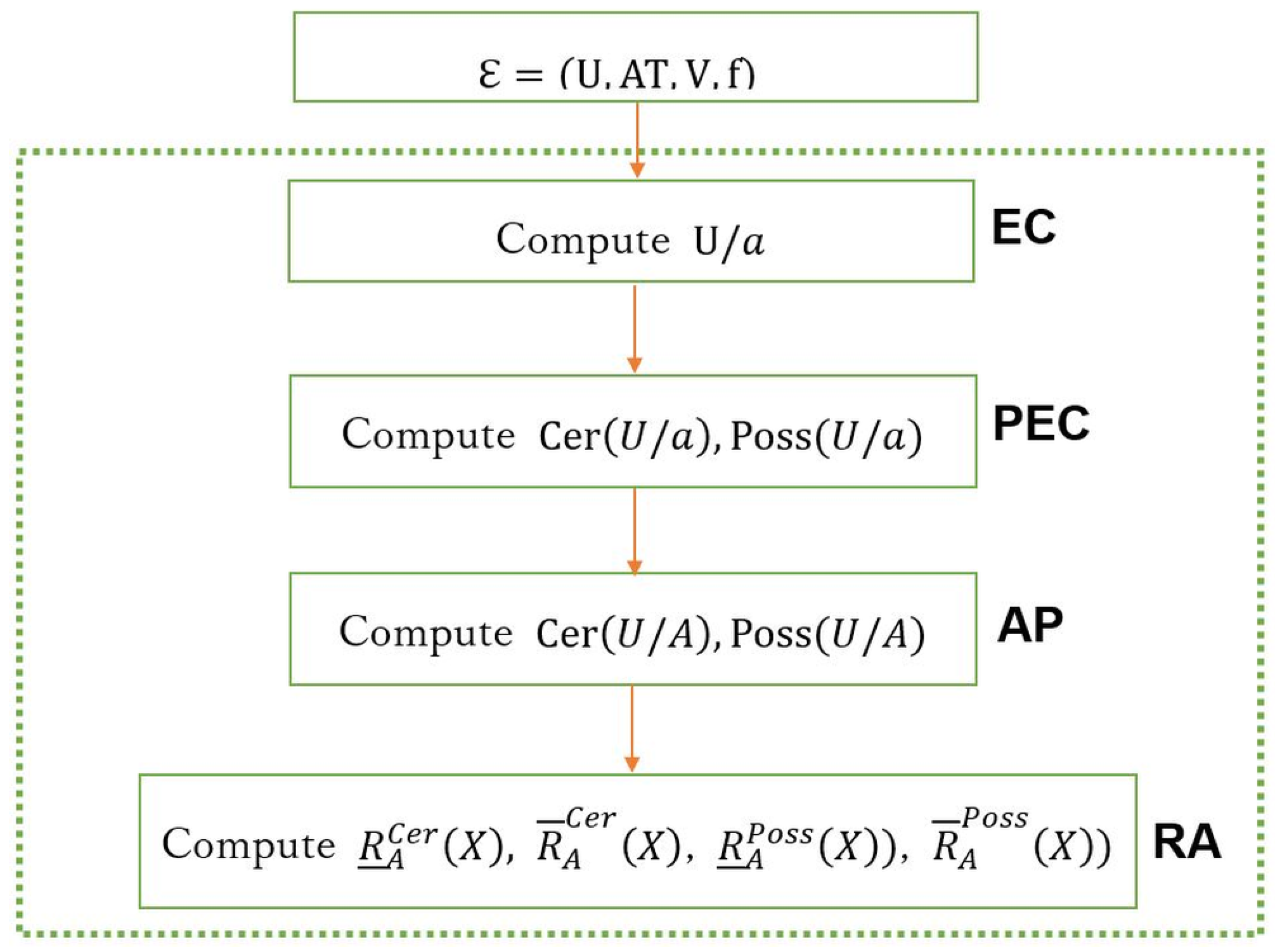
Figure 1. MapReduce-based parallel computation.
Computers 07 00044 g001
Figure 2. Compare execution time of each step between sequential and parallel algorithms: (a) Step 1 of the sequential algorithm and EC, PEC steps of the parallel algorithm, (b) Step 2 of the sequential algorithm and AP step of the parallel algorithm, (c) Steps 3,4 of the sequential algorithm and RA step of the parallel algorithm, and (d) total steps of the sequential and parallel algorithms.
Computers 07 00044 g002
Table 1. An example of IDS.
a 1 a 2 d
x 1 120
x 2 *11
x 3 2*2
x 4 12*
x 5 110
x 6 2*2
x 7 *20
x 8 313
Table 2. Calculate C e r ( U / a ) and P o s ( U / a ) .
a a 1 a 2
U a / a c { x 1 , x 4 , x 5 } , { x 3 , x 6 } , { x 8 } { x 2 , x 5 , x 8 } , { x 1 , x 4 , x 7 }
U a = { x 2 , x 7 } { x 3 , x 6 }
C e r ( U / a ) c { x 1 , x 4 , x 5 } , { x 3 , x 6 } , { x 8 } , { x 2 , x 5 , x 8 } , { x 1 , x 4 , x 7 } ,
P o s ( U / a ) c { x 2 , x 7 } , { x 1 , x 2 , x 4 , x 5 , x 7 } , { x 2 , x 3 , x 6 , x 7 } , { x 2 , x 7 , x 8 } c { x 3 , x 6 } , { x 2 , x 3 , x 5 , x 6 , x 8 } , { x 1 , x 3 , x 4 , x 6 , x 7 }
Table 3. Calculate r ̲ A C e r ( x ) and r ¯ A C e r ( x ) .
x X C e r r ̲ A C e r ( x ) r ¯ A C e r ( x )
{ x 1 , x 5 , x 7 } { x 5 } , { x 1 , x 4 }
{ x 2 }
{ x 3 , x 6 }
{ x 8 } { x 8 }
Table 4. Calculate r ̲ A P o s ( x ) and r ¯ A P o s ( x ) .
x X P o s r ̲ A P o s ( x ) r ¯ A P o s ( x )
{ x 1 , x 4 , x 5 , x 7 } { x 5 } , { x 7 } , { x 1 , x 4 , x 7 } { x 7 } , { x 2 , x 5 } , { x 3 , x 6 , x 7 } , { x 1 , x 4 , x 7 }
{ x 2 , x 4 } { x 2 } , { x 4 } { x 2 } , { x 2 , x 8 } , { x 2 , x 5 } , { x 2 , x 3 , x 6 } , { x 1 , x 4 , x 7 }
{ x 3 , x 4 , x 6 } { x 3 , x 6 } , { x 4 } c { x 3 , x 6 } , { x 2 , x 3 , x 6 } , { x 3 , x 6 , x 7 } , { x 1 , x 4 , x 7 }
{ x 4 , x 8 } { x 8 } , { x 4 } { x 2 , x 8 } , { x 1 , x 4 , x 7 }
{ x 4 } { x 4 } { x 1 , x 4 , x 7 }
Table 5. Sub-IDS.
Table 5. Sub-IDS.
U 1 a 1 a 2 d U 2 a 1 a 2 d
x 1 120 x 5 110
x 2 *11 x 6 2*2
x 3 2*2 x 7 *21
x 4 12* x 8 313
Table 6. A description of datasets.
RecordsSize (MB)
Kdd10489,84444
Kdd502,449,217219
Kdd104,898,431402