Article

Semi-Automatic Image Labelling Using Depth Information

by
Mostafa Pordel
1,2,* and
Thomas Hellström
1
1
Department of Computing Science, Umeå University, Umeå, SE-901 87, Sweden
2
Australian National University, Acton ACT 2601, Australia
*
Author to whom correspondence should be addressed.
Computers 2015, 4(2), 142-154; https://doi.org/10.3390/computers4020142
Submission received: 11 June 2013 / Accepted: 14 April 2015 / Published: 6 May 2015

Abstract

:
Image labeling tools help to extract objects within images to be used as ground truth for learning and testing in object detection processes. The inputs for such tools are usually RGB images. However with new widely available low-cost sensors like Microsoft Kinect it is possible to use depth images in addition to RGB images. Despite many existing powerful tools for image labeling, there is a need for RGB-depth adapted tools. We present a new interactive labeling tool that partially automates image labeling, with two major contributions. First, the method extends the concept of image segmentation from RGB to RGB-depth using Fuzzy C-Means clustering, connected component labeling and superpixels, and generates bounding pixels to extract the desired objects. Second, it minimizes the interaction time needed for object extraction by doing an efficient segmentation in RGB-depth space. Very few clicks are needed for the entire procedure compared to existing, tools. When the desired object is the closest object to the camera, which is often the case in robotics applications, no clicks at all are required to accurately extract the object.

1. Introduction

Object detection methods need a set of labeled images for training and testing. Image labeling tools identify regions of interest, automatically or in interaction with the user who then assigns labels, i.e., object types, to them. Boundary localization of desired objects in images and videos remains a fundamental and classical problem in image segmentation [1]. Objects usually consist of several non-similar segments and are very hard to extract automatically or manually. In order to label a desired object in an image, existing tools usually let the user draw a bounding box around the object and label it with the object type.
Figure 1 shows how bounding boxes are used to extract trees, a stone, a human, and a bush in four images. The use of bounding boxes is often the simplest and fastest technique for image labeling, mainly because it avoids many details in the extracted area. In addition to the object of interest, it also includes parts of the background. Many learning algorithms may confuse the background with the object in the learning process. An alternative, or complement, to bounding boxes is bounding pixels or bounding curves that only enclose the object of interest [2,3]. However, manually specifying such a bounding curve is very challenging and time consuming. Therefore, a tool that partly automates this process would be highly valuable and could be designed as follows. First, a bounding box is manually constructed around the object that covers a region R. Then, a curve C , initially coinciding with the bounding box, is gradually modified towards the boundary δR of object R. Ideally, the entire object is extracted using only this single curve. However, some background Rc may still be inside C , and some part of R may also be outside C . For the simplest case, and for the sake of formulating the problem, we assume that the object and background form a binary image. A perfect object extraction is achieved if | ( i = 1 n I o i ) / n ( k = 1 m I i k ) / m | is maximized, where Io1, …, Ion are the intensities for the n pixels outside C , and Ii1, …, Iim are the intensities for the m pixels inside C . The maxima is achieved when C = δ R. This means that the best bounding maximizes the difference between average pixel intensities outside and inside the curve. Equally, the best bounding curve C (or bounding pixels) minimizes the following energy equation [3]:
E = 1 / 2 ( ( j = 1 n I o j ) / n ( k = 1 m I i k ) / m ) 2
Minimizing Equation (1) over all possible curves C is an NP problem [4], which is the reason why many researcher estimate the optimal solution with techniques like eigenvector-based methods [5], graph cuts [4,6], active contour [7], curve evolution [2], or other optimization and AI techniques.
In this paper we present a framework for image labeling that compute local minima of Equation (1) by a three steps algorithm that divides the extraction process into an offline mode that does most of the computations, and an online mode that executes very fast but interacts with users. A database with more than 650 images from forest environment has been collected using a Microsoft Kinect camera. The objects to be detected are categorized as bush, tree, stone and human as exemplified in Figure 1. A tool denoted ODAR (Object Detection for Agricultural Robots) has been developed to collect and label images and for each image output a set of bounding pixels C that with high accuracy defines the area R where an object is located. The remaining of this paper is organized as the following: Section 2 describes related research in image segmentation and image labeling. Section 3 describes our 3 steps method for image labeling. Fuzzy C-Means clustering is executed off-line to provide initial segments and combines RGB and depth images as explained in Section 4. Section 5 shows how the user may manually correct and edit the extracted area. Conclusions and suggestions for future work are presented in the last Section of this paper.

2. Related Work

We have evaluated several state-of-the-art techniques for image segmentation and image labeling to understand the limitations and find better solutions. Some of these techniques are presented in this section together with experimental results. Additional comparisons are presented in Section 6. There are many tools and algorithms for 2D and 3D image labeling. However, to the best of authors’ knowledge, there is no fast enough interactive tool for labeling RGB-depth images. Two of the most notable tools for image labeling are ITK-SNAP for 3D medical images [8] and LabelMe for 2D images [9]. ITK-SNAP provides manual labeling of objects by letting user to draw a polygon around an object. It also provides automated labeling using a snake algorithm for segmentation, as discussed later in this section. Polygons require many clicks from user to complete a non-efficient labeling mainly because lines are not fitted correctly to the borders of the extracted area. The automated snake algorithm is slow and also does not work well for some images, as discussed in later in this section. LabelMe is an online tool that lets the users manually draw polygons around objects, similar to ITK-SNAP. It is possible to store images online or share them with other users that are registered in LabelMe. However, functionality for automated or semi-automated labeling is missing.
Existing algorithms for image labeling can be categorized in two main groups. In bottom-up algorithms small image segments are merged together to generate bigger segments that define the desired objects. These algorithms use color, depth (if available) and appearance, e.g. edge information, to estimate borders of each segment. Image segmentation for RGB images has been studied for a long time. As a clustering problem, it can be approached with a wide range of clustering and classification algorithms like k-means [10] and K-Nearest Neighbor (KNN) [11]. Section 4 shows how we incorporate one of these techniques in our solution.
In top-down algorithms, generic or class-specific object models or contour detectors are used to extract objects within the image. The result is usually not very accurate and may need manual corrections by a human user. A major drawback with top-down algorithms is that labeled images typically are needed to create the models. Furthermore, in many cases models are not accurate enough, have high computational cost and have to be manually corrected. Generic object detection methods do not perform well for many applications, and object-specific solutions are not generally applicable. Also, the computational cost increases exponentially with the number of objects that are needed be labeled in an image. Among generic solutions, existing algorithms based on active contours are costly and usually need more than 10 s with an Intel core i5 3GH CPU to process an image with 480×640 pixels and do not perform well for image labeling. We have tried several of these algorithms and the results are shown in Figures 24 and are described later in this Section. The approach in [12] is to use a sliding window technique, and measure how likely it is that a window includes an object in general. The authors use four different image cues measuring object characteristics such as saliency [13], color contrast, edge density and superpixel straddling. Although [12] represents state of the art in object detection on the PASCAL VOC (Visual Object Classes) 07 database [14] for 2D images, the presented method does not provide bounding pixels but bounding boxes. Furthermore, as a generic method, it does not perform very well (with an average precision of about 20 percent) for all 20 objects in the VOC database. Other top-down algorithms are based on curve evolution [3]. Curve evolution based algorithms start with a curve equal to a bounding box as the initial solution to extract the objects [3]. In a series of iterations, new curves that gradually decrease the energy function in Equation (1) are computed. The algorithm stops when the improvement is less than a defined limit. The resulting curve may not be the optimal solution but is usually much better than the initial solution, and is found much faster than the optimal solution. Still, computation time and also accuracy are serious drawbacks with curve evolution based algorithms. Curve evolution is often coupled with local and regional features to enhance the evolution process and find better solutions. [15] use regional information to overcome problems caused by intensity inhomogeneities. Figures 2 and 3 show results of two of our experiments with a state-of-the-art algorithm developed by [15]. It takes about 24 s with an Intel core i5 3GH CPU to run the algorithm on one RGB and one depth image with a resolution of 480×640 pixels. As shown in the figures, the performance is fairly weak for challenging outdoor applications where it is hard to separate background from foreground.
Another popular techniques, presented in [4], is based on graph cuts that segment an RGB image in less than one second with an Intel core i5 3GHZ CPU for Microsoft Kinect images with a resolution of 480×640 pixels. Figure 4 shows the results of our tests of the algorithm. For many of our database images similar to the image of a stone on ground in Figure 4, the algorithm does not produce segments that can be used for image labeling. The authors of [16] describe object extraction with a tool inspired by the “Magic Wand” function in Adobe Photoshop, that receives user specified regions called “trimaps” to extract objects within images and videos. The main limitation of their method is that objects may be similar to background in color space. Furthermore, trimaps require many clicks for object selection if the used similarity threshold is small, and otherwise noise easily corrupts the extracted object. Figure 5 illustrates the problem graphically. Part A shows a stone extracted by three clicks with a high similarity threshold. Part B shows the same stone extracted by 10 clicks with a low threshold. This example shows the tradeoff between noise and number of necessary clicks to perform the object extraction.
An object extraction algorithm based on depth information only is presented in [17]. It uses thresholding in depth images to separate foreground from background, and label only the closest object of the image. However, the extracted foreground often includes lots of noise in the bounding area as illustrated in Figure 7C. The object extraction problem becomes harder when the object is attached to other objects with continuous depth information, such as an object placed on ground.

3. New Method for Image Labelling

As illustrated in Figure 4, distinguishing boundary edges of an object from other types of edges is a major challenges in image processing [18]. Given that depth information is more sensitive to boundary edges, it should be possible to perform image segmentation with depth images using thresholding as discussed in Section 2. Obviously using both RGB and depth images has a potential to enhance segmentation compared to only using RGB. The main question is how the images should be combined. Initially we separately segmented both RGB and depth images with all state of art methods presented in Section 2, and then fused the results with operations such as intersection and union. However, the results were not convincing and none of the methods generated good segments for image labeling (see Figures 4, 5, and 8). Furthermore, the run time for segmentation of one 480×640 pixels image with a 2GHZ dual core CPU was more than 2 s, which is too much for an interactive tool.
Therefore we extended the classical algorithm Connected Component Labeling (CCL) [19] to what we denote Extended Connected Component Labeling (ECCL). CCL assigns pixels in a binary image to the same group if they are geometrically connected but ECCL merges pixels in a color or gray image with a connected group of pixels if the difference of the new entry pixels to the group’s pixels, is less than a defined threshold (or if they are similar enough). In a lot of published research, color and texture information are used to define “similarity” and “difference” between pixels or groups of pixels. Our ECCL technique uses the “similarity” concept presented in [16], but processes the segmented image rather than the original image. We execute this segmentation off-line, prior to a step with fast interactive extraction of the areas of interest. Our method comprises the following steps:
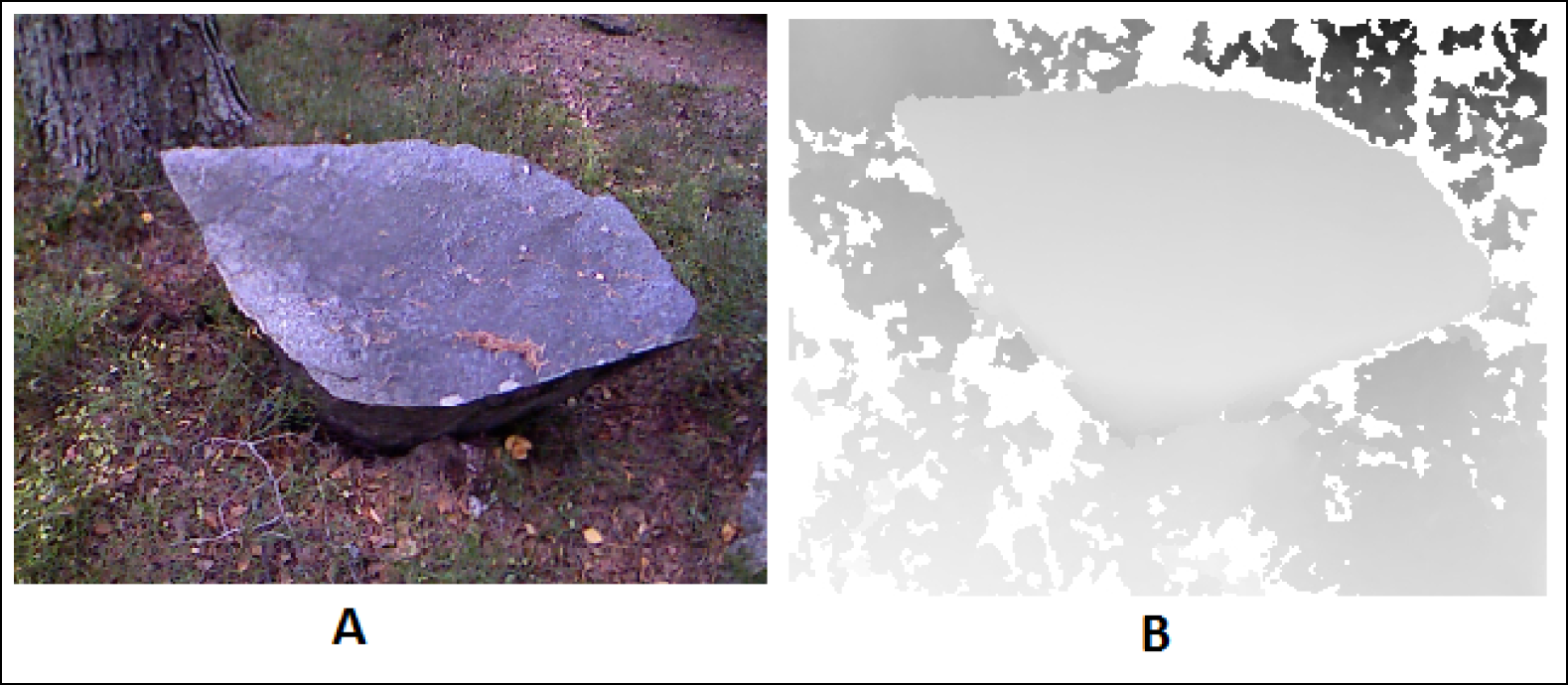
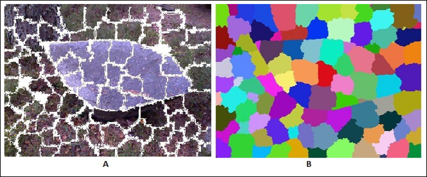
  • Segmentation of RGB and depth images
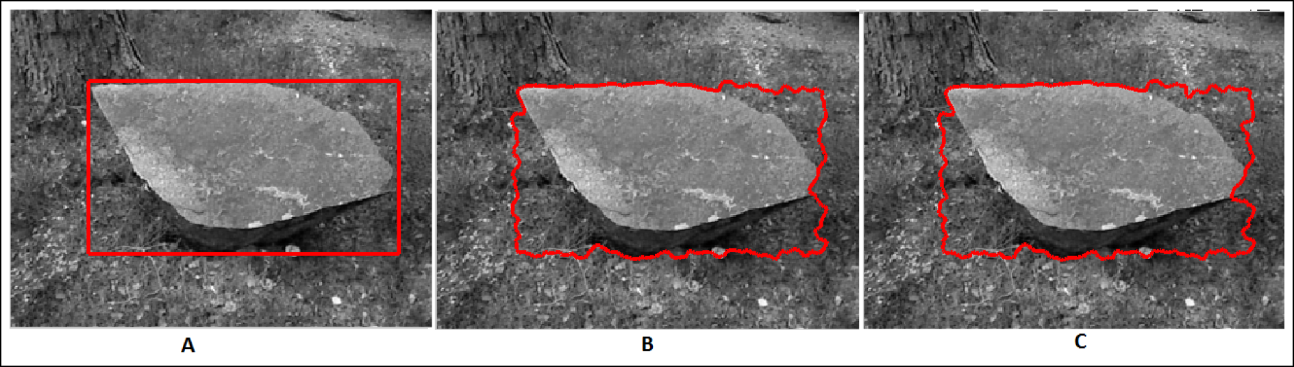
  • Interactive segmentation with ECCL
  • Interactive correction to edit the extracted area
In step 1, we use Fuzzy C-Means as described in Section 4 to fuse RGB and depth images and generate initial segments. The output does not include color or gray scale information, but multiple intensity levels that each represents a class generated from FCM. In step 2, the user may click at points on the image. ECCL uses the generated segments from step 1 and the input point(s) to extract the desired object. Since the extracted object most likely requires minor corrections, the user may edit the extracted area in the third step. This results in a very fast and efficient segmentation, with almost zero waiting time for interaction, and only a small number of required clicks.

4. Fuzzy C-Mean for Segmentation

Depth and RGB images can both contribute to the object extraction process. However, the importance of the two data sources may vary from case to case. Therefore, a flexible method to fuse information is needed. We found that the Fuzzy C-Means algorithm (FCM) for clustering [20] fits the first step of our algorithm very well. The general idea is to perform segmentation by clustering image data in feature space. The method can be seen as a generalization of thresholding in which fixed values are often used to define which pixels belong to objects and background respectively. By using a clustering algorithm, threshold values are set automatically, and the method is also directly applicable to images with several object types. FCM has previously been used for segmentation purposes, e.g. in [2124]. In our case, combinations of R, G, B, depth, and gray scale are input as features vectors to the FCM algorithm.
Let D = d1, d2, …, dn be the input data where di is a feature vector. The FCM algorithm computes a set of cluster centers C = cc1, …, ccc by minimizing the following equation:
E { D , C } = i = 1 n j = 1 c ( m i j ) w | d i c c j |
where each di has a membership degree of mij to cluster j, and w is a weighting exponent for the membership function. The initial membership values are set randomly. In each iteration, new memberships values mij and cluster centers cci are computed. The iterations stops when the changes in mij are smaller than a pre-set limit. This can be shown to correspond to a local minima for E{D,C}.
Two types of feature vectors have been evaluated. The Graydepth feature vector contains a gray scale value computed from RGB data, and depth data. The RGBdepth feature vector contains R, G, B and depth data. Figure 9 shows the result of FCM clustering to four clusters. Parts (A) and (B) show results for the Graydepth and RGBdepth feature vectors respectively. The latter feature vector leads to better segmentation, probably because of stronger dependence on depth data in the shorter feature vector, and to twice as fast algorithm since the number of features is half as many. By using FCM, initial segments are provided for next step in our labeling algorithm, as described in Section 3. Furthermore, depth and RGB images are fused such that methods like union or intersection for fusing separate segments at higher levels are not necessary.
There are two main concerns with FCM for our image labeling algorithm. First, the number of clusters has to be set in advance. Second, the memberships degrees mij are initialized to random values. This normally leads to different generated clusters, and also to different execution times, even if the user provides the same extraction points. The randomness also makes it harder to evaluate results of tests. One solution is to replace the random membership initialization with uniform membership. In practice randomness is not a problem since the user normally only labels objects once, if they are satisfied with the given solution. If not, they may run the algorithm again to get alternative solutions thanks to the random initialization.
About the first problem, if we increase the number of clusters (initial segments), the FCM algorithm will take longer time to execute. Also, the user needs to click more in step 2 of the algorithm to extract the object. On the other hand, if we decrease the number of clusters, the user needs to click more in step 3 to correct (most often to remove some part of) the extracted area. Based on our experience, between 4 and 6 clusters is suitable for most cases.

5. Segmentation Correction

Currently, practically working tools for image labeling require human interaction for verification and correction of suggested solutions. An ideal tool should minimize the number of clicks rather than offering a fully automatic process. Given an initial segmentation, the tool should allow the user to select and deselect parts of the image. Interaction at pixel level is almost impossible since individual pixels may not be visible or easily selectable. One approach is to allow the user to select and deselect smaller segments by drawing lines or polygons. This requires a line fitting algorithm, similar to curve evolution algorithms, and do not execute very fast, as described in Section 2. Another approach, which we have adopted in the proposed solution, is to let the user click at some points in the image and let the tool add or remove small segments. For this we use so called superpixels [25]. The size of each superpixel can be set depending on the application. When the user has extracted objects with the FCM and ECCL methods, superpixels may be added or removed with a few clicks to enhance the result.
Figure 8 shows superpixels for the image in Figure 6. The coloring scheme is described in [25]. The size of each superpixel vary slightly but all of them have approximately the same size. The drawback with using superpixels as primary method for object extraction is that they sometimes require many clicks to extract large objects. The optimal superpixel size depend on the specific application. The computation of superpixels may be slow, but since it can be done before image labeling, it adds no waiting time for the interactive steps in our algorithm. Figure 10 shows how an incorrect image extraction is corrected by removing several superpixels from the selected area.

6. Results

We have presented a method for labeling objects in images. It comprises steps for initial segmentation using Fuzzy C-Means (FCM) for RGB-depth features, Extended Connected Component Labeling (ECCL) for interactive basic object extraction, and finally superpixels for interactive correction. The computations of FCM and superpixels is done as pre-processing and take about 30 s for each image (with an Intel core i5 3GH CPU). The subsequent interactive ECCL algorithm runs so fast that the user do not experience any significant delay.
We evaluated the algorithm with images containing 4 types of objects; humans, bushes, trees, and stones. A database with 650 RGB and depth images were collected using the Microsoft Kinect. We compared the results with several existing algorithms, as described in Sections 2–4. Figure 11 shows some results. The first row shows the input images. The second row shows object extraction result for a single click, and the last row shows the cumulative selection coupled with low level smoothing filters.

7. Conclusions and Future Works

The proposed solution manages accurate extraction of objects using depth and RGB images, requiring only a few clicks by the user. The algorithm avoids waiting time by computing FCM and superpixels offline, while ECCL is used for user interaction in realtime. In the future, we will explore methods to feedback the user’s corrections into our algorithm such that the initial segmentation in step 1 of the algorithm gets further improved.

Acknowledgments

This work was partly funded by the European Commission (CROPS GA No. 246252).

Author Contributions

Both authors have contributed equally to the paper and approved the final manuscript.

Conflicts of Interest

The authors declare no conflict of interest

References

  1. Yhann, S.R.; Young, T.Y. Boundary localization in texture segmentation. IEEE Trans. Image Process. 1995, 4(6), 849–856. [Google Scholar]
  2. Tsai, A.; Yezzi, A.; Willsky, A. Curve evolution implementation of the Mumford-Shah functional for image segmentation, denoising, interpolation, and magnification. IEEE Trans. Image Process. 2001, 10, 1169–1186. [Google Scholar]
  3. Yezzi, A.; Tsai, A.; Willsky, A. A Fully Global Approach to Image Segmentation via Coupled Curve Evolution Equations. J. Vis. Commun. Image Represent. 2002, 13, 195–216. [Google Scholar]
  4. Felzenszwalb, P.F.; Huttenlocher, D.P. Efficient graph-based image segmentation. Int. J. Comput. Vis. 2004, 59, 167–181. [Google Scholar]
  5. Yair, W. Segmentation using eigenvectors: A unifying view. Proc. IEEE Int. Conf. Comput. Vis. 1999, 2, 975–982. [Google Scholar]
  6. Shi, J.; Malik, J. Normalized cuts and image segmentation. IEEE Trans. Pat. Anal. Mach. Intell. 2000, 22, 888–905. [Google Scholar]
  7. Vese, L.A.; Chan, T.F. A multiphase level set framework for image segmentation using the Mumford and Shah model. Int. J. Comput. Vis. 2002, 50, 271–293. [Google Scholar]
  8. Yushkevich, P.A.; Piven, J.; Heather, C.H.; Rachel, G.S.; Ho, S.; Gee, J.C.; Gerig, G. User-Guided 3D Active Contour Segmentation of Anatomical Structures: Significantly Improved Efficiency and Reliability. Neuroimage 2006, 31, 1116–1128. [Google Scholar]
  9. Russell, C.; Torralba, A.; Murphy, K.; Freeman, W. LabelMe: A Database and Web-Based Tool for Image Annotation. Int. J. Comput. Vis. 2007, 77, 157–173. [Google Scholar]
  10. Du, Q.; Gunzburger, M.; Ju, L.; Wang, X. Centroidal voronoi tessellation algorithms for image compression, segmentation, and multichannel restoration. J. Math. Imaging Vis. 2006, 24, 177–194. [Google Scholar]
  11. Chevrefils, C.; Cheriet, F.; Aubin, C.E.; Grimard, G. Texture analysis for automatic segmentation of intervertebral disks of scoliotic spines from MR images. IEEE Trans. Inf. Technol. Biomed. 2009, 13, 608–620. [Google Scholar]
  12. Alexe, B.; Deselaers, T.; Ferrari, V. What is an object? Proceedings of the IEEE Computer Society Conference on Computer Vision and Pattern Recognition, San Francisco, CA, USA, 13–18 June 2010; pp. 73–80.
  13. Hou, X.; Zhang, L. Saliency detection: A spectral residual approach, Proceedings of the IEEE Computer Society Conference on Computer Vision and Pattern Recognition, Minneapolis, MN, USA, 18–23 June 2007.
  14. Everingham, M.; van Gool, L.; Williams, C.K.I.; Winn, J.; Zisserman, A. The PASCAL Visual Object Classes Challenge 2007 (VOC 2007) Results. Available online: http://www.pascal-network.org/challenges/VOC/voc2007/workshop/index.html accessed on 16 April 2015.
  15. Li, C.; Kao, C.Y.; Gore, J.C.; Ding, Z. Minimization of region-scalable fitting energy for image segmentation. IEEE Trans. Image Process. 2008, 17, 1940–1949. [Google Scholar]
  16. Friedland, G.; Jantz, K.; Rojas, R. SIOX: Simple interactive object extraction in still images, Proceedings of the Seventh IEEE International Symposium on Multimedia, Irvine, CA, USA, 12–14 December 2005.
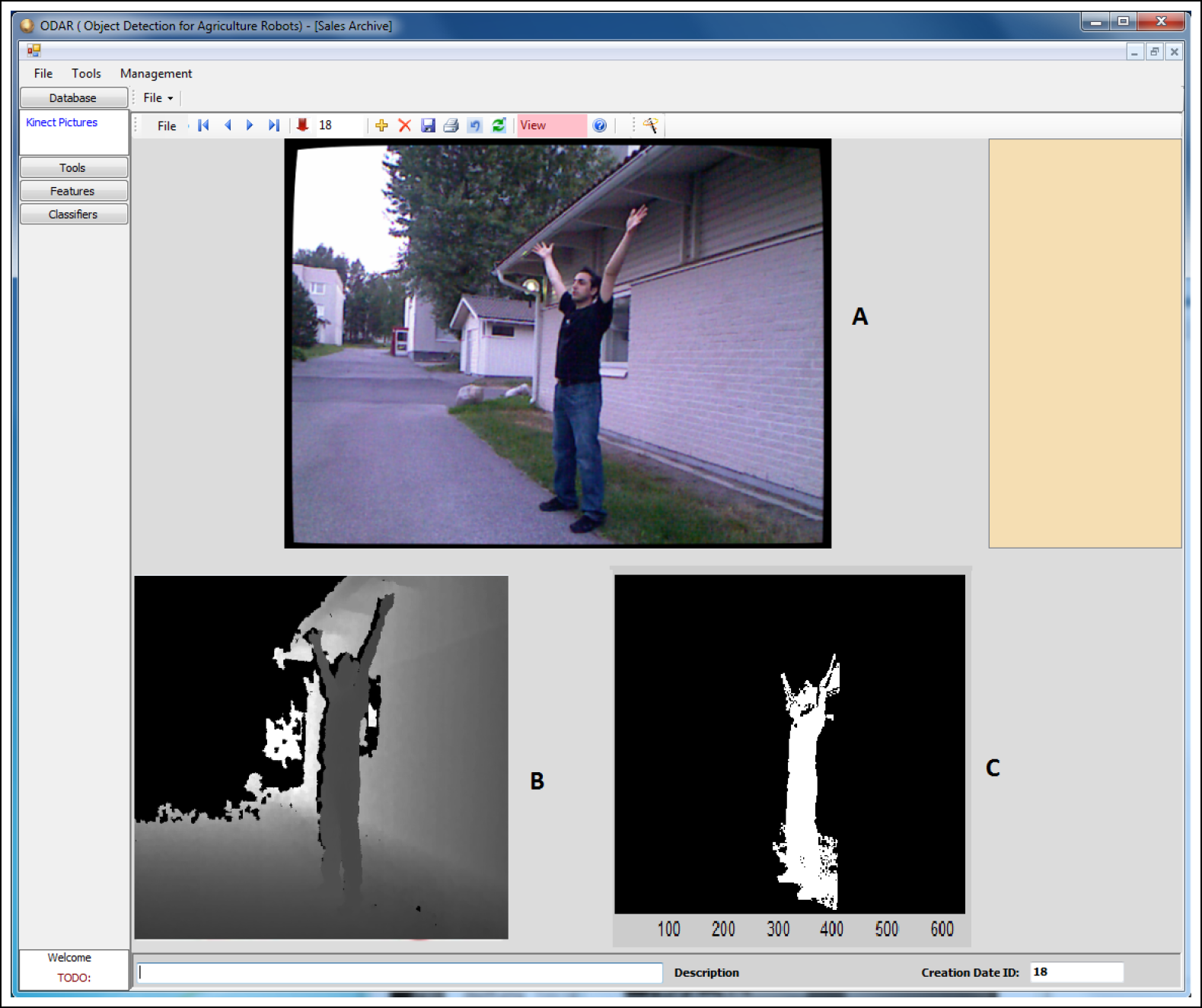
  17. Pordel, M.; Hellstrom, T.; Ostovar, A. Integrating Kinect Depth Data with a Stochastic Object Classification Framework for Forestry Robots, Proceedings of the 9th International Conference on Informatics in Control, Automation and Robotics, Rome, Italy, 28–31 July 2012.
  18. Zhang, K.; Zhang, L.; Song, H.; Zhou, W. Active contours with selective local or global segmentation: A new formulation and level set method. Image Vis. Comput. 2010, 28, 668–676. [Google Scholar]
  19. Dillencourt, M.; Samet, H.; Tamminen, M. General approach to connected-component labelling for arbitrary image representations. J. ACM 1992, 39, 253–280. [Google Scholar]
  20. Bezdek, J.C.; Ehrlich, R.; Full, W. FCM: The fuzzy c-means clustering algorithm. Comput. Geosci. 1984, 10, 191–203. [Google Scholar]
  21. Lim, Y.W.; Lee, S.U. On the color image segmentation algorithm based on the thresholding and the fuzzy c-means techniques. Pattern Recogn. 1990, 23, 935–952. [Google Scholar]
  22. Chuang, K.S.; Tzeng, H.L.; Chen, S.; Wu, J.; Chen, T.J. Fuzzy c-means clustering with spatial information for image segmentation. Comput. Med. Imaging Graph. 2006, 30, 9–15. [Google Scholar]
  23. Pham, D.L.; Prince, J.L. An adaptive fuzzy C-means algorithm for image segmentation in the presence of intensity inhomogeneities. Pattern Recogn. Lett. 1999, 20, 57–68. [Google Scholar]
  24. Zhang, D.Q.; Chen, S.C. A novel kernelized fuzzy C-means algorithm with application in medical image segmentation. Artif. Intell. Med. 2004, 32, 37–50. [Google Scholar]
  25. Veksler, O.; Boykov, Y.; Mehrani, P. Superpixels and supervoxels in an energy optimization framework, Proceedings of the 11th European Conference on Computer Vision, Part V, Heraklion, Greece, 5–11 September 2010; pp. 211–224.
Figure 1. Examples of extracted trees (A), stone (B), human (C), and bush (D). These object types are important for forestry robots and are the main focus of the work in this paper.
Computers 04 00142f1
Figure 2. Curve evolution algorithm for RGB image segmentation. Segmentation after 1 (A), 50 (B) and 150 (C) iterations.
Computers 04 00142f2
Figure 3. Curve evolution algorithm for depth image segmentation. Segmentation after 1 (A), 50 (B) and 150 (C) iterations.
Computers 04 00142f3
Figure 4. Image segmentation using an algorithm based on graph cuts for the RGB image in Figure 6A.
Computers 04 00142f4
Figure 5. Stone in Figure 6 is extracted using ECCL in interaction with user. A: 3 clicks with high similarity threshold. B: 10 clicks with low threshold.
Computers 04 00142f5
Figure 6. RGB (A) and depth (B) image of stone using Microsoft Kinect.
Computers 04 00142f6
Figure 7. RGB Image (A), depth image (B) and the object labeling result using thresholding on depth image (C). The extracted object includes noise from background.
Computers 04 00142f7
Figure 8. Superpixels for Figure 6. (A):Applied on an RGB image. (B):Superpixels presented with coloring.
Computers 04 00142f8
Figure 9. Fuzzy C-mean clustering for Figure 1 using four clusters and RGBDepth features that are: (A) grey and depth images; (B) R, G, B channels of an RGB image and depth image.
Computers 04 00142f9
Figure 10. Example of extraction of a human object, with user corrections. Several superpixels have been removed from the initial extracted area in the last row.
Computers 04 00142f10
Figure 11. Stone extraction using the image in Figure 6. See text for more details.
Computers 04 00142f11

