SeismicNoiseAnalyzer: A Deep-Learning Tool for Automatic Quality Control of Seismic Stations

Abstract

SeismicNoiseAnalyzer 1.0 is a software tool designed to automatically assess the quality of seismic stations through the classification of spectral diagrams. By leveraging convolutional neural networks trained on expert-labeled data, the software emulates human visual inspection of probability density function (PDF) plots. It supports both individual image analysis and batch processing from compressed archives, providing detailed reports that summarize station health. Two classification networks are available: a binary model that distinguishes between working and malfunctioning stations and a ternary model that introduces an intermediate “doubtful” category to capture ambiguous cases. The system demonstrates high agreement with expert evaluations and enables efficient instrumentation control across large seismic networks. Its intuitive graphical interface and automated workflow make it a valuable tool for routine monitoring and data validation.

1. Introduction

Seismic networks generate continuous data streams from hundreds of stations, which must be regularly evaluated to ensure the quality and the reliability of seismic observations. Among the adopted tools for this purpose are spectral diagnostics, such as Power Spectral Density (PSD) [1,2] and Probability Density Function (PDF) [3] plots, generally calculated for ground acceleration over a certain period of time (a day, a month, etc.). These plots provide insights into the short-term and long-term noise behavior of a station and are commonly used to identify issues such as instrumental degradation, incorrect metadata, and environmental disturbances [3].

Traditionally, the interpretation of these diagrams relies on expert visual inspection, which is time-consuming and subject to human variability. With the growing scale of national and regional seismic networks [4], manual evaluation of spectra becomes increasingly impractical.

In recent years, machine learning (particularly convolutional neural networks (CNNs)) has emerged as a powerful approach for image classification tasks [5,6,7]. By training CNNs on representative examples, it is possible to transfer expert knowledge into automated systems capable of interpreting complex patterns. Previous studies have demonstrated the potential of CNNs in seismological applications, including event detection [8], signal denoising [9], and noise classification in seismic survey [10].

In this context, we present SeismicNoiseAnalyzer 1.0, a software tool that automates the classification of seismic station spectra using pre-trained deep learning models [8,11,12,13]. The software supports both individual and batch classification of PDF diagrams, providing diagnostics and comprehensive reporting. Its goal is to streamline station quality control workflows and support network operators in identifying malfunctioning stations or suspect metadata. The present work follows [14], which introduced the neural network-based approach to the problem of seismic station quality. In contrast, the focus of this paper is on releasing the software, together with two already trained neural networks that were extensively discussed in the previous study. Hence, we refer to [14] with regard to the criteria used to classify a functioning or malfunctioning station (reliable data or not), as well as all the details about the neural network architecture used and the results in terms of accuracy.

2. Materials and Methods

The SeismicNoiseAnalyzer 1.0 software, designed for the automatic classification of seismic noise spectral diagrams, particularly probability density function (PDF) plots, builds upon deep learning methodologies. These plots are typically generated by the SQLX software package [15,16], which derives spectral diagrams from recorded time series at seismic stations. Such representations, in which transients such as earthquakes, spikes, etc. have a low probability of occurrence [3], are often employed by experts to assess the quality and reliability of the data [15]. SeismicNoiseAnalyzer 1.0 specifically operates on acceleration power spectra, one of the standard outputs provided by the SQLX package. This choice is relevant because both the interpretation of the spectral diagrams and their subsequent classification are inherently linked to this type of representation. It is important to state that, in the spectra we have used, the acceleration is computed as the derivative of broadband velocimeters (with high sensitivity) and not from the direct measure of accelerometers (having a low sensitivity) because generally they do not resolve the seismic noise. The system has been developed through the implementation of two neural networks trained under a deliberately conservative policy, privileging the classification of good stations as anomalous (false positives) over the converse (false negatives). This conservative strategy was achieved through cautious data labeling and classification procedures, ensuring more stringent reliability criteria [14]. Methodologically, the approach operates in two main stages. In the first, an expert provides a manual classification of a representative subset of spectra (e.g., labeled as OK or BROKEN). These labeled diagrams constitute the training dataset for the neural network, which thereby acquires the ability to discriminate between acceptable and anomalous spectra. Upon completion of the training phase, the network is capable of autonomously distinguishing valid spectral patterns from those indicative of malfunction or noise anomalies.

For SeismicNoiseAnalyzer 1.0, the following two convolutional neural networks were trained to perform the classification:

• A binary classifier (2-class), distinguishing between OK and BROKEN stations.
• A ternary classifier (3-class), distinguishing between OK, BAD, and an intermediate class DOBIOUSorTEMP to better account for ambiguous or borderline cases.

These networks correspond to the configurations that achieved the highest accuracies in the second and fourth experiments reported in [14]. For both classifiers, 20% of the data were reserved for testing and 10% for validation. The training dataset consists of images derived from data of real stations within the Italian Seismic Network (IV), the Mediterranean Network (MN), and more than 20 other collaborating regional and international networks (see https://terremoti.ingv.it/instruments), which data flows into the INGV seismic monitoring rooms. In this way, we use data from more than 600 European stations, and this covers most of the sismometers in use. Each PDF image summarizes the noise spectral behavior of one component of one seismic station over an extended period (for the training stage we choose one year): the image is generated by the SQLX package and derived from thousands of power spectral densities, computed on consecutive windows of 60 min. In this way, transient variations are integrated into a statistical representation of the station behavior. This procedure avoids assuming strict stationarity of the seismic noise, since the PDFs incorporate non-stationary dynamics by construction [3,15]. The images were selected by human experts using predefined criteria based on spectral trends [14], including comparisons against the Peterson Low Noise Model (LNM) and High Noise Model (HNM) [1], and patterns such as bimodal distributions, scattered spectra, not powered seismometer, etc. Images were not pre-processed or cropped; instead, they were used directly as input to the networks. This decision was made to maintain consistency with the visual cues that human experts use in manual inspection, such as overall spectral shape and distribution density.

The two neural networks released alongside the SeismicNoiseAnalyzer 1.0 software have been assessed according to the following metrics, which we briefly summarize here. The definitions provided refer to a binary classifier (with classes “positive” and “negative”) and should be analogously extended to multi-class classifiers. Let $TP$ (true positive) and $TN$ (true negative) denote the test samples correctly classified by the network as positive and negative, respectively, and let $FP$ (false positive) and $FN$ (false negative) denote the test samples misclassified by the network as positive and negative, respectively. The precision is defined as

$$\mathrm{Precision}={\displaystyle \frac{TP}{TP+FP}},$$

and it expresses the fraction of positive predictions that are correct. The recall measures the fraction of actual positives that are correctly detected and is calculated as

$$\mathrm{Recall}={\displaystyle \frac{TP}{TP+FN}}.$$

The F1-score is

$$F1=2·{\displaystyle \frac{\mathrm{Precision}·\mathrm{Recall}}{\mathrm{Precision}+\mathrm{Recall}}},$$

and it represents the harmonic mean of precision and recall, providing a balanced evaluation. Finally, the overall accuracy

$$\mathrm{Accuracy}={\displaystyle \frac{TP+TN}{TP+FP+FN+TN}}$$

determines how close a measured value is to the true or actual value. These metrics values regarding the two neural networks released are shown in

Table 1. Metric values for the two neural networks released alongside SeismicNoiseAnalyzer 1.0 software.

	Accuracy	Precision	Recall	F1-Score
Binary classifier	0.937	0.926	0.969	0.946
Three-class classifier	0.874	0.910	0.967	0.938

.

The classification models were implemented and executed within MATLAB^® (version 2024a), and this is now released in a stand-alone application.

Further details on the experimental design and hyperparameter tuning are beyond the scope of this work and can be found in [14].

3. Software Use

SeismicNoiseAnalyzer 1.0 offers a graphical user interface (GUI) designed for ease of use, targeting both technical personnel and researchers who require a rapid assessment of stations’ health. The software supports the classification of both individual PDF images and entire ZIP archives containing multiple PDF spectra. The result of a classification session is a detailed report that includes summaries and visual feedback.

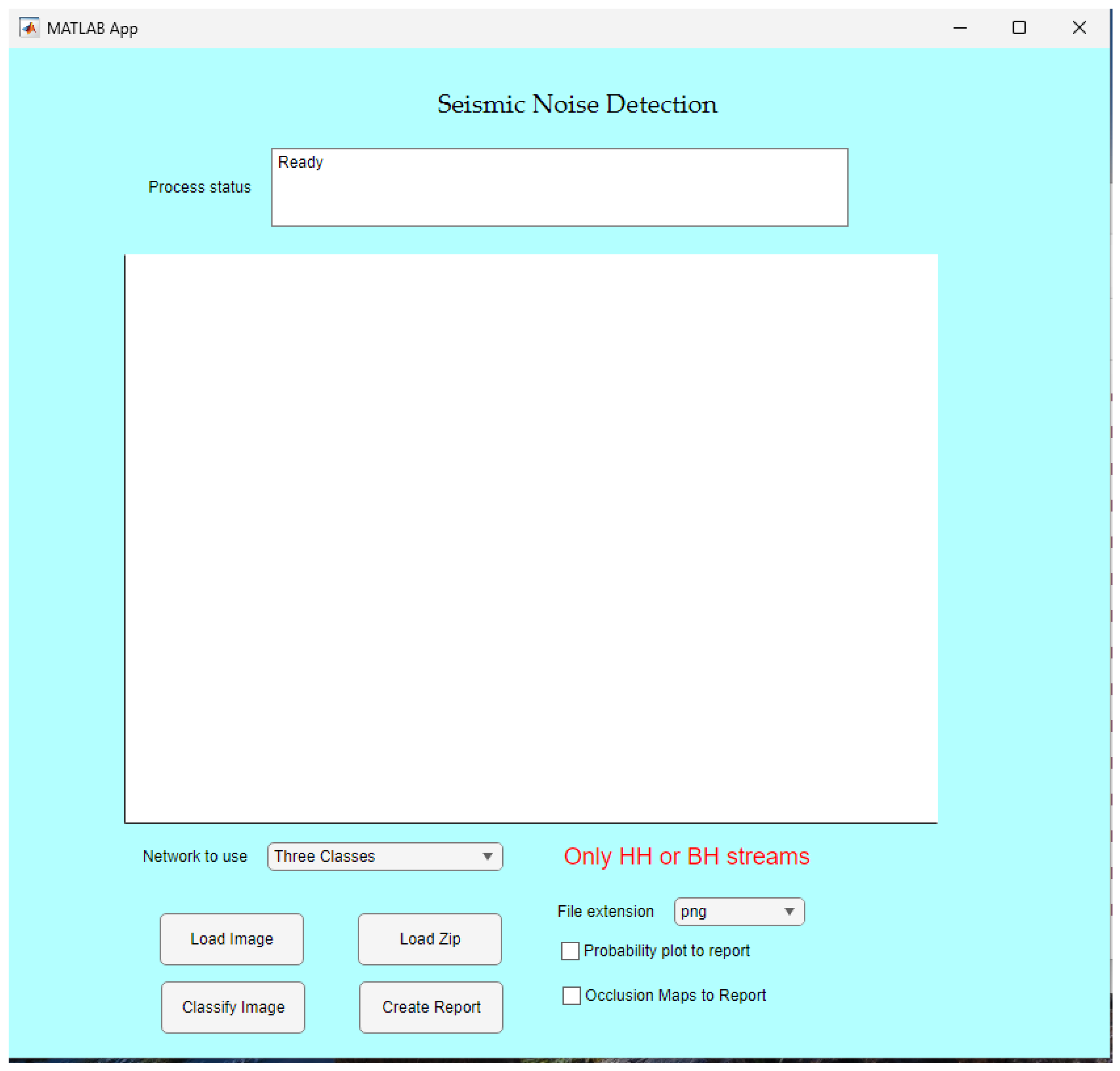
The GUI is structured into functional sections that guide the user through data selection, network choice (two or three classes), image classification, and report generation. Figure 1 shows the main interface layout.

3.1. Installation

SeismicNoiseAnalyzer 1.0 runs only on Microsoft^® Windows platform. The installation procedures require the user to register at geosoftware.sci.ingv.it, download the setup file, and follow the standard Windows installation steps. The program can then be executed either through the generated .exe file or by accessing it via the Windows Start menu. The administrator privileges are required; therefore, the application must be launched using the ‘Run as administrator’ option. When SeismicNoiseAnalyzer 1.0 starts, the GUI shown in Figure 1 will appear.

3.2. Input Data and File Format

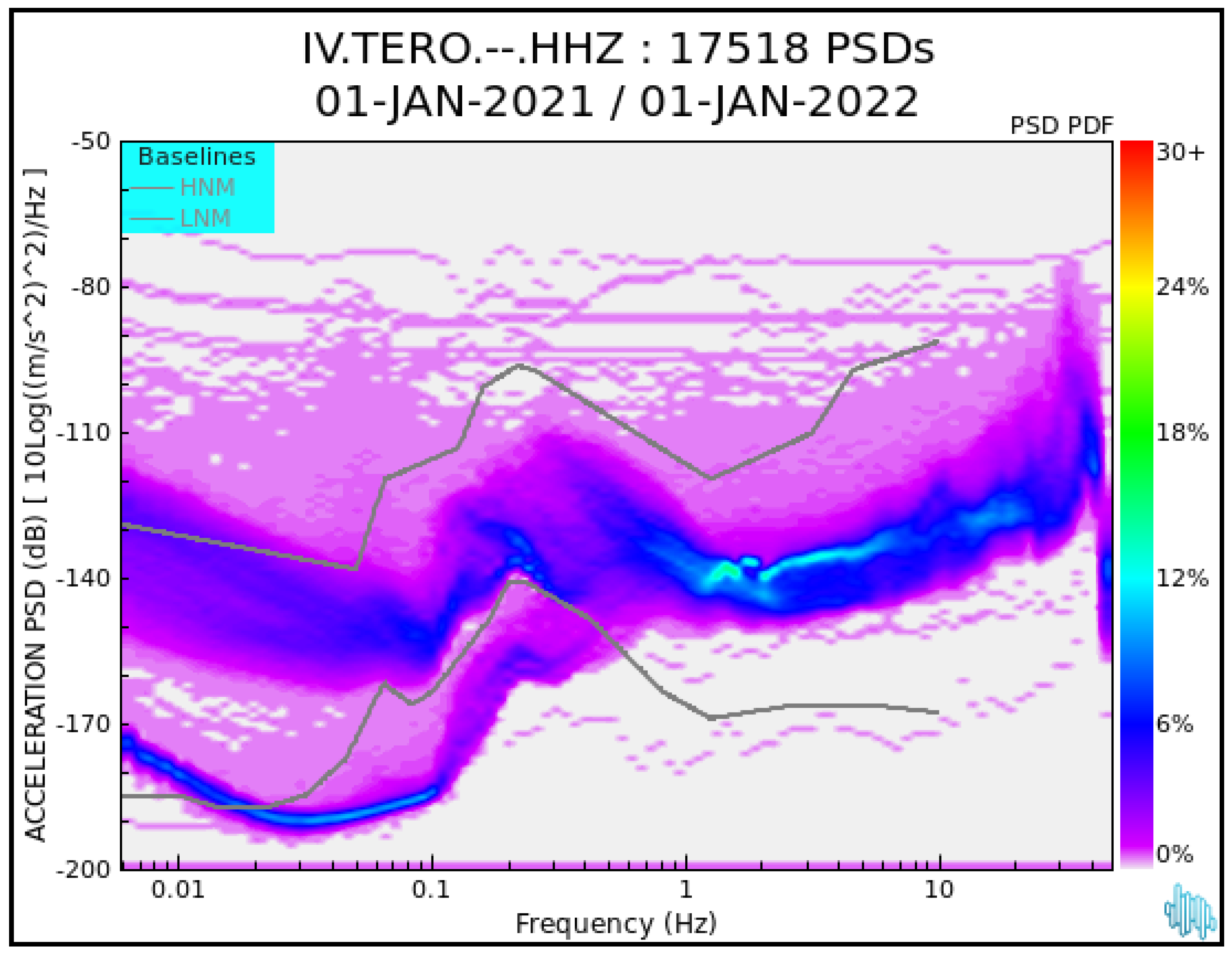
The input data for the classification are images in PNG or JPG format representing the annual or seasonal PDF distribution of the power spectral density for a specific seismic station and component. For broadband stations, normally the HH* channels are used [17], where HHZ is the vertical component, HHN is the North component, and HHE is the East component. Images regarding also channel BH* can be loaded. The plots contain frequency (Hz) on the x-axis and PSD values (dB) on the y-axis, with a color scale indicating statistical probability [15], as shown in Figure 2. Naturally, the input images can correspond to any broadband station belonging to any seismic network, as long as they exhibit the image features described above.

Users can select either a single image or a compressed ZIP archive containing multiple images, uploading them via buttons Load Image or Load Zip, respectively. The software automatically filters valid image files with .png or .jpg extensions according to the choice of the drop down menu File Extension.

3.3. Single-Image Classification

For a single-image classification, the spectrum has to be loaded using the Load Image button and manually selecting it from a file browser. The chosen image will appear in the GUI as in Figure 3. The choice of the classification to be performed, between the two-class or three-class neural networks as described in Section 2, can be made through the drop-down menu Network to use (see Figure 3). 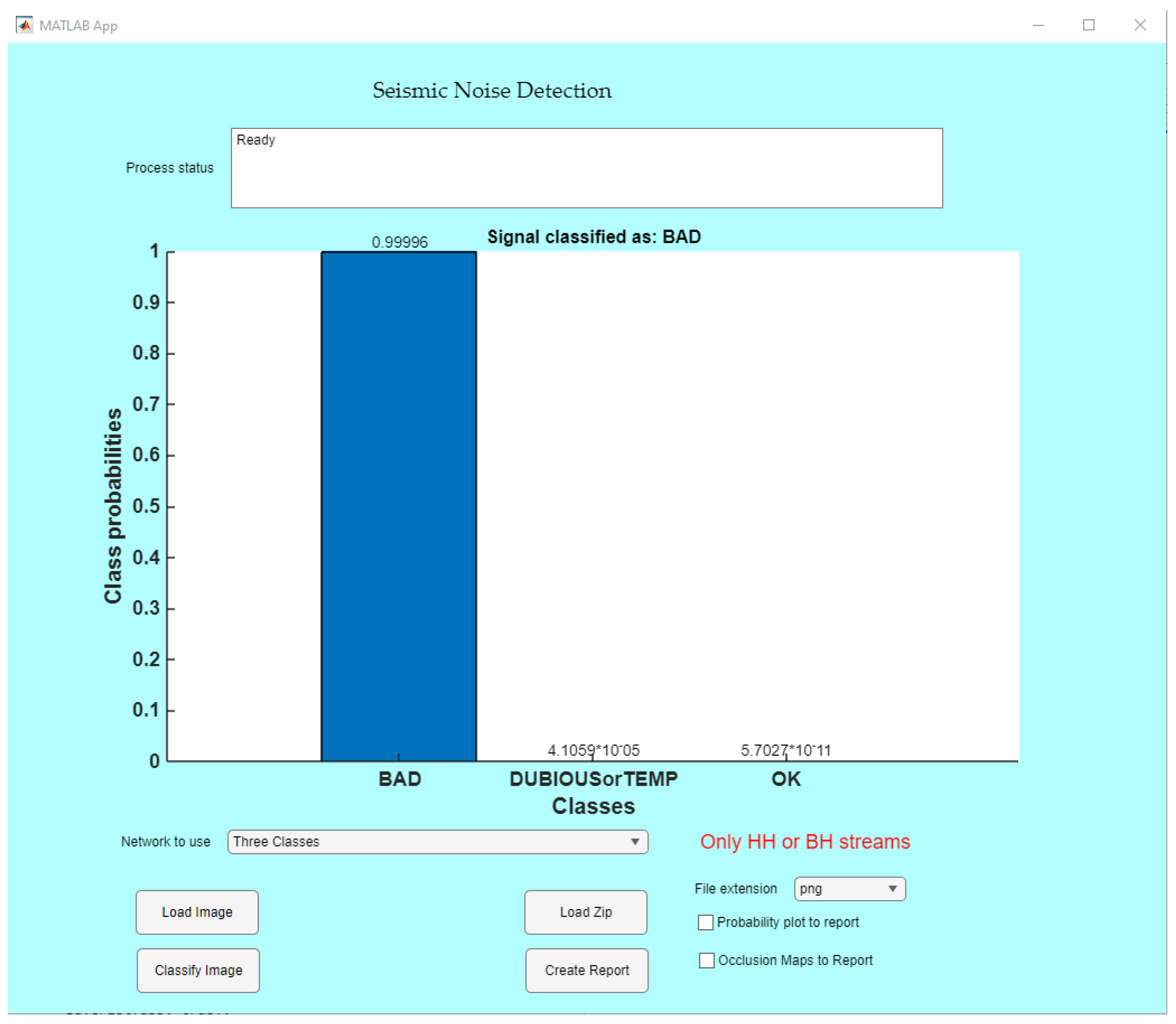Upon clicking on Classify Image, the output of the network is displayed in the GUI (Figure 4 and Figure 5). Specifically, a bar plot representing each class probability is shown so that the predicted label and the confidence score information can be retrieved.

Classifying a single image is ideal for inspecting problematic stations or validating specific edge cases by comparing classification outcomes with expert interpretation.

3.4. Batch Classification from Archive

For a batch classification, multiple images contained in a compressed ZIP archive can be loaded via Load Zip button. The software filters only the files with the extension selected by the drop-down menu File Extension. By the Create Report button, each filtered image is classified independently, again with respect to the chosen network in the drop-down menu Network to use. On the GUI, the image being processed by the network at a given time, together with the corresponding results, is displayed. Once all images have been processed, a ZIP archive containing the classification results, as described in Section 3.5, is automatically generated by the software, and the user is informed of the end of the operation by a message in the Process Status box.

A batch classification enables rapid screening of hundreds of station spectra, making it suitable for routine monitoring tasks and network-wide diagnostics.

3.5. Output Report and Export Options

When multiple images are classified simultaneously by uploading a ZIP file, the software returns another compressed archive containing four or five files (depending on the selected network), which list and summarize the classification results. The following files are included:

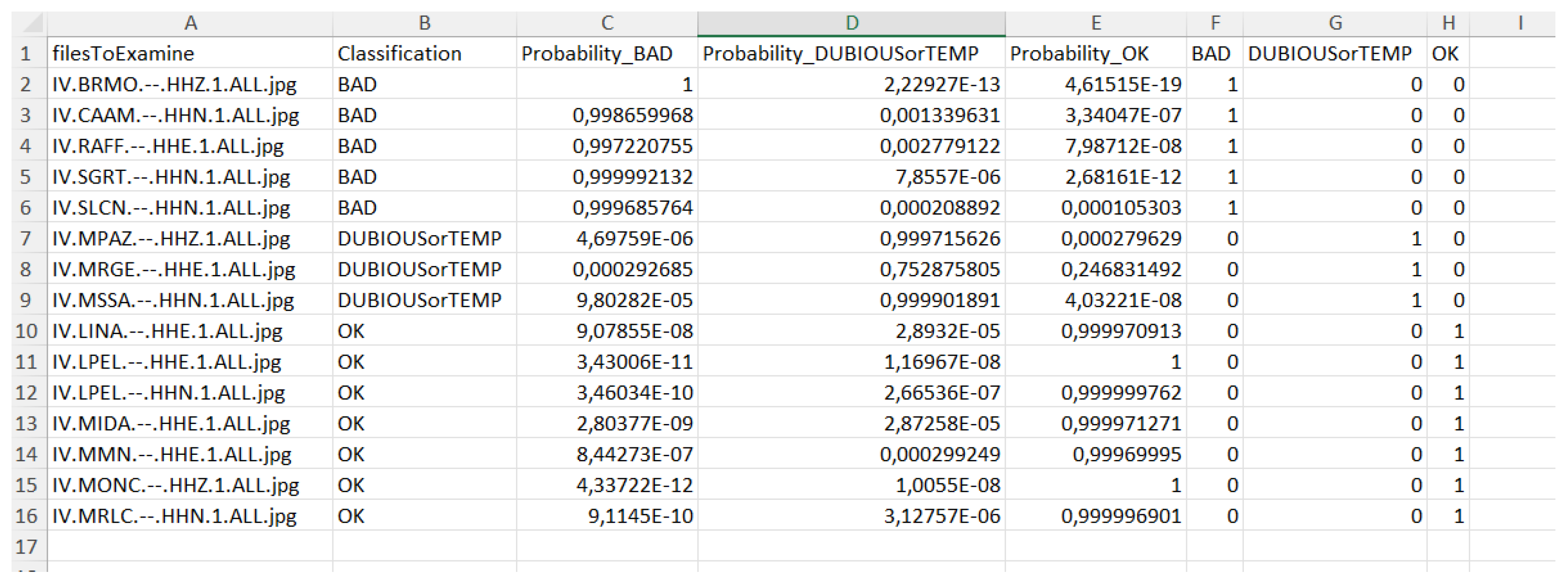
• “Reporttable.xlsx”: an Excel spreadsheet listing each input image along with its assigned classification and the associated probabilities for each class, as computed by the neural network (see Figure 6). This table enables users to inspect borderline cases and perform further filtering or sorting of results.
• “TheReport OK.pdf”: a .pdf file that lists all images classified as OK.
• “TheReport BAD.pdf” (or “TheReport BROKEN.pdf”): a .pdf file that lists all images classified as BAD (or BROKEN), generally indicating malfunctioning seismic stations or incorrect metadata.
• “TheReport DUBIOUSorTEMP.pdf”: a .pdf file containing all images classified as DUBIOUS or TEMPORARILY UNCLASSIFIABLE/TEMPORARILY BROKEN, typically due to many gaps, missing data (long latency), or insufficient duration. This file is produced only if the three-class network has been selected.
• “GeneralReport.pdf”: a .pdf file that provides an overall summary with the total number of processed images and the distribution across the classes (OK, BAD, BROKEN, and DUBIOUSorTEMP if applicable).

When either or both of the check boxes Probability plot to report and Occlusion Maps to Report are selected, the PDF reports described above will, for each image, additionally include the corresponding class probability bar plot and/or the occlusion sensitivity map. An occlusion sensitivity map (see Figure 7) is a diagnostic visualization technique employed to interpret the behavior of trained models, particularly in image classification tasks. It is generated by systematically masking small regions of the input and monitoring the corresponding variations in the model’s output. Input areas whose occlusion leads to substantial changes in the prediction are regarded as more influential, thereby enabling the identification of the regions most relevant to the model’s decision-making process [18].

4. Results

Extensive testing has demonstrated that the software is both efficient and robust, capable of handling large datasets without notable performance degradation and consistently delivering reliable results across diverse test scenarios. These characteristics render it well suited for integration into operational monitoring pipelines, where stability and resilience to imperfect data are essential.

As discussed in Section 2, the networks released with this software were trained following a precautionary strategy [14]. This means that, when misclassifications occur, they predominantly result in false positives (i.e., stations operating correctly but flagged as anomalous) rather than false negatives.

The performance of the proposed approach was one of the main focuses of [14], where four experiments were reported (see Table 2 in [14] for details). In one of these experiments, the network accuracy was evaluated on a set of 840 spectra using a model trained on data from different years in order to test its robustness under temporal variability.

Variations in noise levels or sensor characteristics are directly reflected in the spectral diagrams. For instance, at the TERO station, the seismometer was either unpowered or operated in short-period mode for a certain time interval, and the corresponding spectra clearly showed this behavior (see Figure 2). Consequently, its PDF image is classified as BROKEN/BAD.

These examples confirm that the tool not only maintains stable performance across large and heterogeneous datasets, but also that changes in station conditions leave recognizable patterns in the spectra, which can be reliably captured by the trained networks.

5. Discussion

The integration of deep learning into seismic data quality control marks a substantial step forward compared with traditional approaches. By leveraging pre-trained convolutional neural networks to emulate expert judgment, SeismicNoiseAnalyzer 1.0 overcomes one of the main constraints of manual inspection: scalability. As seismic networks expand in size and complexity, purely human-based monitoring becomes increasingly unsustainable.

In contrast to deterministic techniques that rely on RMS values, transmission gaps, or threshold-based filters, the classification of spectra (and, in the future, spectrograms) offers several advantages. It captures the complete spectral behavior over time, including frequency-dependent anomalies; it remains unaffected by raw count units or variability in station sensitivity, owing to the use of normalized (“deconvolved”) PSD values; and it reduces false alarms from transient disturbances or short gaps, since PDFs incorporate long-term trends.

The tool has proven particularly effective in detecting subtle forms of degradation, such as incorrect metadata (e.g., transfer function or sensitivity errors), out-of-level seismometers, and persistent shifts in environmental noise. In such situations, expert visual inspection of PDFs is often the only reliable diagnostic method, and the software reproduces this capability automatically.

Another important feature is the optional three-class classification scheme, which introduces an intermediate “doubtful” category. This functionality enables users to optimize resource allocation, prioritizing stations flagged as BAD while reserving ambiguous cases for expert review.

A recognized limitation of the approach lies in its dependence on the training dataset. Although the current models demonstrate robust generalization across years and networks, sustaining high performance in the long term will require periodic retraining, particularly as new instrumentation or changing site conditions emerge.

SeismicNoiseAnalyzer 1.0 is not intended to replace but rather to complement existing diagnostic tools. Issues such as time drift, polarity inversion, Azimuth error, or horizontal component mislabeling still require dedicated checks. Nevertheless, incorporating spectral inspection into a broader quality control framework can substantially reduce operational workload and enhance data integrity for downstream analyses.

Only a limited number of studies have so far explored the application of deep learning to seismic data quality control. For instance, ref. [10] employed supervised deep learning for general data quality characterization in seismic surveys (a collateral topic to this work), while [19] proposed a CNN-based image recognition approach to verify station efficiency. A very detailed comparison with [19] is present in [14]. Here, we briefly state that our methodology differs by using not preprocessed PDF diagrams as input, without the unstable mode curve, and coming from more than 20 seismic stations. Moreover, we adopt a conservative labeling strategy and perform extensive validation across multiple experiments. Finally, we release the software. To the best of our knowledge, SeismicNoiseAnalyzer 1.0 represents the first ready-to-use tool embedding a trained convolutional neural network specifically designed for the classification of seismic station noise diagrams and made directly available to the scientific community.

A related system was presented by [20], which focuses on the real-time quality control of Italian strong-motion data, generated by accelerometers. As a byproduct, it also analyzes many velocimetric stations, specifically those equipped with an accelerometer. Regarding data from velocimeters, the analysis, rather than on neural networks, relies on statistical thresholds defined over the entire network. The use of such thresholds, however, entails the risk of being either too strict or too permissive, whereas a neural network trained on individually classified images reduces this risk by learning from expert-labeled examples classified by spectrum shape.

Additional services exist, such as the EIDA portal described in [21], which provides rms values or other metrics for user-selected time periods. However, these metrics are not accompanied by an interpretative layer and do not directly indicate whether a station is functioning properly. In contrast, SeismicNoiseAnalyzer 1.0 delivers classification outcomes that explicitly inform on the operational status of seismic stations.

6. Conclusions

SeismicNoiseAnalyzer 1.0 provides an effective and efficient solution for automating the classification of seismic station spectra. Beyond this primary functionality, the tool has proven particularly valuable for detecting long-standing, previously unnoticed issues, such as metadata inconsistencies. Such overlooked problems are, in fact, more frequent than generally assumed. By leveraging convolutional neural networks trained on real examples curated by human experts, the software achieves classification accuracy that closely matches manual assessments, significantly reducing the time and effort required for routine station quality monitoring.

The ability to handle individual spectra as well as batch ZIP archives makes the tool flexible and suitable for both targeted investigations and large-scale analyses.

Although several open-source frameworks exist for implementing convolutional neural networks, they are not directly suited to the problem addressed here. Their use would require careful data selection, conservative labeling strategies, and dedicated training and evaluation procedures, all of which demand specific expertise. In contrast, SeismicNoiseAnalyzer 1.0 integrates already trained neural networks built on a curated dataset informed by expert knowledge. To the best of our knowledge, no other available neural network-based software provides a ready-to-use solution for assessing seismic station quality through PDF diagrams of recorded noise.

Further validation on broader datasets and the identification of potential edge cases remain objectives for future development. Nevertheless, the release of SeismicNoiseAnalyzer 1.0 already represents a significant advance in enhancing the efficiency of seismic noise analysis and in strengthening the operational monitoring of seismic networks. Moreover, its intuitive graphical interface and automated reporting system facilitate faster and more informed decision-making. In particular, while SeismicNoiseAnalyzer 1.0 does not substitute the role of network operators in deciding whether and when to intervene on malfunctioning stations, it already offers a clearer and more systematic overview of station performance, thereby supporting more informed and timely decision-making. At the same time, this advancement can be regarded as a first step toward future implementations of semi-automatic or fully automatic decision strategies, once sufficient experience and validation have been achieved.