Article

Time–Frequency Feature Fusion Approach for Hemiplegic Gait Recognition

by
Linglong Mao
* and
Zhanyong Mei
*
College of Computer Science and Cybersecurity, Chengdu University of Technology, Chengdu 610059, China
*
Authors to whom correspondence should be addressed.
Computers 2025, 14(8), 334; https://doi.org/10.3390/computers14080334
Submission received: 8 July 2025 / Revised: 3 August 2025 / Accepted: 11 August 2025 / Published: 18 August 2025
(This article belongs to the Special Issue Multimodal Pattern Recognition of Social Signals in HCI (2nd Edition))

Abstract

Accurately distinguishing hemiplegic gait from healthy gait is significant for alleviating clinicians’ diagnostic workloads and enhancing rehabilitation efficiency. The center of pressure (CoP) trajectory extracted from pressure sensor arrays can be utilized for hemiplegic gait recognition. Existing research studies on hemiplegic gait recognition based on plantar pressure have paid limited attention to the differences in recognition performance offered by CoP trajectories along different directions. To address this, this paper proposes a neural network model based on time–frequency domain feature interaction—the temporal–frequency domain interaction network (TFDI-Net)—to achieve efficient hemiplegic gait recognition. The work encompasses: (1) collecting CoP trajectory data using a pressure sensor array from 19 hemiplegic patients and 29 healthy subjects; (2) designing and implementing the TFDI-Net architecture, which extracts frequency domain features of the CoP trajectory via fast Fourier transform (FFT) and interacts or fuses them with time domain features to construct a discriminative joint representation; (3) conducting five-fold cross-validation comparisons with traditional machine learning methods and deep learning methods. Intra-fold data augmentation was performed by adding Gaussian noise to each training fold during partitioning. Box plots were employed to visualize and analyze the performance metrics of different models across test folds, revealing their stability and advantages. The results demonstrate that the proposed TFDI-Net outperforms traditional machine learning models, achieving improvements of 2.89% in recognition rate, 4.6% in F1-score, and 8.25% in recall.

1. Introduction

Hemiplegia is one of the most common sequelae following a stroke, typically presenting as unilateral motor dysfunction that significantly impacts a patient’s daily quality of life [1]. As such, accurately identifying gait characteristics in hemiplegic patients is essential for assessing the severity of the condition, developing personalized rehabilitation plans, and tracking rehabilitation progress [2]. However, current clinical evaluations largely rely on subjective physician observations and scale-based assessments, which are inherently biased and lack objective, quantifiable metrics to support the evaluation [3].
Recent advancements in sensor technology and artificial intelligence have led to the rise of hemiplegic gait recognition methods based on various sensing technologies. Researchers have employed single-point pressure sensors [4,5,6] and pressure sensor arrays [7,8] to capture gait-related data, enabling the objective quantification of gait parameters in patients. By combining these gait data with traditional machine learning or deep learning approaches, efficient models for recognizing hemiplegic gait can be developed, allowing for the automatic differentiation between hemiplegic and healthy gaits. This method offers valuable technical support for objective evaluation and auxiliary diagnosis.
Studies have shown that compared to healthy individuals, hemiplegic patients exhibit significant differences in plantar pressure distribution between the affected and unaffected sides, and these differences can be utilized to distinguish hemiplegic gait from healthy gait [9,10]. Although research on the gait differences between the affected and unaffected sides in hemiplegic patients has made some progress, studies focusing on the use of plantar pressure features for effectively differentiating between hemiplegic patients and healthy individuals remain relatively limited [7]. Among various sensing technologies, pressure sensor arrays are considered the ideal choice for plantar pressure measurements, owing to their high spatial and temporal resolution, as well as their excellent data stability. The plantar pressure distribution data collected by these sensor arrays not only capture dynamic changes in plantar pressure throughout the walking cycle but also enable the extraction of key spatiotemporal features, such as the pressure center trajectory. This offers a solid foundation for high-precision hemiplegic gait recognition. However, systematic explorations of how to leverage the pressure center trajectory extracted from pressure sensor arrays for effective hemiplegic gait identification remain insufficient.
To analyze the differences in the performance of time–frequency features extracted from center-of-pressure (CoP) trajectories in different directions for hemiplegic gait recognition, this study aims to develop a gait recognition model that integrates both time domain and frequency domain features. In addition, it compares the classification performance and computational efficiency of several deep learning models and traditional machine learning algorithms commonly adopted in related research studies. The main contributions of this work are as follows:
(1)
CDUT Plantar Pressure Dataset—Middle-Aged and Elderly Group (CDUT-PP-MAE): A dataset of plantar pressure data was collected from 48 middle-aged and elderly individuals, including both hemiplegic and healthy participants. Based on these data, a center of pressure trajectory dataset was constructed to validate the effectiveness of the proposed hemiplegic gait recognition method.
(2)
The study compares the performance of hemiplegic gait recognition using plantar pressure center trajectories in different directional orientations.
(3)
A novel temporal–frequency domain interaction network (TFDI-Net) is introduced. Its superiority is demonstrated through comparisons with traditional machine learning methods, as well as state-of-the-art deep learning techniques.
The remainder of this paper is organized as follows. Section 2 reviews related work. Section 3 presents the methodology, including data collection, feature engineering, and data augmentation. Section 4 reports experimental results, comparing the model performance, conducting ablation studies for TFDI-Net, and evaluating computational metrics such as the parameter count and training time. Finally, Section 5 concludes the study.

2. Related Work

In recent years, significant progress has been made in the research of hemiplegic gait recognition and analysis using pressure sensor arrays and wearable plantar pressure sensor systems. However, studies focusing on the use of plantar pressure center trajectories in different directional orientations for hemiplegic gait recognition remain relatively limited. Most wearable-based studies place pressure sensors inside shoes to collect plantar pressure data, which are then directly used in machine learning and deep learning methods for accurate classification and anomaly detection of different gait types.
For instance, Xie et al. [4] designed a gait analysis system based on a self-developed pressure insole and recruited six hemiplegic patients (including both left and right side hemiplegia) and six healthy volunteers to collect plantar pressure data. By dividing the gait phases and extracting the plantar pressure distribution and CoP trajectory, they constructed a 54-dimensional gait feature set. Features were selected using a Spearman correlation analysis and the Random Forest (RF) algorithm, and the RF classifier was employed to identify different gait types. Experimental results showed that this method could distinguish normal, left hemiplegic, and right hemiplegic gaits with 99% accuracy, demonstrating its efficient recognition ability in small sample scenarios. Potluri et al. [5] introduced a deep learning approach by using a stacked long short-term memory (LSTM) network to build a temporal model for recognizing various abnormal gait types associated with neurological disorders. The study recruited ten healthy volunteers, who were instructed to simulate typical gait disorders, including hemiplegic, Parkinsonian, and sensory–ataxic gaits. The model’s training and validation results indicated high discriminative performance in abnormal gait recognition, with significant differences in the R2 regression metric between normal and abnormal gaits. Additionally, gait parameters such as the stance phase ratio, step frequency, and step time also exhibited consistent differences.
Cui et al. [8] combined the Bertec force platform, Qualisys motion capture system, and Biomonitor ME6000 system to collect tri-modal data from 21 stroke patients and 21 healthy individuals. Using random forest and support vector machine (SVM) algorithms, they achieved a high recognition rate of 98.21%, demonstrating the advantages of multimodal fusion. Lemoyne et al. [7] collected approximately 25 gait data samples from one hemiplegic patient using an AMTI pressure array. Despite the limited sample size, the study achieved 100% accuracy under leave-one-out cross-validation, highlighting the practical potential of logistic regression models in differentiating between the affected and unaffected sides. Rastegarpana et al. [11] further combined the VICON MX motion capture system with the Kistler 3D force platform to analyze the differences between “targeted steps” (goal-directed steps) and regular walking in stroke patients and healthy individuals. The results revealed that target steps were characterized by reduced step speed and shortened step length, suggesting that hemiplegic patients may adopt different motor control strategies in specific situations.
Kokolevich et al. [12] embedded plantar pressure sensors into the shoes of patients to collect ground reaction force (GRF) data during gait. The study involved two ischemic stroke patients (aged 59 and 73) who were both in the post-stroke recovery phase, six months after the stroke. The focus of the study was to compare the weight-bearing differences between the affected and unaffected sides in the forefoot and hindfoot regions. The analysis revealed that the ground reaction forces in the fore and hindfoot regions of the affected side were lower than those on the unaffected side, with a particularly noticeable asymmetry during the toe-off and heel-strike phases. Notably, some patients exhibited a degree of insufficient weight-bearing even on the unaffected side. This suggests that stroke-induced gait abnormalities not only affect the weight distribution on the affected side but may also impair the weight-bearing mechanism of the contralateral lower limb. Hayashi et al. [6] designed a wearable plantar pressure biofeedback system (PEBF) and recruited six hemiplegic patients (mean age 56.8 ± 11.4 years) at the Tokyo General Hospital for a 3 week walking intervention, consisting of three 20 min sessions per week. Post-intervention, the patients showed a significant increase in the step length of the affected side (p = 0.0277) and a marginal improvement in the plantar flexion angle of the affected side (p = 0.0747), indicating the potential of the PEBF system in improving the push-off function in gait.
In rehabilitation intervention studies for hemiplegic patients, Park et al. [13] used the GAITRite gait analysis system to collect plantar pressure data from hemiplegic patients while wearing shoes. Through an analysis of gait parameters and plantar pressure distribution, they suggested that changes in plantar pressure distribution induced by the intervention may play a positive role in improving gait symmetry and regulating postural balance. Kim et al. [14] conducted a comparative analysis of initial and follow-up gait data from two groups of patients to assess their gait recovery progress. The study found that left- and right-side hemiplegic patients exhibited differences in the rate of gait recovery, which might be related to the habitual use of body balance and compensatory mechanisms in right-handed patients. Therefore, rehabilitation training for hemiplegic patients should fully consider the differences between the affected sides and develop more individualized gait intervention strategies to further enhance recovery outcomes and improve the patients’ quality of life.

3. Materials and Methods

In this study, the Footscan pressure sensor array system was used to collect plantar pressure data from 48 middle-aged and elderly participants at the Second Affiliated Hospital of Chengdu Medical College. The plantar pressure center trajectories were then extracted from the data, and data augmentation techniques were applied to expand the training set samples. Additionally, the effectiveness of the proposed TFDI-Net was validated through comparisons with recent deep learning and machine learning methods. The overall workflow of the study is shown in Figure 1.

3.1. Data Acquisition from Student Participants

The data used in this experiment were collected using the Footscan plantar pressure measurement system (RSscan, Paal, Belgium), with a sampling rate of 253 Hz. The dataset, comprising both healthy and hemiplegic middle-aged and elderly individuals, was obtained from participants at the Second Affiliated Hospital of Chengdu Medical College under a 7 m straight-line walking protocol. The subjects included 19 hemiplegic patients and 29 healthy individuals, all of whom were able to walk independently without assistive devices or support. Detailed information about the dataset is provided in Table 1. The participants ranged in age from 50 to 77 years, with heights ranging between 1.5 and 1.78 m, weights ranging between 43 and 87 kg, and shoe sizes ranging from EU 36 to 42.
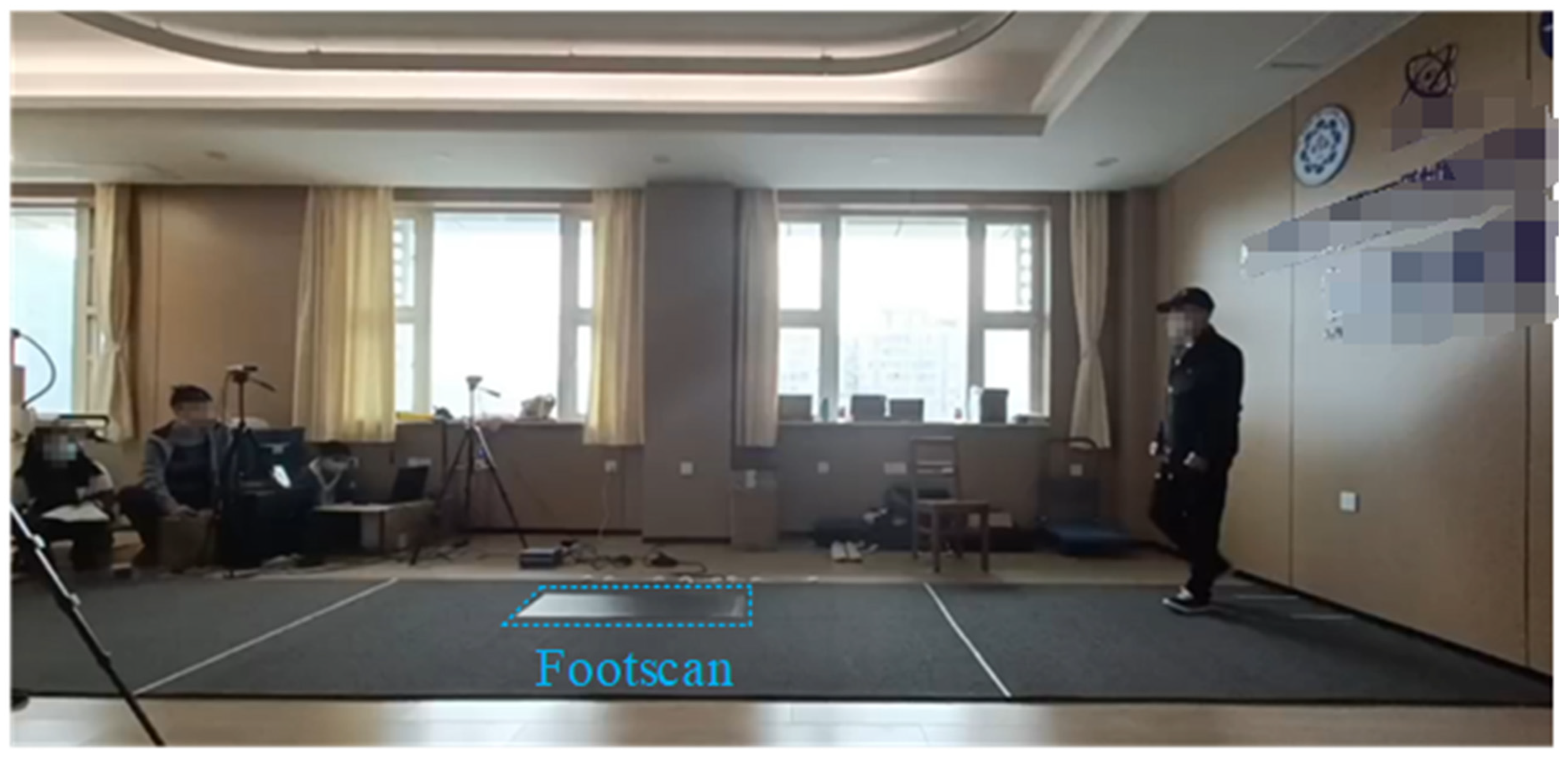
The experimental procedure adhered to the principles of the Declaration of Helsinki. Prior to participation, each subject was informed of the experimental protocol and provided written consent for data collection. Medical personnel were present throughout the entire procedure to ensure participant safety. Given the age-related decline in physical function, particularly among some hemiplegic patients who exhibited unstable gait, the data collection sessions for middle-aged and elderly participants were shorter in duration compared to those typically conducted with younger individuals. To minimize the influence of external factors on the experimental data, all participants walked on a standardized mat surface and were instructed to complete six straight-line walking trials at their natural, self-selected walking speed along a designated path. The data collection was conducted indoors, with the walking path set to a straight 7 m distance, following the 7 m walk test protocol. The experimental setup is illustrated in Figure 2.

3.2. Feature Engineering

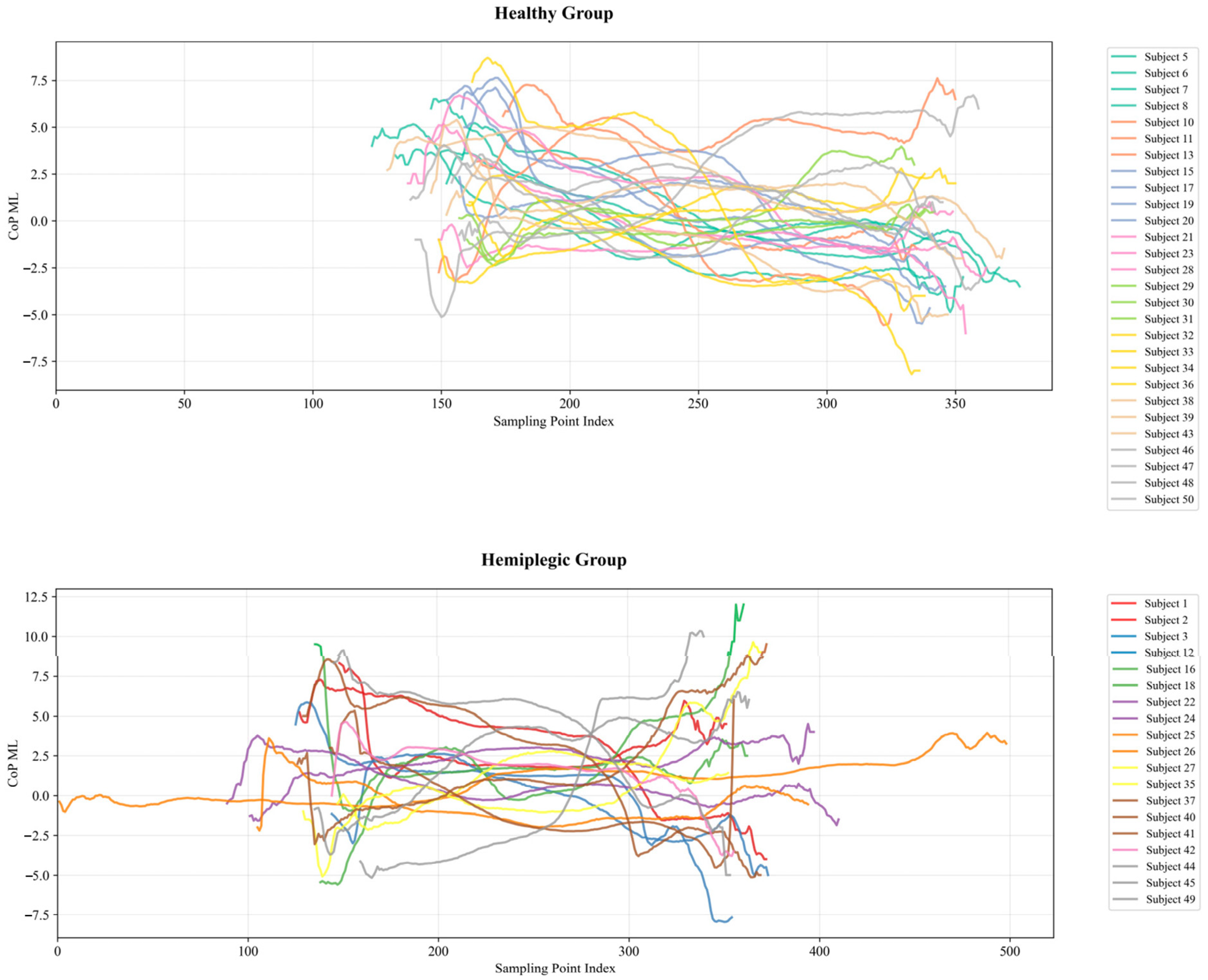
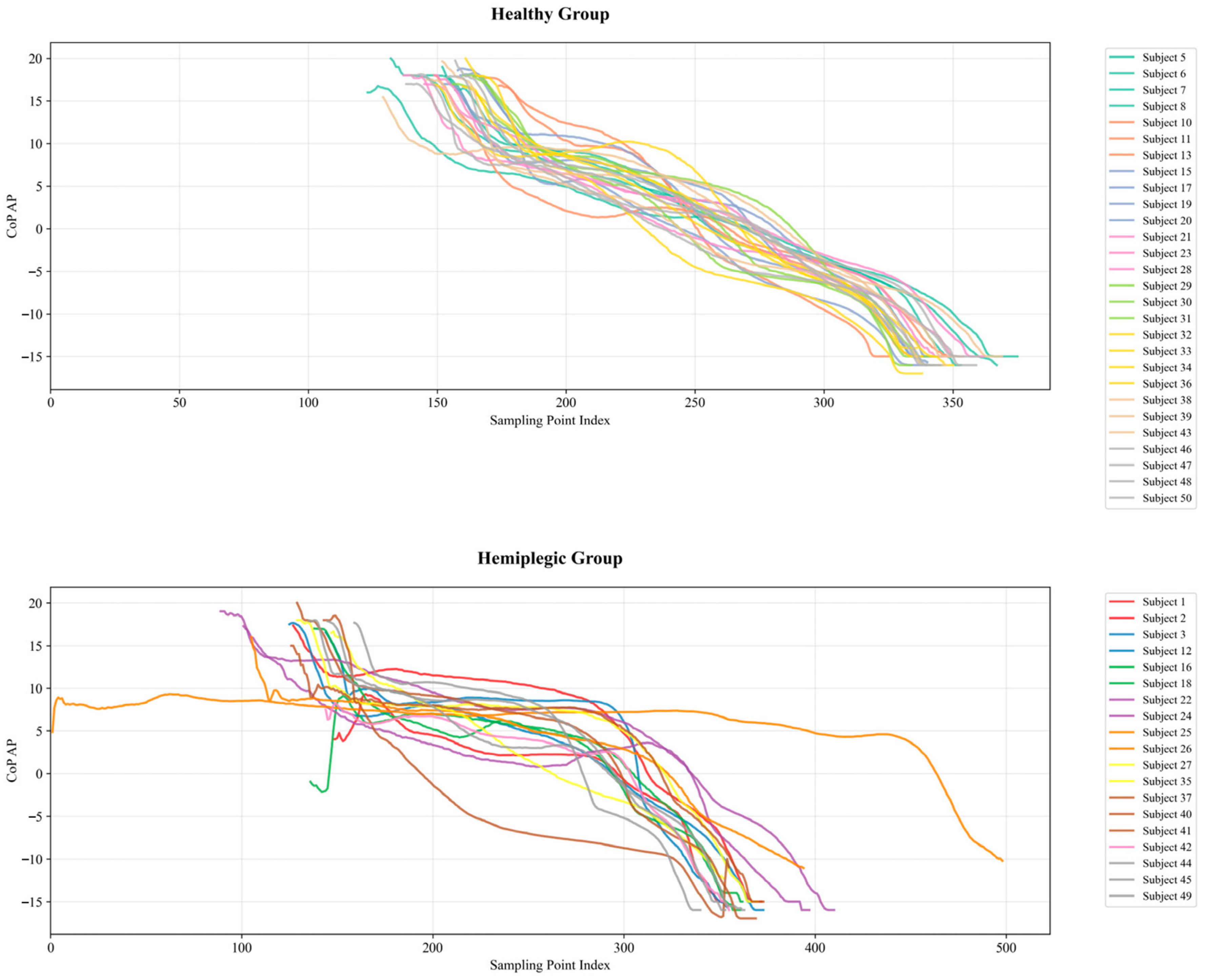
To compare the performance of machine learning and deep learning methods in hemiplegic gait recognition, statistical features were separately extracted from the anterior–posterior (AP) and medial–lateral (ML) CoP trajectories in both the time and frequency domains. Equations (1) and (2) present the calculation methods for the CoP trajectories in the ML and AP directions, respectively, while Figure 3 and Figure 4 illustrate the corresponding trajectories collected from the subjects. The time domain features included the mean, standard deviation, maximum, and minimum values. The frequency domain features included the dominant frequency, low-frequency energy, mid-frequency energy, high-frequency energy, and spectral entropy. The detailed computation processes are presented in Equations (3)–(11).
C o P M L = P i , j X i P i , j
C o P A P = P i , j Y i P i , j
x ¯ = 1 N i = 1 N x i
s t d = 1 N i = 1 N ( x i x ¯ ) 2
A m p l i t u d e = a b s ( m a x ( C o P   T r a j c t o r y ) m i n ( C o P   T r a j c t o r y ) )
Z e r o   C r o s s i n g   R a t e = 1 2 N n = 1 N 1 | s g n ( x [ n ] ) s g n ( x [ n 1 ] ) |
S a m p l e   E n t r o p y ( m , r ) = l n A B
v ¯ = 1 ( N 1 ) Δ t i = 1 N 1 | x i + 1 x i |
R M S = 1 N i = 1 N x i 2
f d o m i n a n t = a r g m a x f P ( f )
E l o w = f i < 1 P ( f i ) i = 1 N P ( f i )
E m i d = 1 f i < 3 P ( f i ) i = 1 N P ( f i )
E h i g h = f i 3 P ( f i ) i = 1 N P ( f i )
H = i = 1 N P ^ ( f i ) log 2 ( P ( f i ) j = 1 N P ( f j ) )
In Equations (1) and (2), P i j represents the pressure value of the sensor unit located in the i-th row and j-th column on the FootScan pressure plate, while X i and Y i denote the row and column indices, respectively. In Equations (3) and (4), x i denotes the i-th point in the CoP trajectory, and N represents the total number of samples. In Equation (6), x[n] represents the signal value of the n-th sample point in the CoP trajectory, sgn(⋅) denotes the sign function, and N is the total length of the signal. In Equation (7), A represents the proportion of sample pairs with a similarity distance less than r when the template length is m + 1, and B represents the proportion when the template length is m. The tolerance threshold r is defined as r r a t i o σ , where σ is the standard deviation of the signal, and m is the embedding dimension. In Equation (8), N denotes the total number of sampling points in the time series, x i represents the value at the i-th sampling point, and Δ t is the time interval between two adjacent sampling points. In Equation (9), x i represents a time point in the CoP trajectory.
In Equations (10)–(14), P ( f i ) represents the power spectral density, f d o m i n a n t the dominant frequency, E l o w the low-frequency energy, E m i d the mid-frequency energy, E h i g h the high-frequency energy, and H the spectral entropy.

3.3. Experimental Setup

A total of 50 participants were initially recruited for the study. After excluding one patient with bilateral hemiplegia and another with an insufficient number of samples, the final dataset included 29 healthy individuals and 19 hemiplegic patients. A subject-wise strategy was employed to partition the dataset into training and testing sets. To ensure an objective evaluation of the model’s ability to distinguish between hemiplegic and healthy gait patterns, five-fold cross-validation was performed, and the average values of all performance metrics across the folds were reported as the final results. During model training, the number of epochs was set to 100, and an early stopping strategy was implemented to prevent overfitting. For deep learning models, the initial learning rate was set to 1 × 10⁻⁴, and the Adam optimizer was used. A ReduceLROnPlateau scheduler was applied with a learning rate decay factor of 0.1 and a weight decay of 1 × 10⁻³. For machine learning models, optimal hyperparameters were determined using a grid search. The model was trained using an NVIDIA 3070 Ti GPU, Intel Core i7 12th-generation CPU, with PyTorch version 2.1.0 and Python version 3.8.
Six evaluation metrics were used to assess the performance of the models, including the accuracy, precision, F1-score, area under the ROC curve (AUC-ROC), specificity, and recall. The formulas for each metric are provided in Equations (15)–(20). In addition, confusion matrices were used to provide a more intuitive visualization of the differences in hemiplegic gait recognition performance across different methods.
A c c u r a c y = T P + T N T P + T N + F P + F N
P r e c i s i o n = T P T P + F P
F 1   S c o r e = 2 × P r e c i s i o n × R e c a l l P r e c i s i o n + R e c a l l
S p e c i f i c i t y = T N T N + F P
A U C = 0 1 T P R ( F P R ) d ( F P R )
R e c a l l = T P T P + F N
To comprehensively validate the effectiveness of the proposed method, the following representative traditional machine learning and deep learning approaches were selected as baseline models for comparison: support vector machine (SVM) [15], random forest (RF) [16], XGBoost [17], EfficientNetV2 [18], transformer [19], ResMLP [20], and long short-term memory (LSTM) network [21].

3.4. Data Augmentation

To enhance the model’s robustness to outliers and perturbations, a Gaussian noise-based data augmentation strategy was incorporated during training set construction. Considering that each fold in the cross-validation process involves a different subset of participants, an in-fold augmentation strategy was adopted to prevent data leakage. Specifically, data augmentation was performed independently within each training fold, rather than applying augmentation to the entire dataset prior to cross-validation. This approach ensured complete separation between training and validation data, thereby improving the reliability during model evaluation. For each original training sample, N augmented replicas were generated by introducing small perturbations. Gaussian noise sampled from a normal distribution was added to the original sequences to simulate real-world variability in data acquisition and sensor errors. The detailed procedure is illustrated in Algorithm 1.
Algorithm 1: Gaussian Noise-Based Data Augmentation
Input:
          X: Original time series sample ∈ T × D
          N: 5//Number of augmented copies
           σ m i n , σ m a x : 0.01, 0.05//Minimum and maximum noise standard deviation
Output:
          Augmented dataset D a u g containing N noisy copies of X
1
Initialize D a u g ← ∅
2
for i = 1 to N do
3
    Sample σ ∼ Uniform( σ m i n , σ m a x )
4
    Generate Gaussian noise: ε𝒩 (0, σ2), shape = (T, D)
5
    Add noise: X ~ X + ε
6
    Compute A ← max(abs(X))
7
    Clip X ~ within [−1.5A, 1.5A]
8
    if ∃ x X ~ such that x then
9
        Replace X ~ X
10
    end if
11
    Append X ~ to D a u g
12
end for
13
return D a u g

3.5. TFDI-Net

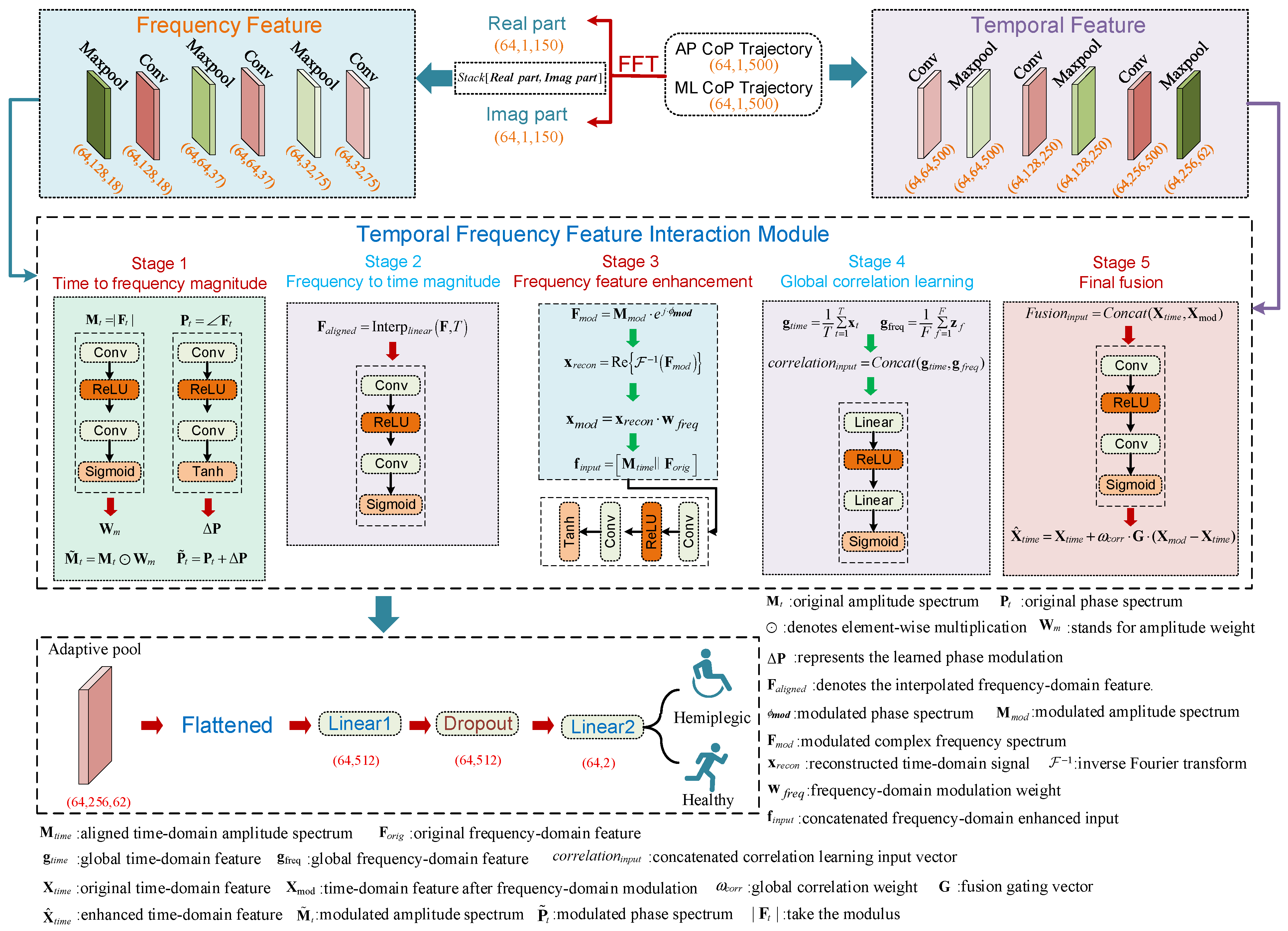
In this study, we propose a novel hemiplegic gait recognition network architecture that integrates temporal and frequency domain information, termed TFDI-Net (temporal–frequency domain interaction network). The network comprises three primary functional modules: a temporal domain convolution module, a frequency domain feature extraction module, and a temporal–frequency interaction module, which collaboratively enables multiscale feature fusion and complementary enhancement. The overall architecture of the TFDI-Net is illustrated in Figure 5 and its parameter settings are provided in Table 2.

3.5.1. Temporal Domain Convolution Module

To effectively capture the temporal structure of gait signals, TFDI-Net incorporates a temporal convolution module, as illustrated in the upper-right part of Figure 5, to model local dependencies and dynamic variation patterns within time series data. This module consists of a three-layer stacked one-dimensional convolutional architecture, where each convolutional layer is followed by a ReLU activation function and a max-pooling operation. This design enhances nonlinear feature extraction and facilitates efficient temporal downsampling.
Specifically, the input gait time series signal is first passed through a one-dimensional convolutional layer to extract low-level temporal features. These features are then further refined through a second and third convolutional layer, progressively deepening the temporal representation. Each convolutional layer uses a kernel size of 5, a stride of 1, and a padding of 2 to preserve the original sequence length. The max pooling operation following each convolution not only reduces the computational complexity but also enhances the robustness to temporal shifts. The computation process of this module can be formally expressed as follows:
H i + 1 = M a x p o o l ( R e L U ( C o n v i ( x ) ) )
Here, C o n v i denotes the i-th (i = 1, 2, 3) one-dimensional convolutional operation, with the numbers of output channels set to 64, 128, and 256, respectively. The final output of the temporal convolution module is fed into the subsequent attention module and the temporal–frequency interaction module for further feature fusion and modeling.
The parameter configuration of this module draws inspiration from the classical architectural design of the temporal convolutional network (TCN) [22], which has demonstrated stability and strong generalization performance across various biosignal processing and time-series classification tasks. Accordingly, this study adopts TCN’s convolutional kernel size and hierarchical channel configuration strategy. Preliminary experiments further confirmed the suitability of this structure for the gait recognition task.

3.5.2. Frequency Domain Feature Extraction Module

Temporal signals often contain rich frequency domain information that is not readily accessible in the time domain. To fully exploit the spectral characteristics of the gait signals, a frequency domain feature extraction module based on the fast Fourier transform (FFT) was designed in this study, as illustrated in the upper-left part of Figure 5. The core idea of this module is to transform the input from the time domain to the frequency domain using FFT, thereby extracting informative spectral features. Given an input time domain signal x ( t ) B × T , where B is the batch size and T is the sequence length, the module applies the discrete Fourier transform to each sample as follows:
X ( k ) = n = 0 T 1 x ( n ) e j 2 π k n / T ,         k = 0 , 1 , , T 1
To fully preserve the complex-valued information from the Fourier transform, the module decomposes the complex frequency domain coefficients into their real and imaginary parts:
F r e a l ( k ) = ( X ( k ) ) ,         F i m a g ( k ) = ( X ( k ) )
The final output of the frequency domain feature extraction module is denoted as F B × 2 × K , where the second dimension corresponds to the real and imaginary components of the frequency domain features, respectively. This design allows the module to effectively capture the spectral characteristics of the signal, providing valuable frequency domain information for subsequent feature fusion and classification tasks.

3.5.3. Temporal–Frequency Modal Interaction Module

To model the intrinsic correlation between time and frequency domain features of gait signals, we designed a cross-modal interaction module that enables bi-directional guidance and gated fusion between the two domains. The overall structure of the interaction module is illustrated on the middle of Figure 5, and the parameter settings of its submodules are provided in Table 2. The module consists of five key components:
(1)
Time-to-Frequency Guidance
The time domain features are first transformed using the fast Fourier transform (FFT) to obtain the magnitude and phase spectrum. Two modulation branches are then applied—one using a sigmoid function for magnitude and the other using a tanh function for phase—to generate adaptive modulation weights, enabling the dynamic refinement of frequency domain information.
(2)
Frequency-to-Time Guidance
The frequency domain features are interpolated to match the temporal resolution and passed through a learnable modulation branch to guide the reconstruction of time domain signals from the modulated spectral features.
(3)
Frequency Feature Enhancement
The magnitude spectrum derived from the time domain FFT is concatenated with original frequency features and passed through nonlinear transformations to produce enhanced frequency domain representations.
(4)
Global Time–Frequency Correlation Learning
Global average pooling is applied to both time and frequency features to obtain compact representations. These are fused via a lightweight MLP to compute a scalar correlation weight, representing the semantic alignment between the two modalities.
(5)
Gated Fusion
The original and modulated time domain features are concatenated and passed through a gating network. The final time domain representation is computed by weighting the fusion result using the learned correlation.
This module enables dynamic, bidirectional interactions between temporal and spectral cues, allowing the network to extract more discriminative and robust features for hemiplegic gait recognition.

4. Results

4.1. Hemiplegic Gait Recognition Results Based on CoP Trajectories

To investigate the differences in hemiplegic gait recognition performance between AP and ML CoP trajectories, experiments were conducted using both traditional machine learning methods and recent deep learning approaches. The results for accuracy, precision, and other metrics are presented in Table 3 and Table 4, respectively. The results demonstrate that TFDI-Net consistently achieved the best performance on both the AP and ML CoP trajectory datasets. Moreover, the experiments indicate that CoP trajectories in the AP direction are more informative and effective for recognizing hemiplegic gait.

4.1.1. Analysis of CoP Trajectory Recognition Results Using Machine Learning Methods

In this study, three machine learning algorithms—a support vector machine (SVM), random forest (RF), and XGBoost—were employed to classify hemiplegic gait based on time domain and frequency domain features extracted from AP and ML CoP trajectories. Through feature engineering, the raw trajectory data were transformed into 12-dimensional feature vectors, encompassing both statistical characteristics in the time domain and spectral features in the frequency domain. A five-fold cross-validation strategy was used to evaluate model performance.
The results revealed significant differences in recognition performance across the three algorithms when applied to AP and ML CoP trajectory data. Overall, for the AP direction, the SVM algorithm outperformed the others across all evaluation metrics, followed by RF, with XGBoost performing the worst. In contrast, for the ML direction, the SVM algorithm achieved the best performance on all metrics, followed by XGBoost, while RF yielded the poorest results.
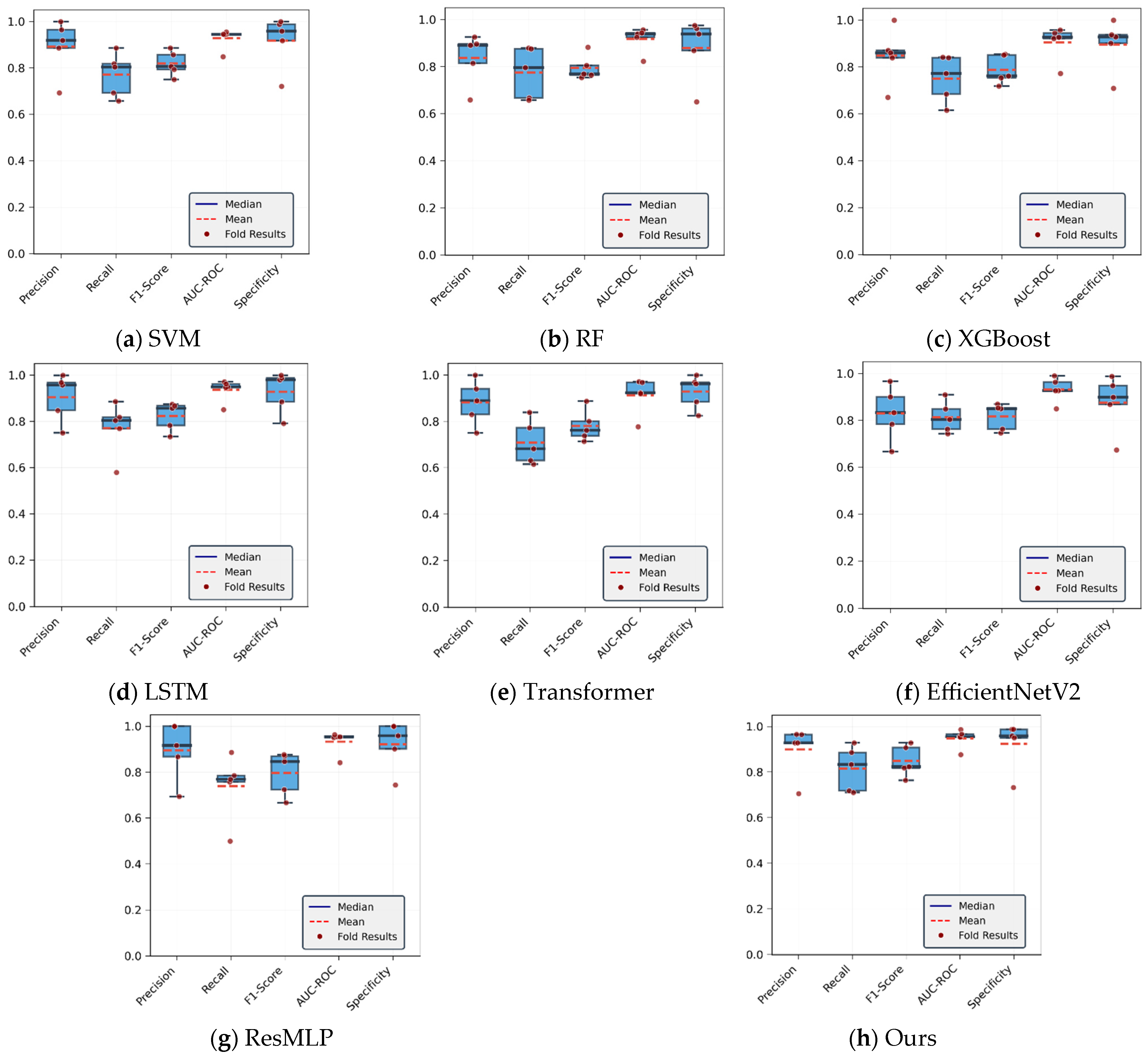
SVM demonstrated the best performance on the AP CoP trajectory, which can be primarily attributed to the algorithm’s strong compatibility with the 12-dimensional feature space. First, SVM is known for its excellent classification capability in low- to medium-dimensional feature spaces, where it can identify the optimal separating hyperplane. Second, given the relatively limited sample size in this study (29 healthy subjects and 19 hemiplegic patients), SVM maintained strong generalization performance—an important advantage in small-sample settings. The use of kernel functions enables the SVM to effectively capture potential nonlinear relationships between time domain and frequency domain features. As shown in the box plots for the AP CoP trajectory, the SVM exhibited the smallest variability across all evaluation metrics, indicating the highest performance stability under different data splits. In particular, for the AUC-ROC metric, both the median and mean values of the SVM remained high, with a narrow interquartile range, suggesting consistent classification performance based on the 12-dimensional features. Moreover, the SVM’s built-in regularization mechanism effectively mitigated overfitting, which is especially beneficial given the relatively small dataset.
Random forest (RF) exhibited moderate performance within the 12-dimensional feature space, reflecting the algorithm’s adaptability to the current feature dimensionality. One of RF’s key advantages lies in its ability to automatically assess feature importance, which is valuable for understanding the relative contribution of time and frequency domain features to hemiplegic gait classification. Through bootstrap sampling and random feature selection, RF can reduce the risk of overfitting to some extent. However, in a relatively low-dimensional space such as the 12-feature setting used here, the benefits of random feature selection may be less pronounced than in high-dimensional scenarios. RF achieved a recall of 77.48%, comparable to that of SVM, but its specificity (87.9%) was slightly lower, indicating a greater risk of false negatives in identifying hemiplegic patients. This may be related to the decision-making mechanism of RF when handling combined time and frequency domain features; certain critical patterns in feature combinations may not have been fully captured or exploited.
The XGBoost algorithm, while generally known for its strong performance in classification tasks, exhibited certain limitations in the context of hemiplegic gait recognition based on time–frequency features. Despite its ensemble structure, XGBoost may overfit when the dataset is relatively small and the feature space is complex, as is the case with the 12-dimensional feature set derived from both time and frequency domains. In our experiments, XGBoost achieved a recall rate of only 75.05%, which although better than RF still lagged behind the performance of deep learning models. This relatively lower recall suggests that XGBoost may struggle to detect some subtle gait abnormalities associated with hemiplegia. Additionally, as shown in the box plots, XGBoost demonstrated noticeable variability in F1-scores and recall across different folds, indicating limited robustness and generalizability. These findings suggest that while XGBoost can model nonlinear relationships, it may not fully capture the intricate temporal–spectral dependencies present in gait dynamics, especially when training data is limited.
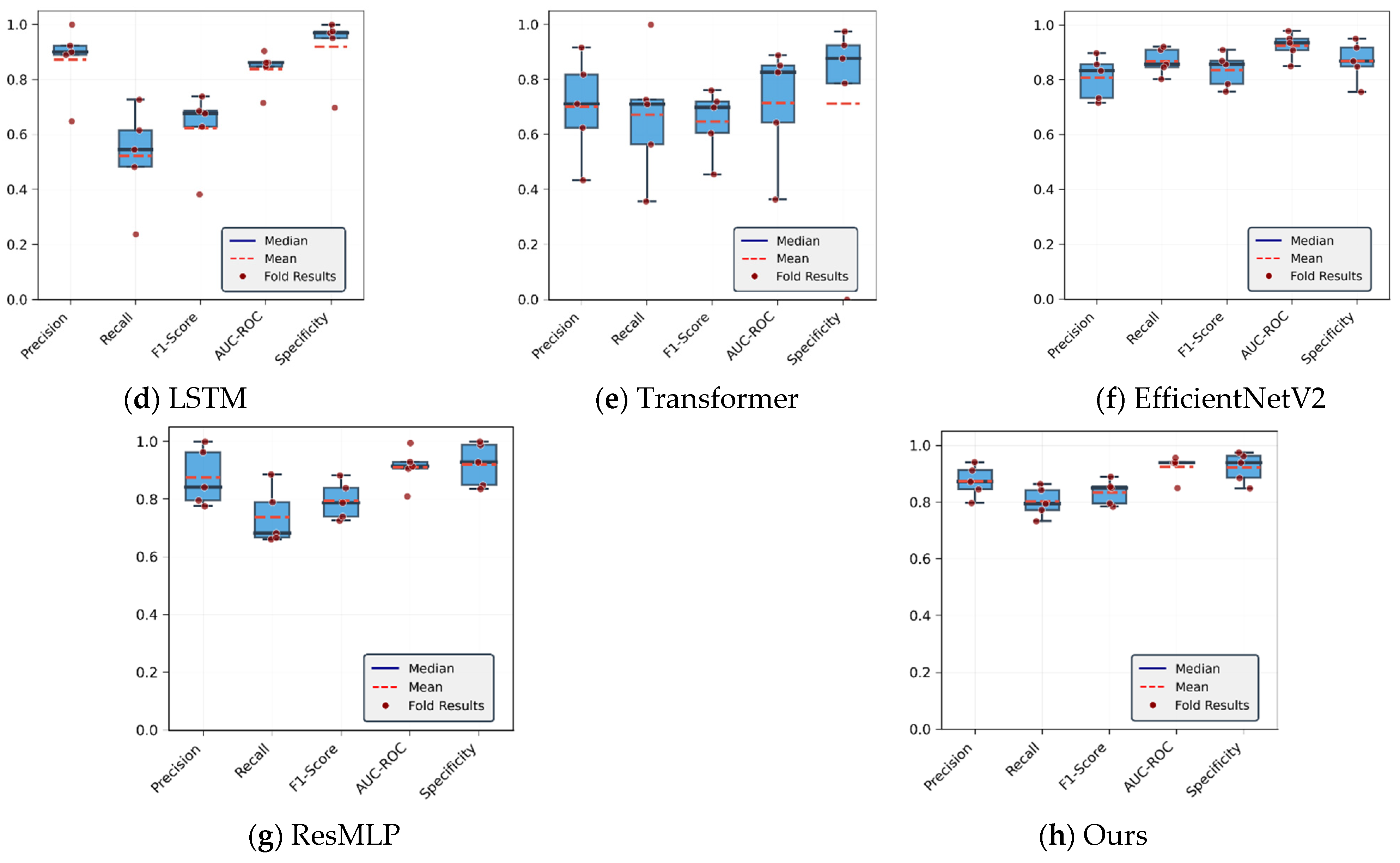
The results presented in Table 3 and Table 4, along with the box plots in Figure 6 and Figure 7, indicate that all three machine learning algorithms performed better on the AP CoP trajectory than on the ML CoP trajectory. This suggests that the AP direction plantar pressure center trajectories are more suitable for hemiplegic gait recognition and possess greater potential clinical diagnostic value.

4.1.2. Analysis of CoP Trajectory Recognition Results Using Deep Learning Methods

In this study, five deep learning methods were employed to recognize hemiplegic gait based on plantar pressure center trajectories, including the LSTM, transformer, EfficientNetV2, ResMLP, and proposed temporal–frequency domain interaction network (TFDI-Net) methods. Their performance was evaluated using five-fold cross-validation on plantar pressure data from 48 participants (29 healthy individuals and 19 hemiplegic patients). The results revealed significant performance differences among the models. Overall, the proposed TFDI-Net achieved the best performance, followed by ResMLP. EfficientNetV2 ranked third, with the LSTM and transformer methods performing slightly worse in sequence.
As a deep learning model specifically designed for sequence data, LSTM demonstrated the fourth performance in this study, following EfficientNetV2. It achieved an accuracy rate of 87.66% and an AUC-ROC of 93.6%, indicating its effectiveness in capturing the temporal dependencies within plantar pressure center trajectories. The gated architecture of LSTM enables it to learn long-term dependency patterns in gait signals, which is particularly valuable for identifying abnormal temporal characteristics associated with hemiplegic gait. However, the recall of LSTM was relatively low (77.13%), suggesting a certain risk of missed diagnoses when identifying hemiplegic patients. This limitation may stem from LSTM’s reliance solely on temporal features, without incorporating frequency domain information, which could reduce its effectiveness in recognizing certain types of hemiplegic gait patterns.
The transformer model, with its self-attention mechanism, is theoretically capable of capturing dependencies between any positions within a sequence, offering stronger modeling capacity than LSTM. However, in this study, the transformer achieved slightly lower performance, with an accuracy of 85.47%, compared to LSTM. This may be attributed to the fact that transformer architectures typically require large-scale datasets to effectively train their complex attention mechanisms, whereas the number of subjects in this study (48 participants) may not have been sufficient to fully exploit the model’s potential. As shown in the box plots, the transformer exhibited relatively high variability across evaluation metrics, particularly in recall, indicating that its performance stability remains suboptimal in this small-sample setting.
The recognition performance of ResMLP can be explained by its architectural design. The model adopts a patch embedding mechanism that divides the CoP spectrogram into patches, followed by 12 MLP-based residual blocks for feature learning. Its high specificity (92.09%) can be attributed to the regularity of plantar pressure control patterns in healthy individuals. These dynamic patterns are consistent within each patch and can be effectively captured through deep feature abstraction, resulting in clearly clustered feature distributions. However, the model’s recall is relatively low (73.98%), which may be due to the use of a global average pooling strategy that tends to dilute localized abnormal signals from hemiplegic patients—especially in cases of mild hemiplegia, where abnormalities typically occur only during specific phases of the gait cycle. Nevertheless, the model achieved an excellent AUC-ROC score (93.24%), indicating that the 384-dimensional embedding space it constructs is highly expressive and enables clear linear separability between hemiplegic and healthy samples in the high-dimensional representation space.
EfficientNetV2 exhibited moderate performance in the analysis of anterior–posterior (AP) CoP trajectories. Specifically, the model achieved an accuracy rate of 85.88%, a precision rate of 83.01%, an F1-score of 82.18%, and an AUC-ROC of 93.12%, slightly underperforming compared to ResMLP. Notably, its specificity surpassed that of ResMLP, reaching 81.36%. However, this still implies that approximately 18.64% of healthy individuals were misclassified as hemiplegic patients—an outcome that remains unacceptable in clinical applications. The core module of EfficientNetV2 is the mobile inverted bottleneck convolution (MBConv) block, which may struggle to capture critical features when extracting information from spectrograms. The use of depthwise separable convolutions and channel attention mechanisms is better suited for capturing spatial correlations, and may require further structural optimization to effectively extract meaningful frequency domain features. In the AP direction CoP trajectory analysis, crucial information lies in dynamic temporal patterns and long-range dependencies within the time series. However, EfficientNetV2 focuses more on local feature extraction and inter-channel weighting, which limits its ability to effectively model the temporal dynamics essential for accurate gait recognition.
The proposed TFDI-Net achieved the highest hemiplegic gait recognition accuracy on the AP CoP trajectory dataset, which can be attributed to several key architectural designs. First, the temporal feature extraction module utilizes only three 1D convolutional layers to capture local temporal dependencies. Then, frequency domain features are extracted via Fourier transform and further processed using three additional convolutional layers. Finally, the temporal and frequency features are integrated through a domain interaction mechanism, resulting in more discriminative representations. An analysis of the five-fold cross-validation box plots reveals that TFDI-Net demonstrates excellent stability and generalization capability. The precision metric is consistently concentrated within the 0.95–1.00 range, indicating high consistency and low variance. The AUC-ROC values remain stably within the 0.95–1.00 range as well, reflecting the model’s strong discriminative power across different data splits. The specificity metric also performs remarkably well, with all folds exceeding 0.95. Although the recall metric shows some variability (ranging from 0.75 to 0.95), the overall performance still surpasses that of the other models.
The performance of both machine learning and deep learning methods on AP and ML CoP trajectories suggests that AP direction CoP data hold greater clinical diagnostic value. Moreover, deep learning models do not rely on handcrafted feature extraction, and with the integration of frequency domain information, can achieve superior performance. These findings indicate that deep learning approaches based on temporal–frequency feature fusion offer promising potential for the clinical application of hemiplegic gait recognition.

4.2. Ablation Experiment

To evaluate the contribution of temporal, frequency, and temporal–frequency domain features to hemiplegic gait recognition, ablation experiments were conducted on the temporal convolution module, frequency convolution module, and temporal–frequency interaction fusion module, with the results shown in Table 5. First, by removing the frequency domain feature module from the proposed TFDI-Net model, the baseline performance using only temporal features was obtained. When only the frequency domain feature module was retained, the performance in terms of the F1-score and recall outperformed the results of the temporal feature module. This indicates that models trained with frequency domain features are better at capturing subtle pattern differences, especially those that are not prominent in the time domain but are significant in the frequency domain, thereby reducing the incidence of missed diagnoses.
The accuracy, F1-score, and recall improved after directly merging temporal and frequency features, compared to using only temporal or frequency features individually. This indicates that the fused features provide a richer decision boundary in the high-dimensional feature space. Samples that were difficult to distinguish in a single feature domain were effectively separated in the fused feature space. When temporal and frequency features were further integrated through interaction, the accuracy, F1-score, and recall improved again, suggesting the presence of temporal–frequency coupling features in the CoP trajectory. This nonlinear synergistic effect not only validates the multi-scale dynamic characteristics of the balance control system but also provides an important technical pathway for developing more accurate models for balance function assessments.

4.3. Computational Efficiency

We not only compared the computational efficiency of our method with existing approaches such as SVM, RF, and LSTM, but also with XGBoost, transformer, ResMLP, and EfficientNetV2 methods. The results are presented in Table 6.
Traditional machine learning models are typically trained on CPUs, so only the training time can be reasonably measured; all other metrics are denoted by ‘-‘. Moreover, their parameter counts and model sizes are significantly smaller than those of deep learning models, making direct comparisons less meaningful. Compared with models such as LSTM, transformer, ResMLP, and EfficientNetV2, TFDI-Net achieved competitive performance results, ranking second only to LSTM across all evaluation metrics. This demonstrates its strong potential for real-world clinical deployment.

5. Conclusions

This study proposes a hemiplegic gait recognition method based on temporal–frequency feature interaction, namely the temporal–frequency domain interaction network (TFDI-Net). Comparative experiments with traditional machine learning methods and recent deep learning models validated the potential and effectiveness of temporal–frequency domain fusion in hemiplegic gait recognition. In addition, ablation studies further revealed the existence of temporal–frequency coupling features within the CoP trajectory and demonstrated that feature fusion can effectively improve the recognition performance.
The current dataset consists mainly of healthy individuals and a limited number of hemiplegic patients. Due to safety concerns during data collection, only data from mildly hemiplegic patients were included, which restricts the model’s generalizability to broader pathological gait scenarios. Therefore, further validation on more diverse and representative datasets is required. Future work will focus on collecting plantar pressure data from patients with varying degrees of hemiplegia to optimize the algorithm, and integrating it into an automated gait assessment system based on plantar pressure, with the aim of improving its robustness and clinical applicability.

Author Contributions

Conceptualization, Z.M. and L.M.; methodology, L.M.; software, L.M.; resources, Z.M.; data curation, L.M.; writing—original draft preparation, L.M.; writing—review and editing, Z.M. and L.M.; visualization, L.M.; supervision, Z.M.; project administration, Z.M.; funding acquisition, Z.M. All authors have read and agreed to the published version of the manuscript.

Funding

This work was partially supported by Key R&D Support Project 2021-YF05–02175-SN of the Chengdu Science and Technology Bureau, the Key Project 2023YFG0271 of the Science and Technology Department of Sichuan Province.

Institutional Review Board Statement

The study was conducted in accordance with the Declaration of Helsinki, and approved by the Academic Review Committee of College of Computer Science and Cybersecurity, Chengdu University of Technology for studies involving humans (REF. NO. 2024001).

Informed Consent Statement

Informed consent was obtained from all subjects involved in the study.

Data Availability Statement

The data are not publicly available due to privacy and ethical restrictions.

Acknowledgments

We would like to thank Zhi Li and Nan Jiang for their assistance in recruiting participants, including both patients and healthy controls, for this study.

Conflicts of Interest

The authors declare no conflicts of interest.

References

  1. Cai, G.; Xu, J.; Zhang, C.; Jiang, J.; Chen, G.; Chen, J.; Liu, Q.; Xu, G.; Lan, Y. Identifying Biomarkers Related to Motor Function in Chronic Stroke: A fNIRS and TMS Study. CNS Neurosci. Ther. 2024, 30, e14889. [Google Scholar] [CrossRef] [PubMed]
  2. Qin, S.; Gao, D.; Chen, X.; Ning, S.; Liu, Z.; Li, P. Analysis of Motor Functions of Hemiplegic Patients Based on Dual-Mode Signal Fusion. IEEE Sens. J. 2024, 24, 32694–32706. [Google Scholar] [CrossRef]
  3. Hulleck, A.A.; Menoth Mohan, D.; Abdallah, N.; El Rich, M.; Khalaf, K. Present and Future of Gait Assessment in Clinical Practice: Towards the Application of Novel Trends and Technologies. Front. Med. Technol. 2022, 4, 901331. [Google Scholar] [CrossRef] [PubMed]
  4. Xie, Z.; Xie, L. Gait Feature Construction and Selection Based on Plantar Pressure Insole. In Proceedings of the 2023 5th International Academic Exchange Conference on Science and Technology Innovation (IAECST), Guangzhou, China, 8–10 December 2023; pp. 982–987. [Google Scholar]
  5. Potluri, S.; Ravuri, S.; Diedrich, C.; Schega, L. Deep Learning Based Gait Abnormality Detection Using Wearable Sensor System. In Proceedings of the 2019 41st Annual International Conference of the IEEE Engineering in Medicine and Biology Society (EMBC), Berlin, Germany, 23–27 July 2019; pp. 3613–3619. [Google Scholar]
  6. Hayashi, Y.; Yasuda, K.; Kitaji, Y.; Harashima, H.; Iwata, H. A Haptic-Based Perception-Empathy Biofeedback Device That Supplements Foot Pressure Pattern during Gait in Stroke Patients. In Proceedings of the 2019 IEEE/SICE International Symposium on System Integration (SII), Paris, France, 14–16 January 2019; pp. 124–128. [Google Scholar]
  7. LeMoyne, R.; Kerr, W.; Mastroianni, T.; Hessel, A. Implementation of Machine Learning for Classifying Hemiplegic Gait Disparity through Use of a Force Plate. In Proceedings of the 2014 13th International Conference on Machine Learning and Applications, Detroit, MI, USA, 3–6 December 2014; pp. 379–382. [Google Scholar]
  8. Cui, C.; Bian, G.-B.; Hou, Z.-G.; Zhao, J.; Su, G.; Zhou, H.; Peng, L.; Wang, W. Simultaneous Recognition and Assessment of Post-Stroke Hemiparetic Gait by Fusing Kinematic, Kinetic, and Electrophysiological Data. IEEE Trans. Neural Syst. Rehabil. Eng. 2018, 26, 856–864. [Google Scholar] [CrossRef] [PubMed]
  9. Liu, S.; Yu, H.; Wang, Z.; Dai, P. Correlation Analysis of Balance Function with Plantar Pressure Distribution and Gait Parameters in Patients with Cerebral Infarction in the Basal Ganglia Region. Front. Neurosci. 2023, 17, 1099843. [Google Scholar] [CrossRef] [PubMed]
  10. Sanghan, S.; Chatpun, S.; Leelasamran, W. Gait Characterizations under Dynamic Load during Walking in Hemiplegic Patients. In Proceedings of the 4th 2011 Biomedical Engineering International Conference, Chiang Mai, Thailand, 29–31 January 2012; pp. 22–25. [Google Scholar]
  11. Rastegarpanah, A.; Scone, T.; Saadat, M.; Rastegarpanah, M.; Taylor, S.J.; Sadeghein, N. Targeting Effect on Gait Parameters in Healthy Individuals and Post-Stroke Hemiparetic Individuals. J. Rehabil. Assist. Technol. Eng. 2018, 5, 2055668318766710. [Google Scholar] [CrossRef] [PubMed]
  12. Kokolevich, Z.M.; Biros, E.; Tirosh, O.; Reznik, J.E. Distinct Ground Reaction Forces in Gait between the Paretic and Non-Paretic Leg of Stroke Patients: A Paradigm for Innovative Physiotherapy Intervention. Healthcare 2021, 9, 1542. [Google Scholar] [CrossRef] [PubMed]
  13. Park, C.; Woo, Y.; Won, J.; Kim, S. Immediate Effects of Insoles Applied to the Sound Side Lower Extremity of Patients with Chronic Hemiplegia during Walking. Restor. Neurol. Neurosci. 2024, 42, 167–177. [Google Scholar] [CrossRef] [PubMed]
  14. Kim, C.-H.; Chu, H.; Kang, G.-H.; Sung, K.-K.; Kang, D.G.; Lee, H.S.; Lee, S. Difference in Gait Recovery Rate of Hemiparetic Stroke Patients According to Paralyzed Side: A Cross-Sectional Study Based on a Retrospective Chart Review. Medicine 2019, 98, e18023. [Google Scholar] [CrossRef] [PubMed]
  15. Cortes, C.; Vapnik, V. Support-Vector Networks. Mach. Learn. 1995, 20, 273–297. [Google Scholar] [CrossRef]
  16. Breiman, L. Random Forests. Mach. Learn. 2001, 45, 5–32. [Google Scholar] [CrossRef]
  17. Chen, T.; Guestrin, C. XGBoost: A Scalable Tree Boosting System. In Proceedings of the 22nd ACM SIGKDD International Conference on Knowledge Discovery and Data Mining, San Francisco, CA, USA, 13–17 August 2016; pp. 785–794. [Google Scholar]
  18. Tan, M.; Le, Q. EfficientNetV2: Smaller Models and Faster Training. In Proceedings of the Proceedings of the 38th International Conference on Machine Learning, PMLR, Online, 18–24 July 2021; pp. 10096–10106. [Google Scholar]
  19. Vaswani, A.; Shazeer, N.; Parmar, N.; Uszkoreit, J.; Jones, L.; Gomez, A.N.; Kaiser, L.; Polosukhin, I. Attention Is All You Need. arXiv 2017, arXiv:1706.03762v7. [Google Scholar]
  20. Touvron, H.; Bojanowski, P.; Caron, M.; Cord, M.; El-Nouby, A.; Grave, E.; Izacard, G.; Joulin, A.; Synnaeve, G.; Verbeek, J.; et al. ResMLP: Feedforward Networks for Image Classification With Data-Efficient Training. IEEE Trans. Pattern Anal. Mach. Intell. 2023, 45, 5314–5321. [Google Scholar] [CrossRef] [PubMed]
  21. Hochreiter, S.; Schmidhuber, J. Long Short-Term Memory. Neural Comput. 1997, 9, 1735–1780. [Google Scholar] [CrossRef] [PubMed]
  22. Macdonald, E.; Larracy, R.; Phinyomark, A.; Scheme, E. Underfoot Pressure-Based Left and Right Foot Classification Algorithms: The Impact of Footwear. IEEE Access 2023, 11, 137937–137947. [Google Scholar] [CrossRef]
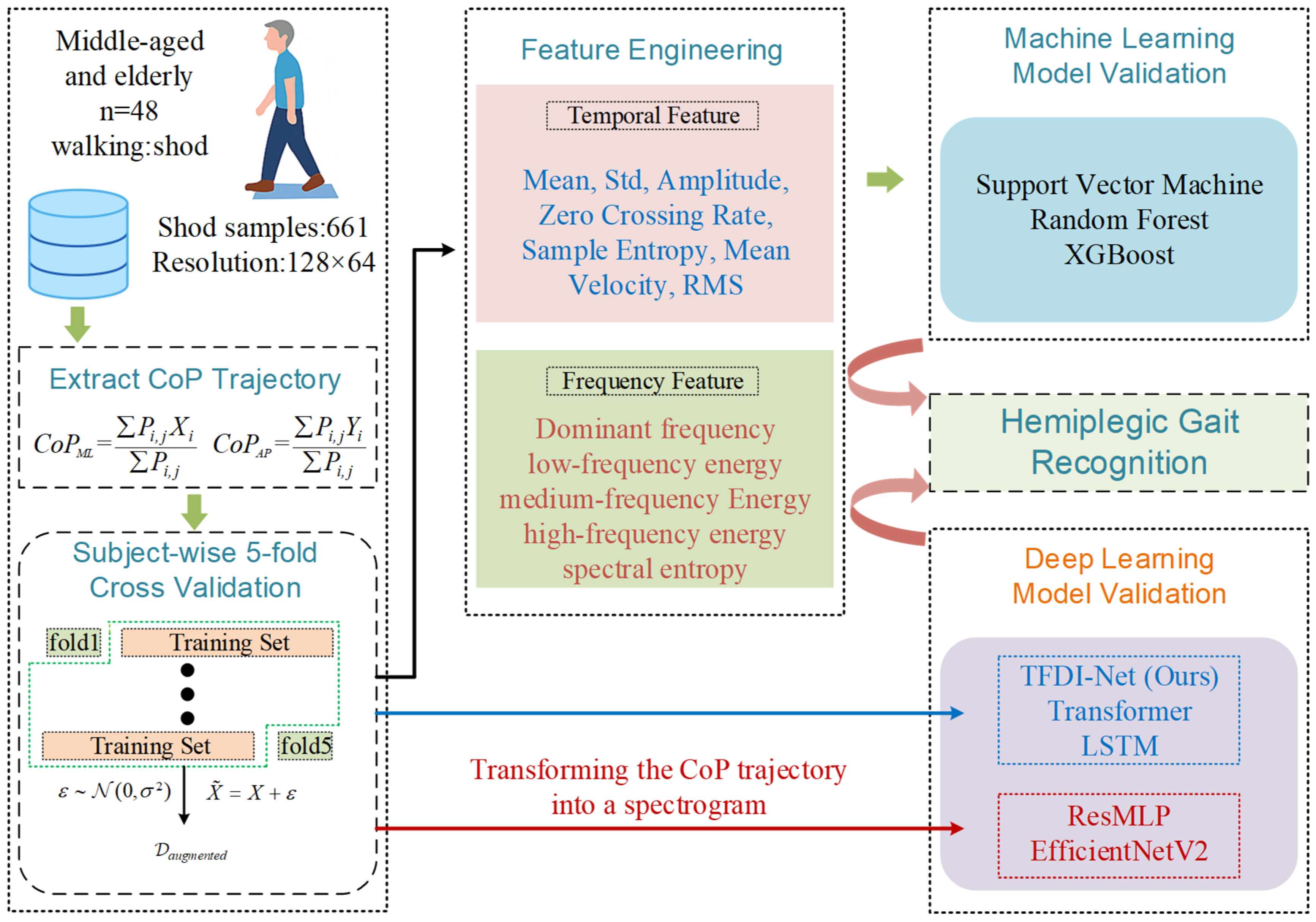
Figure 1. Workflow of the proposed study.
Computers 14 00334 g001
Figure 2. Experimental data collection.
Computers 14 00334 g002
Figure 3. Visualization of CoP trajectories in the ML direction.
Computers 14 00334 g003
Figure 4. Visualization of CoP trajectories in the AP direction.
Computers 14 00334 g004
Figure 5. TFDI-Net network structure.
Computers 14 00334 g005
Figure 6. Box plot of five-fold cross-validation on AP CoP.
Computers 14 00334 g006
Figure 7. Box plot of five-fold cross-validation on ML CoP.
Computers 14 00334 g007aComputers 14 00334 g007b
Table 1. Demographic information of middle-aged and elderly participants.
HealthyHemiplegicTotal
Age58.9 ± 8.961.6 ± 10.960.0 ± 9.8
Sex8/2116/524/26
Height (cm)164 ± 14161 ± 11164 ± 14
Weight (kg)65 ± 2265 ± 1765 ± 22
Shoe Size (EU)39 ± 339 ± 339 ± 3
Hemiplegic Side0/011/1011/10
Table 2. TFDI-Net structure settings.
ModuleLayer NameInput ChannelsOutput ChannelsKernel SizeActivationPool
time featureconv1500645ReLUMaxpool
conv2641285ReLUMaxpool
conv31282565ReLUMaxpool
fft-----
freq featureconv12323ReLUMaxpool
conv232643ReLUMaxpool
conv3641283ReLUMaxpool
time2freq magconv256641ReLU-
conv642561Segmoid-
freq2time magconv128641ReLU-
conv641281Segmoid-
freq_enhancementconv384641ReLU-
conv643841Tanh-
time2freq correlationLinear138464-ReLU-
Linear2641-Sigmoid-
feature
fusion
conv512621ReLU-
conv625121Sigmoid-
adaptive pool-62---
fc1 --ReLU-
dropout-----
fc2-----
Table 3. Hemiplegic gait recognition results based on AP direction CoP trajectories.
ModelAccuracyPrecisionF1-ScoreAUC-ROCSpecificityRecall
SVM86.9989.2382.7692.7591.777.17
RF84.8183.7380.4891.787.977.48
XGBoost84.7584.8179.6590.4489.5375.05
LSTM87.6690.4683.2693.6092.8577.13
Transformer85.4788.7879.6092.3192.3772.15
EfficientNetV285.8883.0182.1893.1287.5681.36
ResMLP86.0789.5681.0393.2492.0973.98
Ours89.8889.3987.3694.991.9385.42
Table 4. Hemiplegic gait recognition results based on ML direction CoP trajectories.
ModelAccuracyPrecisionF1-ScoreAUC-ROCSpecificityRecall
SVM81.1383.0273.2186.3389.2765.48
RF79.2476.4271.1286.5685.8266.51
XGBoost79.9877.7972.587.5985.9867.88
LSTM77.8587.2165.2683.7691.8452.14
Transformer73.2972.7571.8174.3971.8770.89
EfficientNetV286.9180.7583.6392.4486.8186.73
ResMLP85.5487.5180.0191.079273.7
Ours88.6188.7385.0691.9792.6581.71
Table 5. Results of ablation experiments.
TFFusionAccuracyPrecisionF1-ScoreAUC-ROCSpecificityRecall
88.8189.7785.1495.1692.7080.97
88.5688.5185.7494.1690.7283.13
89.488.2486.7494.9790.8285.29
89.8889.3987.3694.991.9385.42
’T’ represents the temporal feature extraction module, ‘F’ represents the frequency domain feature extraction module, and ‘fusion’ represents the temporal–frequency interaction module.
Table 6. Computational efficiency of machine learning and deep learning models.
ModelParameters (M)Size (MB)Training Time (s)Inference Time (ms)
SVM--35-
RF--59-
XGBoost--25-
LSTM0.170.6955.40.5
Transformer31.962.76062
EfficientNetV220.378.08105513.48
ResMLP14.3654.778743.35
Ours12.7748.731952.3
Disclaimer/Publisher’s Note: The statements, opinions and data contained in all publications are solely those of the individual author(s) and contributor(s) and not of MDPI and/or the editor(s). MDPI and/or the editor(s) disclaim responsibility for any injury to people or property resulting from any ideas, methods, instructions or products referred to in the content.