Parallel Sort Implementation and Evaluation in a Dataflow-Based Polymorphic Computing Architecture

Abstract

This work presents two variants of an odd–even sort algorithm that are implemented in a dataflow-based polymorphic computing architecture. The two odd–even sort algorithms are the “fully unrolled” variant and the “compact” variant. They are used as test kernels to evaluate the polymorphic computing architecture. Incidentally, these two odd–even sort algorithm variants can be readily adapted to ASIC (Application-Specific Integrated Circuit) and FPGA (Field Programmable Gate Array) designs. Additionally, two methods of placing the sort algorithms’ instructions in different configurations of the polymorphic computing architecture to achieve performance gains are furnished: a genetic-algorithm-based instruction placement method and a deterministic instruction placement method. Finally, a comparative study of the odd–even sort algorithm in several configurations of the polymorphic computing architecture is presented. The results show that scaling up the number of processing cores in the polymorphic architecture to the maximum amount of instantaneously exploitable parallelism improves the speed of the sort algorithms. Additionally, the sort algorithms that were placed in the polymorphic computing architecture configurations by the genetic instruction placement algorithm generally performed better than when they were placed by the deterministic instruction placement algorithm.

1. Introduction

Polymorphic computing [1] is an emerging area of study where the architecture of a computing system (as opposed to the software) is changed just before runtime or during runtime to achieve some kind of benefit (for instance, executing algorithms in a parallel manner to increase their speed of execution). Essentially, the runtime computing architectural arrangement is dynamic. Examples of polymorphic systems are TRIPS [2,3,4,5,6], Raw [7,8,9,10], MONARCH [11,12,13], MOLEN [14], and ρ-VEX [15].

Recently, a new polymorphic computing architecture based on a fabric of dataflow processors was introduced in [16,17,18,19]. (In this context, “dataflow” is an instruction set architecture [20,21,22] that is an alternative to CISC (Complex Instruction Set Computer) [23] and RISC (Reduced Instruction Set Computer) [24,25,26] instruction set architectures.) The next research steps are to adapt traditional algorithms to this architecture to evaluate both the architecture and the algorithm simultaneously. This work is one step in the greater effort to evaluate and draw conclusions about the architecture.

The primary purpose of this work is to evaluate the polymorphic computing architecture using an odd–even sort algorithm (a parallelizable sort algorithm related to bubble sort). In this case, an odd–even sort algorithm was chosen to be evaluated in the architecture due to it representing an ubiquitous category of algorithms (i.e., sorting), its large amount of available fine-grained parallel execution opportunities, and its relative algorithmic simplicity compared to other sorts.

The secondary purpose of this work is to provide a new description of the odd–even sort that describes the internal sort lattice and the strategy to compact (reduce) the size of the algorithm.

The contributions of this work are

• A presentation of two variants of a parallel odd–even sort algorithm expressed in the dataflow-based polymorphic computing architecture’s instruction set (which have applications to ASIC-based or FPGA-based systems outside of this work):

  (a)

  A “fully unrolled” parallel odd–even sort;

  (b)

  A “compact” parallel odd–even sort.

• A comparative study of the odd–even sort performance in a number of two-dimensional variants of the polymorphic computing architecture.
• Two methods for placing the sort algorithms’ instructions in the various polymorphic architecture variants to achieve performance gains over single-processor instances:

  (a)

  A genetic-algorithm-based placement method;

  (b)

  A deterministic instruction placement method.

To fulfill the purposes of this work, the article is structured into

• An “Introduction” that lays out the purposes and contributions of this work (this section);
• A “Background” section that goes over the basics of the polymorphic computing architecture;
• A “Materials and Methods” section, which is further composed of

  –

  A section called “Odd–Even Sort Algorithms (closely related to Bubble Sort)” that details the motivations and constructions of the “fully unrolled” and “compact” odd–even sort algorithm variants;

  –

  A section called “Evaluation Methods” that describes the experiments;

• A “Results” section that presents the measurement metrics and the results themselves;
• A “Results Discussion” section that examines the experimental results;
• A “Conclusions” section.

Note that the Appendix A listed after the conclusion detail where to locate the Python 3 scripts that were used to generate the result graphs and where to locate visualization videos of the internal behavior of select experiments. The data shown in the results section are embedded in the Python scripts.

2. Background

In previous works, a polymorphic architecture based on a dataflow processor core was presented [16,17,18]. In essence, this is a processor core in which programs can be written in a manner that allows fine-grained parallelism at the instruction level to be expressed/exploited. Further, by tiling multiple instances of these processor cores together, a single program can have its instructions independently assigned (“draped”) across the processors to increase the amount of parallel execution units that are available to the program at any one time. The different “drapings” of a program over the cores present different computer architectures from the viewpoint of that program. Essentially, the ability to change these “drapings” of a program over the cores establishes the computer architecture as a polymorphic computing architecture. The polymorphic architecture of this work is the family of arrangements of one or more of these dataflow processors together. The following paragraphs explain the fundamental pieces that enable the polymorphic computing architecture and describe how they are collected together to form the polymorphic computing architecture.

The key enablers of the hardware polymorphism are

• The dataflow instruction design;
• The operation cell.

The dataflow instruction is a logical construct, while the operation cell is a physical construct that holds the dataflow instruction. Together, these provide both specification and implementation of a program’s instruction.

The dataflow instruction fields are shown in Figure 1. The instruction is designed to be both atomic and independent of other instructions. Each instruction can independently execute (“fire”) when its inputs have fully arrived. Essentially, this enables multiple instructions to simultaneously execute. Each instruction is capable of expressing both operations and decisions in a single action. There are two operations available to each instruction that are executed in parallel (Operation X and Operation Y). Additionally, there is decision logic expressed in each instruction (Input Selectors and Look-Up Table) that selects the result of one and only one operation as the sole output of the instruction and determines where that result is routed.

The operation cell is the physical implementation that holds and manages a dataflow instruction. A simplified view of this cell is shown in Figure 2. Essentially, the operation cell holds an instruction, manages its inputs, and determines whether to execute the instruction or forward the inputs to another operation cell.

Operation cells and one or more ALUs (arithmetic logic units) are collected together to form a single dataflow processor core. Each one of these processor cores is capable of executing a full program expressed in the dataflow instruction set. However, one of these processor cores by itself is not polymorphic because only one hardware architecture is presented to a program (i.e., the hardware architecture cannot change around the program).

An interconnected collection of these single dataflow processor cores creates a compute fabric in which a program’s instructions can be migrated around (i.e., “draped”) without changing the program itself. The family of all possible processor counts along with all possible interconnection implementations define the polymorphic computing architecture. Figure 3 shows an example of a program placed in one possible implementation of the polymorphic architecture. A single instruction is only assigned to be executed by one processor core. Operation cells in processors not assigned to execute that instruction forward their inputs to the operation cell that is assigned to execute the processor. Notice that program instructions can be migrated from one core to another if the input forwarding is maintained. A movement of an instruction between cores effectively presents a different configuration of the computing architecture to a program. This ability to migrate instructions (i.e., change the computer architecture that is presented to a program) makes this a polymorphic computing architecture. (Note that a particular arrangement/placement of instructions in the fabric is referred to as a “geometric placement”).

The odd–even sort algorithms that are executed in this work are expressed in diagrams that reflect the underlying instruction set of the dataflow processor cores. See [16,18,19] for further details of the instruction set.

3. Materials and Methods

3.1. Odd–Even Sort Algorithms (Closely Related to Bubble Sort)

Bubble sort is one of the first sort algorithms taught to programmers due to its simplicity. The name is an analogy for the sorting behavior that occurs in a column of intermixed heavy liquid and light gas when exposed to some kind of uniform force (for example, gravity on Earth or apparent centrifugal forces in a centrifuge). When the force acts upon the mixture, the lighter gas will clump together in bubbles and move towards the “top” of the column (i.e., the opposite direction of the force), while the heavier liquid will move towards the “bottom” of the column (i.e., in the direction of the force). The bubbling process appears to stop when the gas and liquid have been completely separated (sorted) at the “top” and “bottom” of the column, respectively. The bubble sort algorithm works in a very similar way on a list by iteratively bubbling smaller values towards one end of a list and larger values toward the other end. Given enough iterations of the algorithm (no more than the number of elements minus one), the list will be sorted in order.

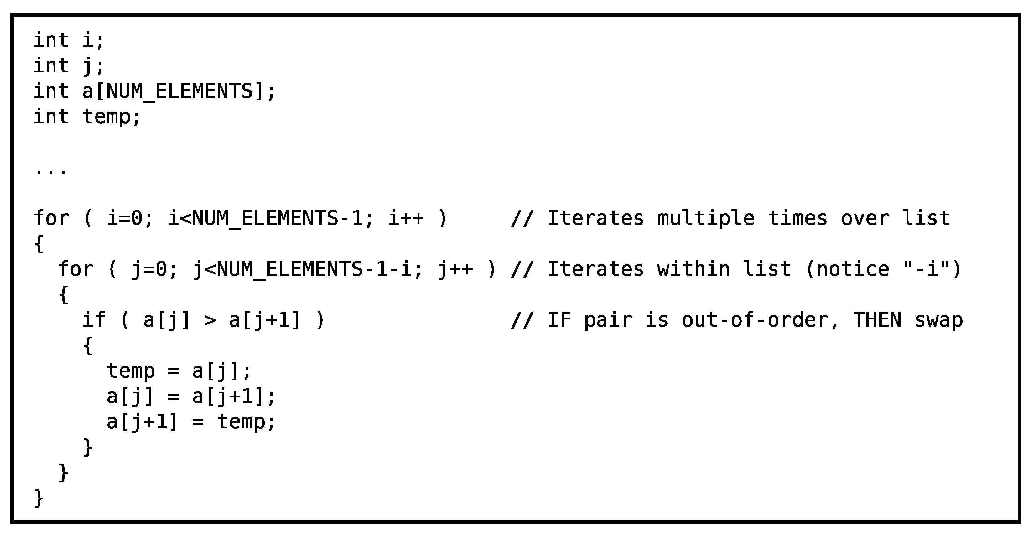
The traditional bubble sort algorithm is expressed algorithmically in Figure 4 [18]. It is composed of an outer loop that iterates over the entire list multiple times and an inner loop that iterates across contiguous element pairs in the list. Essentially, the inner loop implements a sliding window that encompasses two contiguous elements at a time. When the two elements are out-of-order with respect to on another, the elements are swapped. The type of list ordering (i.e., ascending in value, descending in value, etc.) is selected in the “if” condition inside the loops by specifying how one value is greater than another. Overall, the two loops sweep the swap window over the list multiple times. The smaller values appear to “bubble” to one end of the list, while the larger values settle to the other side of the list.

The number of potential swap operations in traditional bubble sort algorithm is

$$swaps=\sum _{j=1}^{N-1}j={\displaystyle \frac{(N-1)\left(N\right)}{2}}={\displaystyle \frac{N^2-N}{2}}$$

(1)

The outer loop of the algorithm is represented in the equation by the summation operation. The j within the summation represents the number of potential swaps in each inner loop. The N represents the number of items in the list. Notice that the equivalent form of the equation says that the number of potential swaps increases by the square of the number of elements in the list.

Figure 5 shows an example of a list of numbers in descending order that is bubble sorted into ascending order [18]. The “bubbles” are shown as circles and the swap window is shown as brackets. The term “pass” refers to the iteration number of single single sweep of the swap window through the entire list (i.e., the index of the outer loop in Figure 4). The term “pair” refers to the index of the left value in the swap window (i.e., the index of the inner loop in Figure 4). Notice that the largest value in a pass of the swap window across the list always ends up in its final sorted list position. In successive passes of the swap window, there is no need to include values that are in their final sorted position, so the algorithm skips these values in successive passes of the swap window.

Unfortunately, the bubble sort algorithm shown in Figure 4 is not parallelizable. Each iteration is dependent on the results of the previous iteration because the swap windows overlap between iterations.

However, the traditional bubble sort algorithm can be rearranged so that a set of swap windows can be executed in parallel at any one time (i.e., they have no dependencies with one another). This rearrangement is called an odd–even sort [27,28,29,30,31,32]. Figure 6 shows a rearranged version of the bubble sort algorithm (i.e., an odd–even sort algorithm) where the iterations of the inner loops can be executed in parallel (i.e., the loops can be “unrolled”).

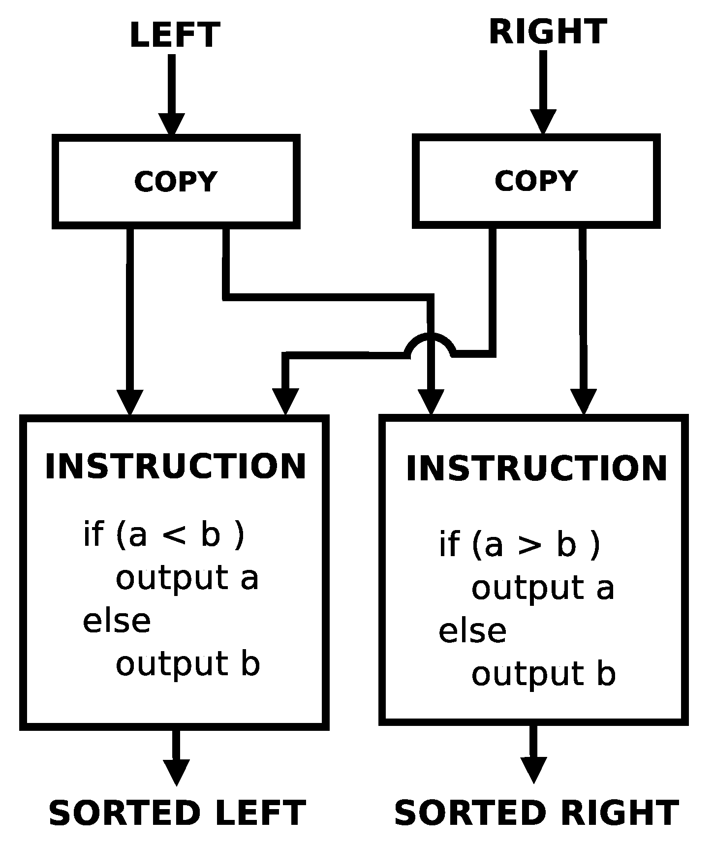
Figure 7 shows the implementation of a single swap in this dataflow processor. It takes 4 instructions to implement. Notice that there are potential parallel execution opportunities within this swap. The left and right branches can potentially execute in parallel. Assuming that both inputs into the swap are available simultaneously, both copy instructions could potentially execute simultaneously in 1 clock cycle, and then both propagate instructions could potentially execute simultaneously in 1 clock cycle. So, in theory, a single swap could complete in 2 clock cycles.

The rearranged algorithm can be fully unrolled into the underlying swap pairs. Figure 8 and Figure 9 show the algorithm fully unrolled along with examples of a worst case list as it progresses along the lattice. Each swap in a row can be executed in parallel with any of the other swaps in a row. Each row corresponds to one of the inner loops in Figure 6. There are two different patterns that emerge in this rearrangement: one when the number of inputs is even and one when the number of inputs is odd.

The even number of inputs pattern of the rearranged algorithm is characterized by N (number of inputs) rows. The even-numbered rows have ${\displaystyle \frac{N}{2}}$ potential swaps. There are ${\displaystyle \frac{N}{2}}$ of these rows. The odd-numbered rows have ${\displaystyle \frac{N}{2}}-1$ potential swaps. There are ${\displaystyle \frac{N}{2}}$ of these rows as well. The number of potential swaps in the rearranged algorithm is given by

$$swap{s}_{even}=\left({\displaystyle \frac{N}{2}}\right)\left({\displaystyle \frac{N}{2}}\right)+\left({\displaystyle \frac{N}{2}}-1\right)\left({\displaystyle \frac{N}{2}}\right)={\displaystyle \frac{N^2-N}{2}}$$

(2)

Notice that this is the same number of potential swaps as the traditional algorithm.

The odd number of inputs pattern of the rearranged algorithm is characterized by N (number of inputs) rows, and each row has ${\displaystyle \frac{N-1}{2}}$ potential swaps. In this case, the number of potential swaps is given by

$$swap{s}_{odd}=\left({\displaystyle \frac{N-1}{2}}\right)N={\displaystyle \frac{N^2-N}{2}}$$

(3)

Notice that the number of swaps in the traditional case (Equation (1)), the rearranged even case (Equation (2)), and the rearranged odd case case (Equation (3)) are identical.

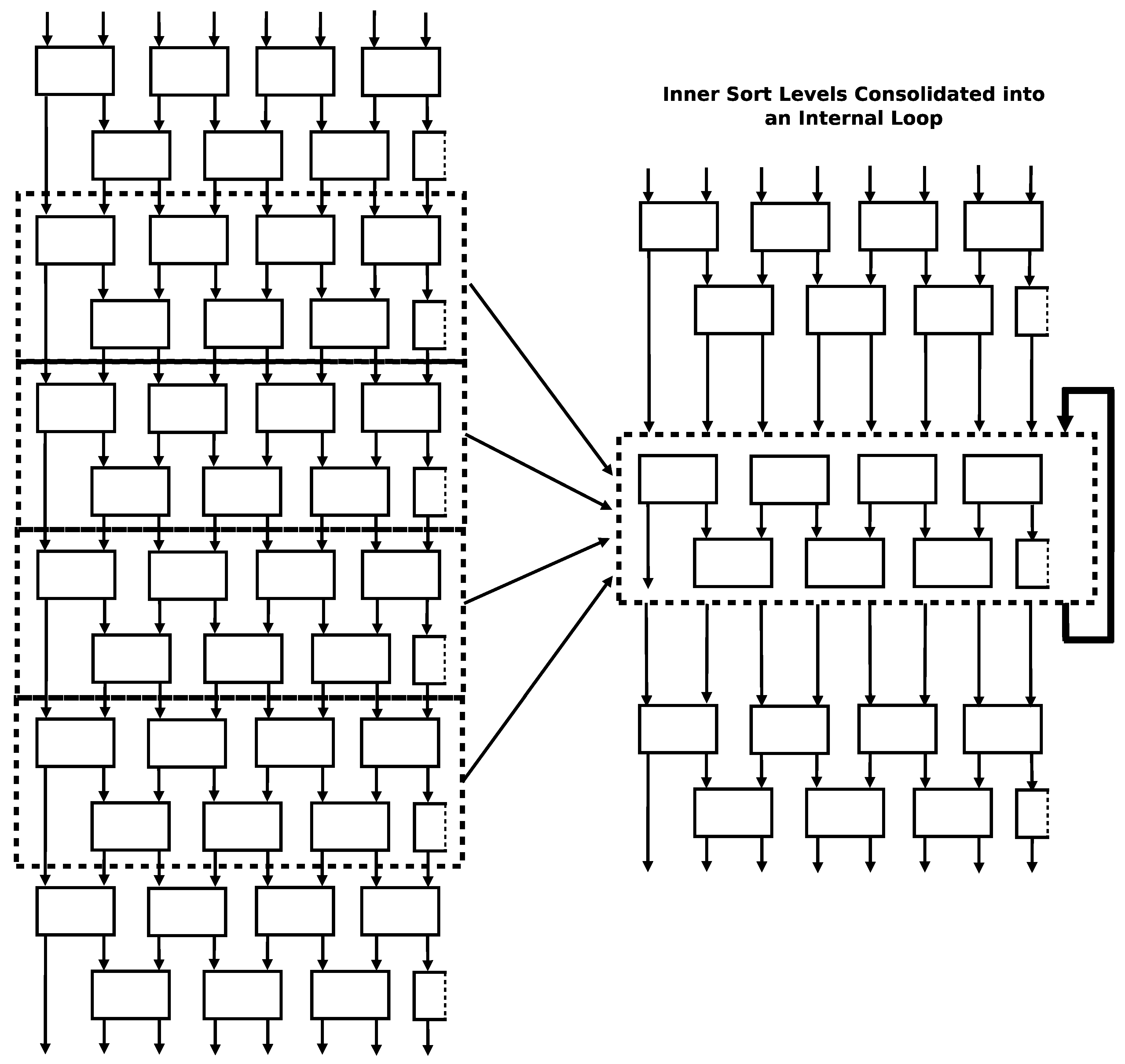
Since the number of swaps in the algorithm rises as a function of the square of the number of inputs, the number of instructions in a fully unrolled version of the rearranged algorithm rises by the square of the number of inputs too. This explosion of instructions can be mitigated by recognizing that every even row/odd row pair in the unrolled structure is identical. These rows can represented as a single entity and placed inside of a loop to reduce the number of actual instructions while still maintaining the ability to execute swaps in parallel. This compaction strategy is visually shown in Figure 10.

Figure 11 shows a diagram of the compact odd–even sort program that is suitable to be implemented in the dataflow processor instruction set of this work [16,18]. It is the odd–even sort algorithm where the inner swap pair rows are nested inside of a loop. The loop mechanism introduces some overall overhead but does not interfere with the amount of simultaneous parallel execution opportunities within the swap pairs in each row. The program implements the first one or two rows independently (one if there is an odd number of inputs and two if there is an even number of inputs), then implements the loop over the inner rows pairs, then implements the last two rows independently. In the figure, the implementation of the first swap row is shown in “Level 0 Sort Level”. The second swap row is shown in “Level 1 Sort Level” (however, this sort row is only implemented in sorts with an even number of inputs). The inner sort rows are shown in “Double Sort Levels Iterator”. The last two sort rows are shown in “Final Double Sort Levels”. The rest of the figure boxes show algorithm flow control. The minimum number of inputs that this program can handle is five. This is the case because there are the same number of swap rows and inputs in the rearranged algorithm. Since this program executes a minimum of five rows (i.e., a minimum of one independently at the beginning, two in a single loop iteration, and two at the end), this means that it can handle a minimum of five inputs. There is no theoretical upper bound on the number of inputs it can handle though. The first and last rows are implemented independently outside of the loop to act as buffers for different execution instances of the sort. The first rows can accept inputs for the next run of the sort while the current run is still being processed in the loop. These support the necessary serialization of multiple runs of the sort. The last row of sorts acts as buffers for the final result of the previous sort and allows the next run of the sort to progress inside of the loop. This allows a new run of the sort to execute concurrently even when the old run has not fully completed yet. (This may happen when the client of the previous sort has not collected all of its results yet).

As an aside: in this work, the odd–even sort is used as a test kernel to evaluate the performance of the polymorphic computing architecture. However, the odd–even sort implementations above can be readily adapted for independent use in FPGAs (Field Programmable Gate Arrays) and ASICs (Application-Specific Integrated Circuits). For instance, Korat, Yadav, and Shah have already independently implemented odd–even sort in an FPGA [31].

3.2. Evaluation Methods

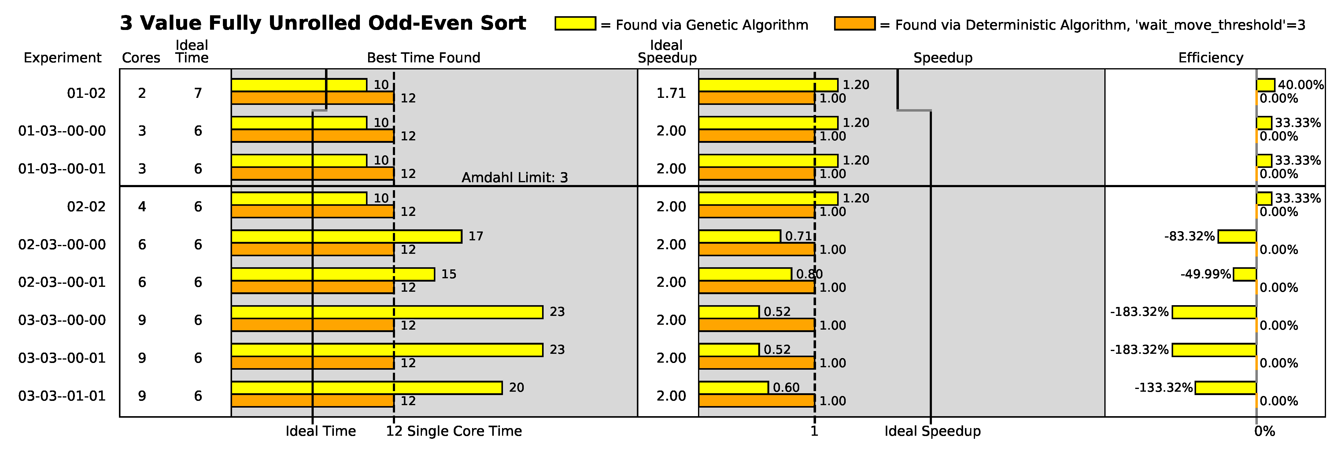
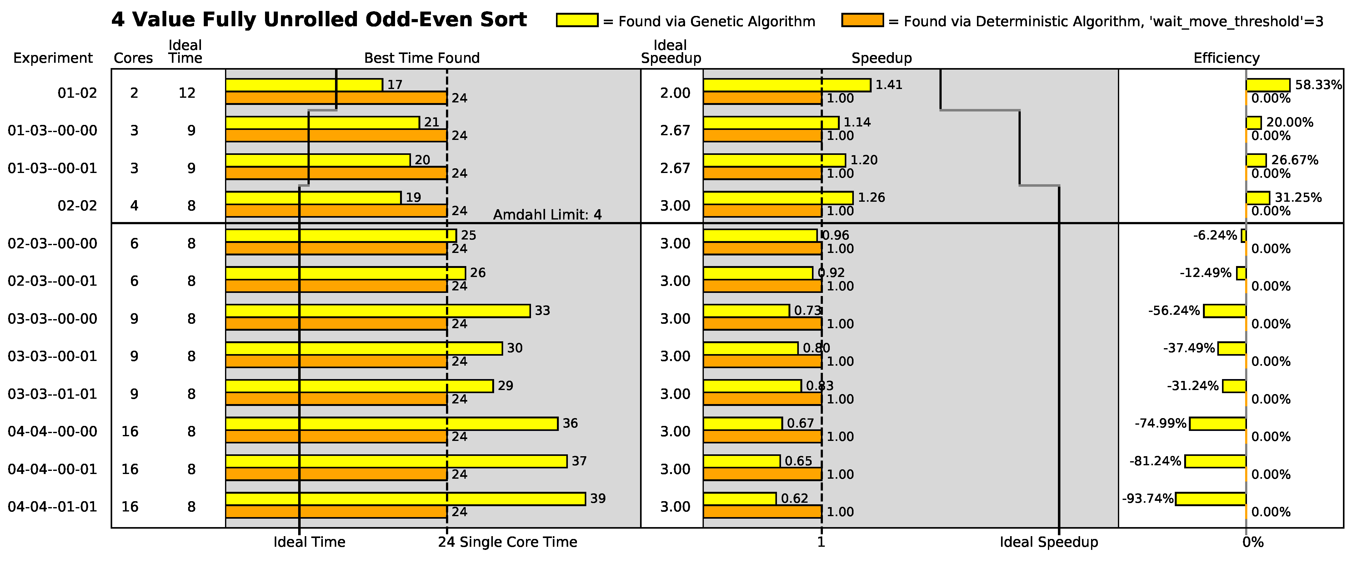
To evaluate the odd–even sort algorithm in this polymorphic computing architecture, five different algorithm variations were each assessed in different geometric configurations of the polymorphic computing architecture. Each assessment was composed of three evaluations performed in a custom clock-accurate computer architecture simulator:

• Evaluation of ideal performance;
• Evaluation of performance of best-found geometric placement from a genetic algorithm;
• Evaluation of performance of best-found geometric placement from a deterministic algorithm.

The five different algorithm variations are shown in

Table 1. Odd–even sort algorithm variants.

Algorithm Variant	Implementation	Instructions
3-Value	Fully Unrolled	12
4-Value	Fully Unrolled	24
5-Value	Compact	76
6-Value	Compact	102
1024-Value	Compact	19,444

. The first two variations are the fully unrolled versions of the algorithm. Each swap operation in the fully unrolled form of the algorithm is given its own unique instructions. The fully unrolled form of the algorithm is potentially the most performance-efficient form of the algorithm because it does not have any instruction control flow overhead outside of the swapping actions themselves. Unfortunately, the number of swaps increases by the square of the number of elements (as indicated by Equations (2) and (3)). As a result, all algorithms that handle lists of size five or larger use the compact form of the algorithm to keep the size of the implementation down. The last variant of the algorithm was chosen to be very large to explore algorithm behavior at a very different scale from the first four variants.

Twelve 2-dimensional geometric configurations of the polymorphic computing architecture were chosen for this study and are shown in

Table 2. Experiment configurations of the polymorphic computing architecture.

Configuration	Number Cores	Rows	Columns	I/O Core Row	I/O Core Column
01-02	2	1	2	0	0
01-03–00-00	3	1	3	0	0
01-03–00-01	3	1	3	0	1
02-02	4	2	2	0	0
02-03–00-00	6	2	3	0	0
02-03–00-01	6	2	3	0	1
03-03–00-00	9	3	3	0	0
03-03–00-01	9	3	3	0	1
03-03–01-01	9	3	3	1	1
04-04–00-00	16	4	4	0	0
04-04–00-01	16	4	4	0	1
04-04–01-01	16	4	4	1	1

. Notice that the configuration name in the table encodes the specific geometric configuration of the polymorphic architecture. The first two numbers of a configuration name encode the number of rows and columns in the configuration. If present, the third and fourth numbers of the configuration name indicate which core served as the sole I/O (input/output) core (i.e., the core where the inputs were injected and the results were gathered). For example, the configuration name “02-03–00-01” means that the polymorphic architecture was a 2-row by 3-column configuration where the core at row 0, column 1 served as the I/O core. When the third and fourth numbers are not present in the configuration name, this means that the location of the I/O core, while physically present, is not a relevant differentiator from other configurations.

All odd–even sort algorithm variations with the exception of the 3-value variation were evaluated in all geometric configurations shown in Table 2. The 3-value algorithm variation was limited to a nine-configuration subset of the twelve configurations. The configurations that were omitted provided more processor cores than there are instructions in the algorithm (i.e., these additional cores would provide no utility to the 3-value algorithm variation).

Ideal performance was measured for each algorithm variant in a clock-cycle-accurate processor simulator. The simulator was configured as a single-core processor with a fixed number of instruction processing units (also called arithmetic logic units or ALUs) that had enough resources to execute all ready-to-execute instructions simultaneously up to the number of available ALUs. Each instruction and transaction was configured to have a latency of one clock cycle. Essentially, the simulator was configured to create a situation where the sole performance bottleneck was the number of instruction execution units (i.e., the effects of array geometry, interprocessor communication latency, and number of separate processors are completely eliminated). Each algorithm was then executed/timed in each processor configuration. Note that the architecture configurations in Table 2 with the same number of cores have the same ideal performance for a given algorithm variant since configuration geometry is ignored by this evaluation.

The genetic search algorithm evaluation and the deterministic search algorithm evaluation were the two methods that were used to evaluate algorithm performance in actual geometric configurations. These search (optimization) techniques were used to find “good” instruction placements of the algorithm in a particular configuration since actual “ideal” instruction placements are not known. For performance evaluations, the choice of “good” instruction placements is extremely important since performance is highly dependent on how the instructions are placed (i.e., “draped”) in a particular array geometry. For instance, best performance will generally occur when the instruction placement mechanism simultaneously minimizes the bottleneck (serial) execution paths to a single core to avoid inter-core communication latencies and maximizes the simultaneous parallelism (time overlap) of inter-core communication and instruction executions to “hide” the time penalties of inter-core communication. Additionally, using two diverse techniques provides a comparative assessment of the quality of the search techniques themselves. (It should be noted that the genetic search algorithm and the deterministic search algorithm currently represent the complete list of instruction placement methods in existence for this polymorphic computing architecture. More instruction placement methods are expected to be developed in the future.)

The genetic search algorithm used to find “good” placements has the parameters found in

Table 3. Genetic search algorithm summary.

Parameter	Value
Population Size	256
Subpopulations	5 (see Table 4)
Generations	Variable (see Table 5)
Children per 2 parents	1
	32 bits multiplied by the number of instructions in
String Size	algorithm (plus an additional 32 bits to account for
	an unused instruction location).
Coding	Each instruction location was coded to a unique
	32-bit processor number.
Crossover Type	Each individual bit has 50% inheritance probability
	from first parent and a 50% inheritance probability
	from the second parent. Bits that are irrelevant to
	the array size are zeroed.
Probability of
Mutation Operations	50%: zero mutations at all
Applied to a new	50%: mutation operator applied
new Individual
Mutation Operator	Individual 8-bit sections of strings are fully
	randomized on byte-aligned boundaries. See Table 5
	for mutation probabilities. The mutation probability
	is independently applied to each 8-bit section.
Fitness Operator	An unsigned 64-bit value where the top 32 bits are
	the number of cores where the individual has at
	least one instruction and the bottom 32 bits are
	the execution time subtracted from 0xFFFF FFFF.
	Essentially, the most significant fitness policy is using
	as many cores as possible. This is meant to drive the
	genetic algorithm to create as many parallel execution
	possibilities as possible (i.e., each additional core
	is another parallel execution possibility). It is also
	meant to encourage the genetic algorithm to hop out of
	local minima in the search space (a well-known issue
	with genetic algorithms). Execution speed is
	rewarded for individuals that have the same core
	utilization count.

,

Table 4. Genetic algorithm subpopulations.

Subpopulation	Size
Top survivors from last generation	12
Descendants of top survivors only	25
Descendants of top survivor and random parent	76
Descendant of two random parents	102
Randomly generated individuals	41

and

Table 5. Genetic search parameters specific to studied algorithm.

Algorithm	Number of Generations	Chance of Individual Byte Mutation
3 Value—Fully Unrolled	1000	1/3
4 Value—Fully Unrolled	1000	1/6
5 Value—Compact	1000	1/19
6 Value—Compact	2000	1/25
1024 Value—Compact	20,000	1/4861

. It is essentially a multi-population evolutionary algorithm based on random changes, where the best-performing individuals are preserved intact from one generation to the next (i.e., an elitist selection policy). The population segments are defined by the types of parents. The different population segments are intended to maintain genetic diversity while still rewarding elitism. A union of two parents produces a single offspring string where each 32-bit value maps an instruction in the algorithm to a processor core in the geometric array. Each bit in an offspring string is randomly selected (at a 50% rate) from the bits in the same position in the parent strings (i.e., one possible bit from each parent). Mutations occur on only 50% of the new offspring in 8-bit “bursts”. The lack of mutations in 50% of the new offspring is intended to encourage the exploration of different combinations of traits in the current population without mutation noise. The “burst” mutations are intended to encourage large changes in individual instruction locations. Fitness is determined first and foremost by the number of cores utilized by the placement. A core utilization is defined as having one or more instructions located in a particular core. For placements utilizing the same number of cores, faster execution speed (i.e., fewer clocks) is rewarded over slower execution speed (i.e., more clocks).

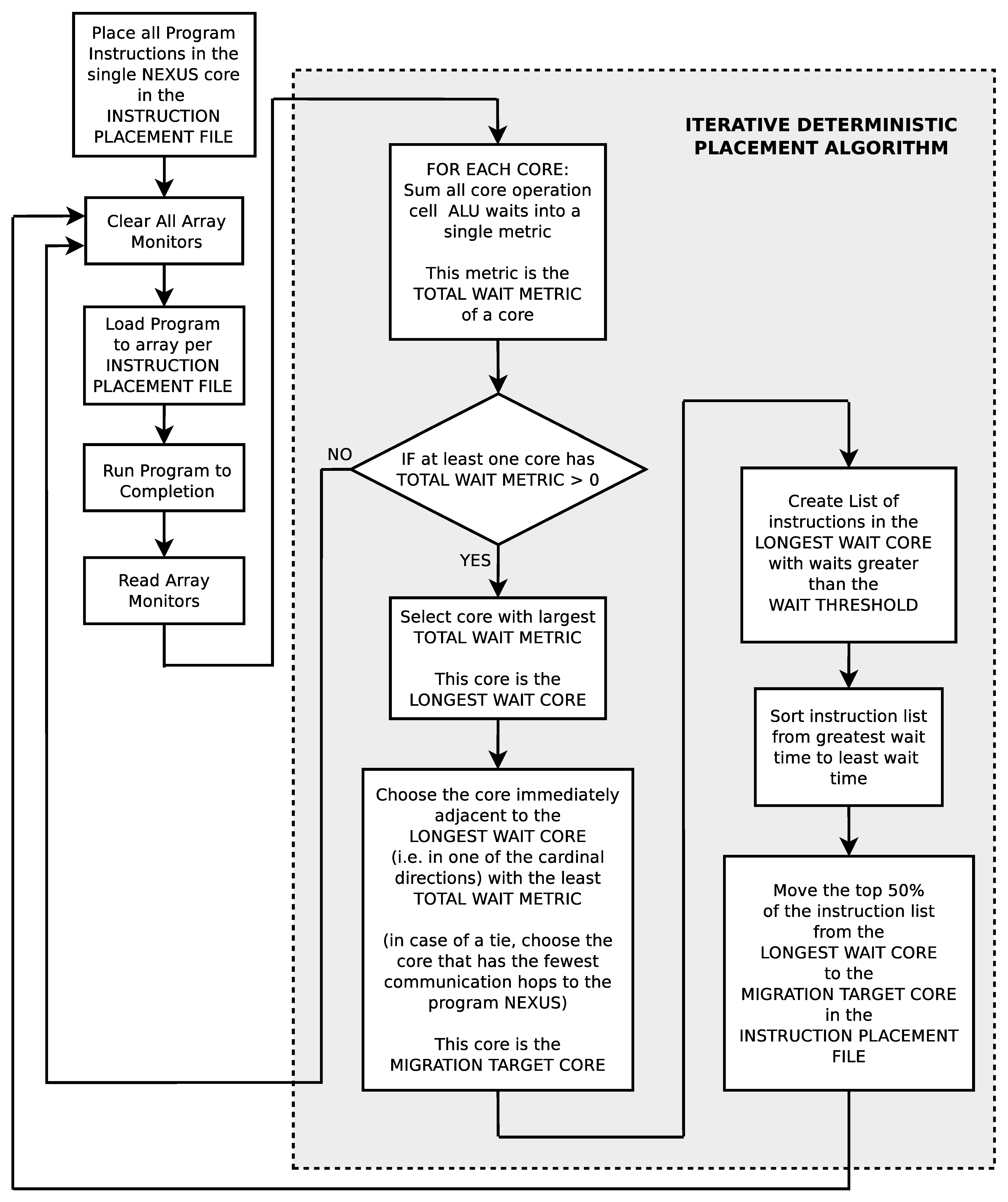
The deterministic search algorithm to find good instruction placements (see Figure 12) is a very different technique than the genetic search algorithm. In this iterative technique, the wait times of each instruction (i.e., the time in clocks between when an instruction became ready to execute and the time it actually was executed) are individually measured on each processor core in the simulator. Essentially, these wait times indicate missed opportunities for instruction execution parallelism. Each iteration of the search essentially runs the current instruction placement in the simulated geometry, measures the individual instruction wait times, selects the processor core with the most cumulative instruction wait times, and moves the selected processor core’s individual instructions that are above a specified wait threshold to the immediately adjacent processor with the least cumulative wait times. The search starts with all instructions located in an individual core and iteratively moves instructions from the most heavily loaded core (as defined by cumulative instruction waiting time) to the least loaded immediately adjacent core. Unlike the genetic algorithm, the deterministic search algorithm does not have a bias to necessarily use all of the processor cores in an array.

4. Results

The results of the odd–even sort algorithm experiments are shown in Figure 13, Figure 14, Figure 15, Figure 16 and Figure 17, with key summaries shown in

Table 6. Odd–even sort algorithm characteristics in polymorphic compute architecture.

Algorithm	Single Core Time	Amdahl Limit
3 Value—Fully Unrolled	12	3
4 Value—Fully Unrolled	24	4
5 Value—Compact	81	6
6 Value—Compact	108	8
1024 Value—Compact	4,188,160	2047

and

Table 7. Best results for odd–even sort algorithms.

Algorithm	Best Cores		Best Time		Best Speedup		Best Efficiency
	Gen	Det	Gen	Det	Gen	Det	Gen	Det
3 Value (U)	2	2	10	12	1.20	1.00	40.0%	0.0%
4 Value (U)	2	2	17	24	1.41	1.00	58.33%	0.0%
5 Value (C)	2	6	47	73	1.72	1.11	87.18%	13.56%
6 Value (C)	2	2	61	95	1.77	1.14	88.68%	24.53%
1024 Value (C)	16	16	801,900	715,171	5.22	5.86	86.32%	88.54%

Gen = Found by Genetic Instruction Placement Algorithm; Det = Found by Deterministic Instruction Placement Algorithm; (U) = Fully Unrolled; (C) = Compact.

. Each figure shows the results of the best found instruction placements for a single algorithm variant across different geometric arrays. Each figure is subdivided into three bar graphs:

• Best time found;
• Speedup;
• Efficiency.

“Best time found” shows the execution time of the best found placement in raw clocks. Shorter times are superior to longer times. “Speedup” compares the performance of the instruction placement compared to the performance of all the instructions operating in a single-processor core. Mathematically, this is expressed as

$$speedu{p}_n={\displaystyle \frac{execution\_tim{e}_1}{execution\_tim{e}_n}}$$

(4)

where $execution\_tim{e}_n$ represents the execution time of the current placement in the current geometry and $execution\_tim{e}_1$ is the execution time when all of the instructions are placed in the same processor core [18]. Larger values are superior to smaller values. “Efficiency” describes how well the current speedup compares to the ideal speedup:

$$efficienc{y}_n={\displaystyle \frac{execution\_tim{e}_1-execution\_tim{e}_n}{execution\_tim{e}_1-ideal\_execution\_tim{e}_n}}$$

(5)

Essentially, this equation expresses a value between 0 and 1 (inclusive) that compares the actual measured improvement of the placement compared to the single-processor execution time versus the ideal execution time compared to the single-processor execution time.

The yellow bars show the best found placement using the genetic algorithm in a given array geometry. Likewise, the orange bars show the best found placement using the distributed algorithm in a given array geometry.

Other values that are captured in the figures are

• Single Core Time: This is the time it takes for the algorithm to execute while placed in a single core. This is a constant for a particular algorithm. This value is represented by a horizontal line through the best time found portion of the figures. Execution times smaller than this number represent a performance improvement.
• Ideal Time: This is the ideal execution time of the algorithm in a given number of cores. This was measured in the simulator by creating a single processor with the given number of ALUs (each separate core is modeled as an ALU) and removing all processing bottlenecks except the ALUs. The number varies with the number of processor cores. These values are represented by a set of horizontal lines running horizontally through the best time found portion of the figures.
• Amdahl Limit: This is the theoretical maximum number of processor cores that can be used in parallel by the algorithm [33,34]. It represents the maximum amount of parallelism that can be exploited for execution performance gain. Adding cores to the algorithm beyond this number will result in no further performance gains. This number was measured in a simulator while conducting ideal performance measurements. This number is represented by a horizontal line through the figures.
• Ideal Speedup: Ideal speedup is found using the speedup equation (Equation (4)) with the current execution time ($execution\_tim{e}_n$) substituted with the ideal execution time ($ideal\_execution\_tim{e}_n$) of the current array. This is represented by a set of lines running horizontally through the speedup portion of the figures.

5. Results Discussion

For all the array configurations where the number of processing cores was less than or equal to the Amdahl limit of the odd–even sort algorithm variant under test, both the genetic search algorithm and the deterministic search algorithm found instruction placements in the processing fabric that executed faster than the algorithm variant executing in a single core.

Furthermore, for configurations where the number of processor cores is less than or equal to the Amdahl limit of the placed algorithm, the genetic search algorithm generally found better instruction placement solutions than the deterministic search algorithm. The most likely reason is that the deterministic search algorithm is optimizing across only two parameters: execution wait times of individual instructions and cumulative instruction wait times in individual processor cores. On the other hand, genetic algorithms optimize across parameters (even parameters of which the designer is unaware). The random mutation mechanism statistically touches every parameter in the solution. Essentially, the genetic algorithm has more available parameters to vary than the deterministic placement algorithm.

Generally, the genetic search placement algorithm did not find instruction placements better than single-core performance in arrays larger than the Amdahl limit in the three-value, four-value, and five-value odd–even sort algorithm placement cases. In general, the genetic search placement algorithm found worse placements than the single-core placement in these cases. The most likely reason is that the genetic algorithm was designed to reward having instructions placed in all the available cores above being rewarded for execution performance. In these cases, the communication inefficiency of the odd–even sort algorithms that are forced to be placed (stretched) across arrays that are larger than their exploitable parallelism perform even worse than if they were wholly placed in a single processing core.

Additionally, in the odd–even sort algorithms where the Amdahl limit is low (the three-value through six-value variants of the odd–even sort algorithm), the deterministic search algorithm generally finds the same best execution speed across all the array configurations (i.e., two-core configurations to sixteen-core configurations). This strongly indicates that the deterministic algorithm usually finds its best solution in a two-core configuration in the low-Amdahl-limit odd–even sort algorithm variants.

Overall, the 1024-value odd–even sort experiments are the most interesting cases. In all array configurations, both the genetic search algorithm and the deterministic search algorithm found decidedly good placements. In the two-core case, the genetic algorithm found nearly an ideal placement and was markedly better than the deterministic algorithm. For six or fewer cores, the genetic search algorithm placements outperformed the deterministic search algorithm placements. However, at nine cores or higher, the deterministic search algorithm placements outperformed the genetic search algorithm placements in four out of six experiments. This strongly suggests that the deterministic search algorithm placement improvement becomes competitive with the genetic search algorithm when the number of array cores increases when there are a tremendous amount of parallelization opportunities in the algorithm (i.e., the Amdahl limit was 2047 cores).

As an aside, the results generally show that performance increases as more cores are added up to the Amdahl limit. However, the performance increases tend to degrade as the algorithm is forced to be placed (“draped”) into architectures with more cores than the algorithm’s Amdahl limit. This occurs because one or more execution paths in the algorithm have had their communication latencies extended to the point where they cannot be fully overlapped with execution. In cases like this, it is best to place (“drape”) the algorithm only on a number of cores totaling less than or equal to the Amdahl limit of the algorithm even when more cores exist.

6. Conclusions

Overall, the experimental results indicate that the polymorphic architecture is a promising computer architecture that provides performance improvements for algorithms that have exploitable fine-grain parallelism.

In particular, the experiments directly demonstrate that the parallel odd–even sort algorithms experience speed gains as the polymorphic architecture configuration’s core count scales up to the sort algorithm’s Amdahl limit. Recall that the Amdahl limit is the maximum amount of parallelism that an algorithm can instantaneously exploit during its runtime.

Additionally, the experimental results show that the genetic instruction placement algorithm generally outperformed the deterministic instruction placement algorithm. This is not entirely surprising since a genetic algorithm is in the family of AI (artificial intelligence) algorithms.

Looking towards the future, there are several areas of follow-on research. Firstly, different configurations of the polymorphic computing architecture can be explored. For instance, this work only explored two-dimensional grid geometries. However, other geometries could be explored, such as hexagonal geometries, toruses, and three-dimensional cubes. Secondly, other sorting algorithms can be explored, as suggested by [35,36,37,38,39,40,41,42,43]. All of these are studies of hardware-implemented sorting algorithms. Increasing the complexity and diversity of the sort test kernels would allow extended exploration of the polymorphic computing architecture performance. Lastly, the instruction placement algorithms can be improved and/or replaced. Instruction placement quality in the polymorphic architecture is every bit as important as the architecture itself.