Application of Graphics Processor Unit Computing Resources to Solution of Incompressible Fluid Dynamics Problems

Abstract

The structure and memory organization of graphics processor units (GPUs) manufactured by NVIDIA and the use of CUDA programming technology to solve computational fluid dynamics (CFD) problems is reviewed and discussed. The potential of using a general-purpose GPU to solve fluid dynamics problems is examined. The code optimization with the utilization of various memory types is considered. Some CFD benchmark problems focused on simulation of viscous incompressible fluid flows are solved on GPUs. Consideration is given to the application of the finite volume method and projection method. Programming implementation of various components of the computational procedure, solution of Poisson equation for pressure and multigrid method to solve the system of algebraic equations, is provided. By using meshes of varying resolutions and different techniques for dividing up the input data into blocks, the speedup of the GPU solution is compared to the CPU approach.

1. Introduction

The limitations of micro-electronics and rise in energy consumption (energy consumption is proportional to the fourth power of frequency) make it seem unprofitable to increase the computing power of single-core processors by increasing their clock frequency and architectural improvements. To enable parallel data processing, microprocessor makers are moving to multi-core processors with a novel architecture [1,2].

Central processor units (CPUs) and graphics processor units (GPUs) are renowned types of multi-core processors with parallel architecture. General purpose GPUs are effective for both graphics and non-graphics computing because they have their own dynamic random access memory (DRAM) and multiple multiprocessors that control fast memory.

Although GPU clock rates are lower than CPUs’, the high performance of GPUs is achieved due to large number of streaming processors. Compared to high-performance computing (HPC) architectures (parallel and vector computers), GPUs and GPU clusters have better energy efficiency and performance per cost and lower requirements for engineering infrastructure. GPUs are used to solve problems that perform parallel computations with a sufficiently large ratio of arithmetic instructions to memory accesses [1] (otherwise, computation on a GPU does not cover the overhead of transferring data and results between CPU and GPU).

GPU theoretical performance, measured by the number of arithmetic and logical operations per unit time, greatly surpasses that of CPU due to structural differences between the two (Figure 1).

Hybrid computing systems are used, where CPU calculations are combined with GPU calculations [1,3] (several GPUs are installed on one or several computing nodes). Hybrid systems are characterized by high performance and low cost, since they are assembled from computers and commercially available graphics cards.

The potential capabilities of GPUs to solve scientific and engineering problems are well known [1,4]. However, technological challenges of implementing computing tasks on GPUs require further development (adapting existing programs to the use of GPU computing resources, studying performance on specific tasks, developing programming tools and systems, and optimizing code). The main problem hindering the widespread introduction of GPUs into computing practice is the lack of high-level programming tools. The emergence of several technologies for accessing GPUs is closely related to comparative efficiency and implementation of computing tasks using various environments and technologies. The spread of GPU clusters leads to the need to select a technology for organizing the cluster [5]. The optimization of program code intended for execution on GPU is also important [2]. A wide range of fluid dynamics problems is solved in [6,7] with GPU resources.

Applying GPU computing to CFD offers significant potential for acceleration, but it also comes with several challenges, both technical and practical (memory limitations, algorithm suitability, parallelism and memory access pattern, precision requirements, load balancing).

GPUs typically have less memory than CPUs. CFD simulations usually involve large datasets, especially in 3D simulations with fine meshes. Transferring data between GPU and CPU slows things down if not managed carefully. Implicit CFD solvers are harder to parallelize on GPUs, and GPUs favor explicit and local operations. Complex solvers involving sparse matrix factorizations, global communication, or adaptive meshes do not map well to GPU architectures. GPUs work well with massively parallel workloads and coalesced memory access. CFD algorithms often include irregular memory access (especially on unstructured meshes) leading to non-coalesced memory access, which reduces performance. CFD is sensitive to floating-point precision (especially double precision), but some GPUs are optimized for single precision operations. Double precision calculations are slower or less efficient on some GPUs. For large simulations running across multiple GPUs, load balancing becomes tricky, especially with non-uniform meshes or localized phenomena like shock waves or turbulence. Many CFD codes, commercial or open source, are not written with GPUs. High-level libraries help with code development but may not offer full performance.

There is much active research and development aimed at overcoming the challenges of applying GPUs to CFD. They include the development of explicit solvers and matrix-free methods that are naturally parallel and well-suited to GPUs, development of GPU-accelerated multigrid solvers and preconditioners to support fast convergence in linear solvers, use of low-storage Runge–Kutta methods, flux vector splitting and Riemann solvers optimized for GPU architecture, and design of high-resolution numerical schemes on a compact stencil [8,9].

This study reviews and discusses the structure and memory organization of GPUs manufactured by NVIDIA and the use of CUDA technology to solve CFD problems, as well as the implementation of program code on GPUs and a number of challenges related to the use of various types of memory. Details of the implementation of a number of particular sub-tasks are given and projection method is discussed to simulate viscous incompressible fluid flows. The acceleration of solving the problem on GPU is compared with calculations on CPU using meshes of different resolution and various methods of data splitting into blocks.

GPU acceleration for CFD applications has been actively explored and much of the foundational information is well-documented in textbooks and papers. Many past developments are proof-of-concepts on simple flow problems. This study demonstrates application of GPU resources to the development of general purpose CFD code and simulation of viscous incompressible flows using high-performance numerical methods and routines (for example, the multi-grid method). The developed block-structured methods minimize memory overhead and bandwidth bottlenecks and demonstrate algorithmic adaptations that make GPU-accelerated CFD code efficient and scalable.

2. GPU Design

The architecture of graphics accelerators differs significantly from traditional processors, and to write high-performance applications, it is necessary not only to understand the architecture but also to be able to predict the efficiency of various software considering GPU architecture. The simplified organization and structure of the CPU and GPU are explained by the diagrams shown in Figure 2.

Modern CPUs (Figure 2a) have a small number of arithmetic logical units (ALUs). An ALU contains a set of registers and its own coprocessor for calculating complex functions. The cache memory, which is usually located on the same crystal as the ALU, is loaded with data that are accessed several times in the executable program. The first time the data are accessed, reading time is the same as for a normal access to external memory. The data are read into the cache memory, then go to the ALU. For subsequent accesses, data are read from the cache memory, which is much faster than accessing external memory.

Compared to CPU, GPU memory has a more intricate structure and organization. The GPU has many controllers, external memory, and a high number of ALUs (Figure 2b).

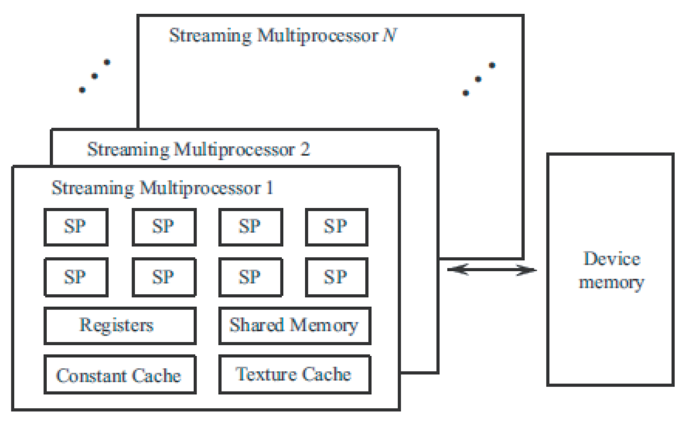
Each GPU consists of a streaming multiprocessor (SM), which contains several scalar processors (SP). The number of SPs depends on GPU type. SM has a number of registers and shared memory used for communication between scalar processors (Figure 3). The instruction set of scalar processors includes arithmetic instructions for real and integer calculations, control instructions (branches and loops), and memory access instructions. RAM access instructions are executed asynchronously. To reduce delays in the GPU execution queue, switching is performed in one clock cycle. The thread manager, which is not programmable, is responsible for switching threads.

The GPU requires algorithm development with a high degree of parallelism on data level. Data array elements (they are data structures or multiple values stored in external memory) are subjected to a single action. One of the GPU’s weakest points is the low bandwidth of the data transmission link between the ALU and external memory. As a result, algorithms that reduce the number of external memory accesses are the most productive, and the ratio of data operations to external memory accesses is at its highest.

3. Memory Access

A significant difference between GPU and CPU is organization of memory and how it is handled. Unlike CPU, which has one type of memory with several levels of caching in the CPU itself, a GPU has a more complex memory structure. Data storage in CPU and GPU memory is illustrated in Figure 4. Shades of gray indicate the speed of access to array elements (the darkest color corresponds to the fastest access to memory).

The construction of CPU memory is one-dimensional (Figure 4a). Due to the caching mechanism, access to adjacent memory elements is fastest. Access to other elements is significantly slower. For example, after reading the array element a[i][j], access to the array elements a[i][j+1] or a[i][j+2] is fast, while access to the array element a[i+1][j] is slow.

In a GPU, memory is organized as two-dimensional array (Figure 4b). Access time is optimal provided that the distance between two array elements is minimal in two-dimensional space. For example, after reading the array element a[i][j], access to the array elements a[i][j+1] or a[i+1][j] is equally fast.

If the padding in bytes between the memory locations of elements $(0,0,0)$ and $(i,j,k)$ for indices $(i,j,k)$ stays constant for both arrays, then the arrays are congruent (congruent padding). If necessary, the arrays are padded with empty elements, which allows for faster memory access [2,10]. This approach is widely used to speed up computations and optimize program code intended for GPUs.

4. Programming Model

The GPU computing model involves the shared use of CPU and GPU resources in a heterogeneous computing model.

The execution of a program using CPU and GPU resources is illustrated in Figure 5. The serial code runs on CPU, and the part of the application that bears the greatest computational load (kernel) runs on the GPU. Scalar processors in a streaming multiprocessor synchronously execute the same instruction, following the SIMD execution model. Multiprocessors are not synchronized, and therefore, the overall execution scheme follows the single instruction multiple threads (SIMP) model.

A kernel and CPU code make up the program code, which is run in several threads using local variables. Kernels are comparatively little processes that use threads for communication and data element processing. A built-in variable in the kernel offers a unique identifier (an integer) to each thread running the kernel. The kernel receives one data element from each input thread, processes the data, and outputs one or more data elements at each stage. A kernel normally processes several data items independently and lacks the internal state.

The execution hierarchy of a program on NVIDIA GPUs is divided into grids of blocks, blocks, and threads (Figure 6), which is related to the structure and organization of memory. Before the kernel is executed, the sizes of the blocks and the grid of the blocks are explicitly specified.

The top level of the hierarchy is the grid. It corresponds to threads executing a given kernel. The grid consists of a 1D or 2D array of blocks. Blocks that form the grid have the same dimension and size. Each block in the grid has a unique address consisting of one or two non-negative integers (the block index in the grid). During execution, the blocks are indivisible and fit into a single SM. The blocks are executed asynchronously. There is no mechanism for synchronizing them. Grouping blocks into grids helps with scaling the program code (blocks are executed in parallel, and blocks are executed sequentially in case of limited resources).

A 1D, 2D, or 3D array of threads makes up each block. One, two or three non-negative numbers that identify thread index within the block make up each thread’s unique address. Each thread in a block has access to shared memory allotted for the block and is synchronized with it. The CUDA programming paradigm designed by NVIDIA allows working with blocks containing from 64 to 512 threads. The number of threads is equal to the number of blocks multiplied by block size. Data are transferred across threads that belong to different blocks using global memory.

An example of a $2\times 3$ grid consisting of six blocks of $(3,1,1)$ threads is shown in Figure 7. Two indices are used to address blocks, and three indices are used to address threads.

Threads within a block are conventionally divided into warps (the minimum amount of data processed by one multiprocessor), which are groups of 32 threads. A streaming multiprocessor processes a warp in 4 cycles. Access to global memory is performed in portions of half a warp (16 threads). The best performance is achieved when transactions involve 32, 64, or 128 bytes. Threads within a warp are physically executed simultaneously. Threads from different warps are at different stages of program execution.

5. Memory Structure

Unlike CPUs, which have one type of memory with several levels of caching in the processor itself, GPUs have a more complex memory organization [2,11]. Part of the memory is located directly in each SM (register, shared memory), and part of the memory is located in DRAM (local, global, constant, texture memory).

NVIDIA graphics processors have several types of memory with different purposes (Figure 8). In this case, CPU updates and requests are only external memory (global, constant, texture).

The comparative characteristics of different types of memory, as well as access rules and allocation levels, are given in

Table 1. Memory types, access rules, and allocation levels.

Memory Type	Access	Allocation Level	Performance
Register	Read/Write	Thread	High
Local	Read/Write	Thread	Low
Shared	Read/Write	Block	High
Global	Read/Write	Grid	Low
Constant	Read	Grid	High
Texture	Read	Grid	High

.

The simplest type of memory is a register file, which is used to temporarily store variables. Registers are located directly in SM and have the highest access speed. Each thread receives a certain number of registers for its exclusive use (registers are distributed between block threads at the compilation stage, which affects the number of blocks executed by the multiprocessor), which are available for both reading and writing. A thread does not have access to the registers of other threads, but its own registers are available to it during kernel execution.

Only one SM has access to a small and relatively slow local memory. Local memory is located in DRAM, and access to it is characterized by high latency. Local memory is used to store local thread variables if there are not enough available registers for this.

Global memory has a high throughput (more than 100 Gb/s for some types of processors) and is used to exchange data between the CPU and GPU. The size of global memory ranges from 256 MB to 1.5 GB depending on the processor type and reaches 4 GB on the NVIDIA Tesla platform.

The simplest solution for organizing data storage and processing on the GPU involves placing them in global memory. Variables in global memory retain their values between kernel calls, which allows using global memory to transfer data between kernels. Working with global memory is not much different from working with regular memory and is intuitive for the developer. Global memory is allocated and freed by calling special functions.

The disadvantage of global memory is its high latency (several hundred cycles), which has a significant impact on the overall speed of calculations. To optimize work with global memory, GPU capabilities are used to combine several requests to global memory into one (coalescing), which allows for almost 16-fold acceleration (accesses to global memory occur via 32, 64, or 128-bit words, and the address at which access occurs is aligned by the word size).

When working with global memory and a large number of threads running on a multiprocessor, the time spent waiting for a warp to access memory is used to execute other warps. Interleaving computations with memory access allows for optimal use of GPU resources [2,11].

To increase the speed of computations, various technologies for accessing shared, constant, and texture memory are used.

Shared memory is located in the multiprocessor itself and is allocated at the block level (each block receives the same amount of shared memory), being available for reading and writing to block threads. A shared memory of 16 KB is equally divided between grid blocks running on the multiprocessor.

Proper use of shared memory plays an important role in writing efficient programs for GPU. Shared memory is used to cache data that are accessed by multiple block threads (instead of storing and retrieving data from the relatively slow global memory). The data caching mechanism, as well as subsequent access to it by the block threads, is organized and programmed by the developer. Given the limited size of the shared memory allocated to each block, creating an effective mechanism for accessing shared memory is non-trivial and complicates the program code. Shared memory is also used to pass parameters when starting the kernel for execution. Constant memory is used to pass a large volume of input parameters passed to the kernel in the construction of its call.

Shared memory usually requires the use of synchronization functions after data copying and modification operations. To increase throughput, the shared memory is divided into 16 modules, each of which performs one read or write of a 32-bit word [2] (access to the modules occurs independently). When 16 threads access 32-bit words, the number of which is half of the warp and which are located in different modules, the result is obtained without additional delays. If there are several requests coming to the same module, the requests are processed sequentially, one after another (a module conflict occurs). In the case where threads access the same element, there is no module conflict [11]. To avoid conflicts over memory modules, a certain number of empty elements are added to the original data (this technique allows for word boundary alignment for access to global memory).

A constant memory of 64 KB is cached by 8 KB for each multiprocessor, which makes repeated reading of data quite fast (much higher than the speed of access to global memory). This memory is used to place a small amount of frequently used unchangeable data, which are accessible to threads. Memory allocation occurs directly in the program code. If the necessary data are not in the cache, there is a delay of several hundred cycles. Using constant memory is no different from using global memory on CPU.

Texture memory implements fixed functionality for accessing certain areas of memory, accessible only for reading. The emergence of texture memory is associated with the specifics of graphics applications [2] (shading triangles using a two-dimensional image called a texture). Texture is a simple and convenient interface for read-only access to 1D, 2D, and 3D data. Using texture memory seems appropriate in the case when it is not possible to ensure the fulfillment of conditions for combining requests. An additional advantage of texture memory is the texture cache (cached by 8 KB for each multiprocessor).

Constant and texture memory are available to mesh threads, but only for reading, and writing to them is performed by the CPU by calling special functions. From the developer’s point of view, using constant and texture memory is not labor-intensive and slightly complicates the program code.

With proper use of shared memory, the additional speedup of the calculation is from 18 to 25% (depending on the technology and optimization methods), and when using constant and texture memory, the speedup of the calculation reaches 35–40% [12].

6. Data Distribution

When using systems with parallel data processing and parallelization of computational algorithms using MPI or OpenMP technologies, the simplest way is to decompose $n_x\times n_y\times n_z$ nodes in one direction into N blocks, each of which has size $(n_x/N+m)\times n_y\times n_z$, where m is the number of ghost cells used for data exchange between processors (in particular, $m=3$ for 5th-order scheme and $m=5$ for 9th-order scheme). An example of domain decomposition is presented in Figure 9.

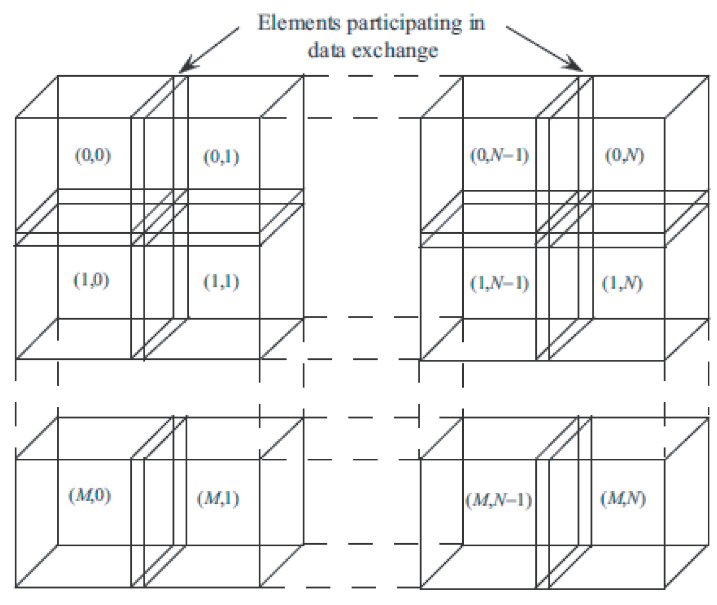
The input data array, such as array fluid quantities at mesh nodes, is split up into several blocks to carry out parallel computations on the GPU (Figure 10). A grid of size $M\times N$ is formed by blocks. It is assumed that each block has 32 threads, which is a multiple of the warp size. An intersection between neighboring blocks permits the exchange of boundary data between blocks, ensuring accuracy.

Typically, shared memory is used for data exchange between blocks. However, when one thread processes data in a single mesh cell, shared memory need not be used.

7. Single and Double Precision

The highest performance is achieved with single-precision calculations. When using double-precision, performance is theoretically reduced by an order of magnitude (compared to peak performance declared by manufacturer) and approximately twice as much in practice [12]. The reduction in the performance of calculations on the GPU is significantly greater than on the CPU, which affects calculations that require increased precision.

Calculations performed in [10] show that double-precision calculations are approximately 46–66% (depending on the mesh size) slower than single-precision calculations. The peak performance of double-precision computations (78 GFlops for NVIDIA GT200) is 12 times slower than the performance of single-precision computations (936 GFlops for NVIDIA GT200). Finite-difference calculations performed in [13] show that double-precision computations are approximately 2–3 times slower than single-precision computations.

The potential of mixed-precision computations is discussed in [14,15]. Single precision is used to compute the left-hand side of a discrete equation, which is related to time discretization, and double precision is applied to compute the right-hand side, which is residual due to discretization of inviscid and viscous fluxes [15] ( the sequential part of code running on the CPU uses double-precision computations). This approach allows for gains in computational performance without loss of accuracy.

8. Problem Solving

Solving a problem using GPU involves the following sequence of steps (the pattern is typical but not mandatory).

1. Creating a program for the CPU and solving the problem using any known programming languages (e.g., C/C++, Fortran).

2. Selecting program sections (kernels) that perform intensive calculations. This is performed using a profiler, understanding the program structure and any other considerations.

3. Determining whether specific kernels need to be transferred to the GPU. Some kernels (e.g. matrix multiplication and some other linear algebra operations) are implemented on GPU and are available as libraries of standard functions.

4. Refactoring the original program. Each kernel that seems justified for transfer to the GPU is allocated as a separate function. The function itself is reorganized in such a way as to eliminate side effects, as well as arrays shared with other parts of the program. To avoid unnecessary transfers not only the kernel is transferred to GPU but also adjacent code, the transfer of which without the kernel is not justified.

5. Selecting a programming technology (NVIDIA uses CUDA technology, while AMD uses CTM technology).

6. Implementing the kernel using the selected programming technology (the most difficult issue is related to using different types of memory).

7. Further optimization of the kernel performance, related to changing the partitioning of the source data into blocks and using different types of memory to speed up calculations.

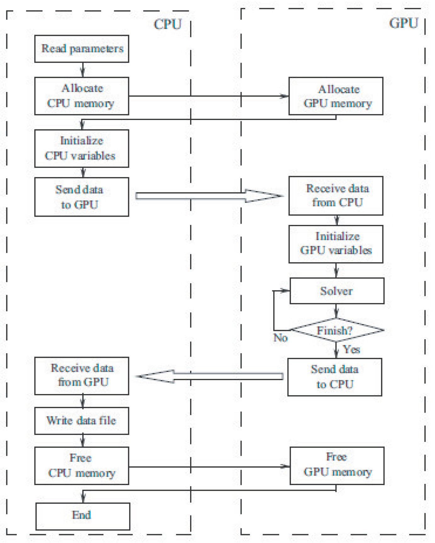
The diagram of solving the problem on the GPU is explained in Figure 11 (step 6). The preparation of input data (reading from the hard disk, forming and initializing arrays, sorting) is performed on the CPU. Data arrays are copied to the GPU (the bandwidth of the bus through which data are copied is about 5 Gb/s). Intensive computations are performed on GPU. A given sequence of actions is performed on GPU over the data arrays. Each thread processes one mesh node. The resulting arrays are copied from GPU to CPU, after which data are processed and visualized and saved to the hard drive.

The scheme depicted in Figure 12 is applied to solve the governing equation in CFD with the finite volume method. The CPU prepares initial data, which include mesh node coordinates, boundary conditions, and data structure for storing the unstructured mesh topology. The quantities are initialized, and data are copied to the GPU global memory. The GPU solves the system of algebraic equations using the iterative method, computes inviscid and viscous fluxes, and advances solution in time. Different kernels are used on the GPU to carry out calculations at the internal and boundary nodes (per different rules). Convergence is examined on the CPU. When the norm of the residual is copied to CPU memory, synchronization between the CPU and GPU is required to verify the convergence condition. The quantities are moved from the GPU to CPU memory once the convergence condition is satisfied.

The maximum sound speed for mesh cells at each time step is determined in order to verify Courant–Friedrichs–Lewy condition (CFL stability condition). The reduction summation method and its modifications are employed for this purpose [2].

The kernel implementation depends on the chosen programming technology and is the most complex step in the software implementation of the code for the GPU.

9. Programming Technology

Practical problems on GPUs are solved with various programming technologies, the use of which usually requires knowledge of the details of GPU architecture. Many programs written for GPUs are low-level, difficult to maintain, and non-portable. Programming strategies and trends in development of programming and debugging tools for GPUs are discussed in [16].

Graphics programming technologies include the 3D graphics programming interface and the shader language. The shader language is a C-like programming language that eliminates pointers and adds GPU-specific data types and operations. Graphics programming tools support the compilation and execution of graphics programs and include libraries of graphics functions related to pixel and fragment processing.

Low-level programming technologies emerged as GPU manufacturers recognized the commercial importance of their use for high-performance computing. Low-level programming tools consist of an intermediate assembler intended for compiler and programming language developers and a C-like language intended for writing programs that use GPU resources.

For GPUs manufactured by NVIDIA, the main programming tool is Compute Unified Device Architecture (CUDA) technology, which uses a dialect of C language (C for CUDA) as a programming language, extended by some additional tools (for example, special keywords for describing kernels, constructions for starting calculations, and others). There is also Java for CUDA (JCUDA) technology, intended for use in conjunction with Java language. For AMD, close to metal (CTM) programming technology is used.

One of the high-level programming languages for GPUs is the Open Computing Language (OpenCL), developed by Apple for streaming programming. The OpenCL language, like Open Graphics Library (OpenGL), is a library that can be used from any programming language.

Comparison of the performance of different technologies (CUDA, JCUDA, OpenCL) and evaluation of the efficiency of program optimization methods on GPU are considered in [12]. To ensure data synchronization when performing calculations on several video cards distributed in the network, inter-network interaction technologies (MPI, OpenMP) are used. Comparison of the obtained results shows that the programming technologies differ slightly from each other in the achieved code performance, as well as in ease of use. The difference in performance between CUDA and JCUDA implementations is insignificant. The performance of calculations on the GPU is more than 38 times higher than performance of calculations on the CPU of a supercomputer and almost 9 times higher than the performance of calculations on a four-core CPU using OpenMP technology.

When using optimization technology, the code for the GPU becomes more complex, and its size is approximately 3–4 times larger than the code in C++ language.

10. CUDA Technology

To support non-graphical applications on NVIDIA GPUs, the unified computing architecture CUDA is used. It is based on an extension of C language and allows access to the GPU instruction set for managing its memory [2]. The GPU is considered a computing device capable of supporting the parallel execution of a large number of threads or streaming programs (GPU is a coprocessor of the host computer CPU). Optimized data exchange between the CPU and GPU is implemented. Both 32-bit and 64-bit operating systems are supported. Type specifiers, built-in variables and types, kernel startup directives, and other functions are added to the programming language.

A number of functions are used only by the CPU (CUDA host API). These functions are responsible for managing the GPU, working with context, memory, modules, and also managing code execution and working with textures. The functions are divided into synchronous and asynchronous. Synchronous functions are blocking, while other functions (copy, kernel startup, memory initialization) allow asynchronous calls.

The functions provided to the developer of the program code are available in the form of low-level API (CUDA driver API) and high-level API (CUDA runtime API). Although low-level API provides more extensive programming capabilities, its use leads to a large amount of code, as well as the need for explicit settings and initialization in the absence of emulation mode (compilation, launch, and debugging of code on CUDA when using CPU).

Thread blocks are separated into grids, and threads are separated into thread blocks. Threads inside a block are conventionally divided into warps, each of which is a group of 32 threads. The number of blocks times block size equals the number of threads. The built-in variable threadIdx is a structure of three fields that correspond to three Cartesian coordinates. It provides a unique identifier (integer) for each thread running the kernel inside the block. A block in the grid with two-dimensional addressing is identified by the built-in variable blockIdx. A built-in variable called blockDim and another called gridDim provide the block and grid sizes, respectively, and are accessible to every thread.

Global memory is allocated by calling the function cudaMalloc on CPU or by declaring a variable in the kernel body using the keyword __device__.

The kernel is declared using the keyword __global__ before the function definition. The kernel is called using the kernelName<<<dimGrid,dimBlock>>> (chevron syntax) construct. The variables dimGrid and dimBlock, of type dim3, specify the grid dimension and size in blocks and the block dimension and size in threads.

A simplified implementation of the code that calculates flows through the edges of a control volume (2D problem) is considered. For this purpose, mesh cells are iterated and the contribution of each face of control volume is taken into account. The code is given with some abbreviations that are not essential for understanding the implementation features.

     // CPU

     void flux(){

        for (i=1; i<nx-1; i++)

          for (j=1; j<ny-1; j++)

            v[i][j]=a*u[i+1][j]+b*u[i-1][j]+c*u[i][j+1]+d*u[i][j-1]+...

     }

     // GPU

     __global__ void flux(){

        int i=blockIdx.x*blockDim.x+threadIdx.x;

        int j=blockIdx.y*blockDim.y+threadIdx.y;

        int k=nx*j+i;

        if ((0<i) && (i<nx-1) && (0<j) && (j<ny-1)){

          int ke=nx*j+(i+1);

          int kw=nx*j+(i-1);

          int kn=nx*(j+1)+i;

          int ks=nx*(j-1)+i;

          v[k]=a*u[ke]+b*u[kw]+c*u[kn]+d*u[ks]+...

        }

     }

Here, v is the array that stores the fluxes, and u is the array that stores the velocity. Coefficients a, b, c, and d are determined by numerical scheme. In the CPU program, velocity and fluxes are stored in a 2D array, while in the GPU code, they are stored in a 1D array. The mesh sizes are nx and ny in x and y directions.

CPU code is implemented as two nested loops that iterate over mesh nodes in x and y directions. When implementing code for GPU, geographic notation is used to denote the nodes, and indices of the corresponding array elements are found with thread identifier, block identifier, and thread block size.

A thread block is executed on SM, and threads within the block exchange data via shared memory. To avoid problems when working with shared memory, a barrier mechanism for synchronizing block threads is used. To implement synchronization, a call to the built-in function __syncthreads is used, which blocks the calling threads of the block until block threads enter this function (waiting for the completion of operations previously called from this CPU thread).

CUDA technology provides the programmer with a number of libraries (CUFFT, Fast Fourier Transform library; CUBLAS, linear algebra library; CUSPARSE, library of functions for working with sparse matrices; CURAND, library for generating random numbers, and others). The set of functions of the BLAS library is implemented in CUDA SDK, which is used together with existing programs that work with BLAS (among such programs, for example, is the MATLAB package).

11. Programming Implementation

The increase in CPU performance is associated with an increase in clock frequency and the size of high-speed cache memory. Programming for resource-intensive scientific computations implemented on the CPU implies structuring data and the order of instructions to efficiently use levels of cache memory. In contrast to the CPU, the GPU is an example of SM, which uses data parallelism to increase the speed of computation and reduce dependence on memory access latencies. In the concept of stream computing, data are represented as streams of independent elements, and independent processing stages (sets of operations) are represented as kernels. Kernels are in the form of a function for transforming elements of input streams into elements of output streams, which allows the kernel to be applied to many elements of the input stream in parallel.

11.1. Data Types

The increase in the speed of computations on the GPU is achieved through the use of vector data types (type float4), defined in CUDA [15].

A single transaction is used in the GPU to copy 128-bit words from the device memory to registers. It is quicker to load a float4 variable into registers from the device memory than it is to load four float variables using four transactions.

This approach is relatively easy to apply in calculations of 2D laminar compressible fluid flows, when the flow state is described by four variables (single-precision calculations). For calculations of 3D laminar flows or 2D turbulent flows (single- or double-precision calculations), when the number of fluid quantity increases to five, aligned user-defined data types are used, which guarantees a minimum number of transactions when accessing memory. For example, using this approach in double-precision calculations allows access to five double-precision variables using three 128-bit transactions instead of five.

The location of block vectors in memory has an impact on GPU computation performance. Each control volume in the finite volume method implementation is equivalent to five physical variables (density, three velocity components, pressure). In CPU calculations, $n_e$ blocks of five fluid quantities are written to expand the data into a linear array. Using the ordinal number j in control volume i to address the desired function has the form u[5*i+j]. Expanding the data into five blocks of $n_e$ values, or addressing u[i+j*n_e], is a more effective addressing technique for GPUs. The code performance is improved by this arrangement of vectors in memory, which is consistent with the coalescing model.

11.2. Memory Usage

To optimize code performance, the amount of data transferred between the CPU and GPU is reduced. For this purpose, shared memory and texture memory are used (both memories are cached). Shared memory is managed at the software level, which complicates the logical construction of the program code. The texture memory cache is managed at the hardware level. Using texture memory improves the computational performance by approximately 1.5 times [10].

Reducing the quantity of global memory accesses in every thread optimizes performance. The discrete equation left and right sides are calculated at each mesh node by counting the faces connected to the node and adding up the contributions of fluxes through those faces. By making extensive use of shared memory and updating variables stored in global memory after calculations are finished, it is possible to reduce the number of global memory accesses.

The information needed at the evolution step is computed prior to the time step beginning and saved in texture memory when different numerical schemes are implemented. Global memory is where the outcomes from the time step are kept. The parameters are determined in the dummy cells of each block rather than sharing information between neighboring blocks that correspond to dummy cells.

Using texture memory allows for gaining performance. Texture memory size is limited. Texture memory usually stores arrays of data that are accessed arbitrarily (unstructured) in the program but which are often involved in the iteration process, and their values are updated only once [15]. Such data include primitive variables and their gradients, which are involved in calculating inviscid and viscous fluxes. Primitive variables are found from known values of conservative variables and are stored in texture memory at the beginning of the integration step. The kernel that calculates inviscid and viscous fluxes extracts fluid quantities and their gradients from texture memory, reducing time per iteration.

One of the problems in implementing many iterative methods on the GPU is the large number of synchronization points for calculations, which leads to an increase in read/write operations for data in the slow global memory of device and a reduction in the number of calculations in fast memory. The performance of the iterative method on GPUs can be improved by grouping computations to reduce access to slow memory and performing asynchronous operations of copying device memory.

11.3. Coalesced Query

When using unstructured meshes, it is difficult to coalesce multiple global memory requests into one (coalesced memory access) due to the unordered numbering of mesh nodes, faces, and cells (the kernel that calculates the flows enumerates mesh faces associated with the node).

There are significant differences in the implementation of the finite volume method on unstructured mesh if the control volume coincides with the mesh cell (cell-centered scheme) [17], and control volume is constructed near the mesh node (vertex-centered scheme) [15]. When using control volumes that coincide with mesh cells, the kernel enumerates a fixed number of faces and a fixed number of adjacent nodes. When using a scheme in which control volumes are built around mesh nodes, the number of faces associated with a given node is not fixed, resulting in additional global memory accesses.

To optimize the work with global memory, a renumbering scheme is used, which ensures that the faces participating in parallel computation of flows are located adjacently in the global memory. This approach increases the computational performance by approximately 70% in the 3D case [15].

11.4. Thread Intersection

The implementation of the finite volume method follows a set of similar tasks requiring processing for computing fluxes through the faces of control volumes. To calculate the flux through an internal face, the flow quantities in the control volumes to which this face belongs and its geometric parameters (area, normal) are used. To calculate the flux through a boundary face, in addition to face geometric parameters, fluid quantities in the control volume adjacent to the boundary of the region are used. Fluid variables are considered constant within the time integration step, so the tasks for computing flows are independent in input data.

One of the problems of implementing computational algorithms within the shared memory model is the data intersection between parallel threads [3,15]. The presence of critical sections and atomic operations that limit the simultaneous access of threads to data leads to a significant decrease in performance.

Thread intersection occurs, for example, when summing fluxes [3,15]. The flux through the common edge of two control volumes i and j is calculated using one or another numerical scheme. The fluxes are summed over the control volumes into the corresponding arrays, which are used to find fluid variables at a new time layer. When parallelizing fluxes through edges $(i,j)$ and $(i,k)$, there is the possibility of an error occurring when fluxes for control volume i are summed simultaneously by two different threads. When developing algorithms for GPUs, the thread crossing problem is solved by computing fluxes with data replication and per-cycle flux computation [3].

In the case of flux calculation with data replication, to avoid conflicts in memory access at the flux calculation stage, an additional array is created to store fluxes through faces of control volumes. This approach increases the consumption of RAM, since two sets of five quantities (density, three velocity components, pressure) are recorded for each edge. After calculating the fluxes through the edges, the flows are summed to obtain the final values in the control volumes. This requires storing in memory a dual graph of control volume connections (the graph vertices are the control volumes, and edges are the connections of control volumes through their common edges), which contains $2n_c+n_e+1$ integer values, where $n_c$ is the number of mesh cells, and $n_e$ is the number of internal edges of the control volumes.

In the per-cycle computation of fluxes, an edge coloring scheme is applied to the dual mesh graph. From the set of graph edges, a subset of edges is selected in which each node occurs no more than once. The processing of such a subset of edges by threads running on a GPU occurs in parallel and eliminates the possibility of thread conflicts in modifying the same memory cells. The procedure for calculating fluxes is divided into cycles. At each of these cycles, one of the selected subsets of cell edges is processed. The number of cycles for calculating fluxes exceeds the maximum number of faces of the control volume (e.g., for a mesh with hexahedron-shaped cells, the number of cycles exceeds six), and the number of faces simultaneously processed at each cycle does not exceed $n_e/2$. The need to repeatedly launch the procedure for calculating fluxes for each cycle and a decrease in the number of simultaneously processed faces are negative features of the approach. However, there is no need to allocate additional amounts of RAM and unnecessary summation of fluxes calculated by faces in cells.

A comparison conducted in [3] shows that the replication-based flow computation method is 17% faster than the cycle-based flow computation method.

11.5. Conditional Operator

There are some peculiarities associated with the execution of some instructions with branches. The problem with the execution of the conditional jump operator (if/else operator) is that computing devices of the multiprocessor execute the same instruction, and the conditional jump instruction directs different threads of the same group (from the same warp) to different code chains.

The execution of the conditional jump instruction is carried out by dividing group of threads into two subgroups. For one subgroup, the conditional jump is not performed, and for the other, it is performed (both subgroups of threads are executed one after the other, which leads to an increase in total calculation time).

In this case, the tool for implementing the conditional jump operator is predicates, which are single-bit registers that store the results of comparisons and allow references from the instruction. The presence of a reference in the instruction code from a logical point of view means its conditional execution (the operation is performed if the predicate value is true). Each computing device of the multiprocessor has an individual set of predicates, so the decision to execute an instruction referring to a predicate is made for each thread separately (for some threads the instruction is executed, but for others, it is not).

11.6. Numerical Scheme

The implementation of the 2nd order smoothing scheme on a three-dimensional structured mesh (the control volumes are cubes) is considered

$$\begin{array}{c}\hfill b_{i,j,k}=(1-s)a_{i,j,k}+{\displaystyle \frac{s}{6}}\left(a_{i-1,j,k}+a_{i+1,j,k}+a_{i,j-1,k}+a_{i,j+1,k}+a_{i,j,k-1}+a_{i,j,k+1}\right).\end{array}$$

The s factor controls the smoothing.

It is assumed that the computational domain is one block of size $(n_x-2)\times (n_y-2)\times (n_z-2)$. In memory, the grid block is represented as a 3D array of size $n_x\times n_y\times n_z$. For the 3rd order difference scheme, two nodes are added in each coordinate direction (one node on each side of the block to store the boundary values).

The code for the CPU is implemented based on nested loops and the enumeration of mesh nodes (elements of the array in which the values of the mesh function are stored).

     // CPU

     float a(nx,ny,nz),b(nx,ny,nz),s;

     smooth(a,b,s);

     ...

     // finite difference scheme

     void smooth(float *a,float *b,float s){

       for (k=2; k<=nz-1; k++)

         for (j=2; j<=ny-1; j++)

           for (i=2; i<=nx-1; i++)

             b[i][j][k]=(1.0-s)*a[i+1][j][k]+

                        s*(a[i-1][j][k]+a[i+1][j][k]+a[i][j-1][k]+

                           a[i][j+1][k]+a[i][j][k-1]+a[i][j][k+1])/6.0;

     }

Implementing the code when using GPU involves allocating memory, calling a function, and the body of the kernel function in C (CPU code) and CUDA (GPU instructions). The GPU code is several times longer than the CPU code.

      1 // macro for 3D to 1D index translation

      2 #define I3D(ni,nj,i,j,k) ((i)+(ni)*(j)+(ni)*(nj)*(k))

      3

      4 float *a_cpu,*a_gpu,*b_gpu,s;

      5

      6 // allocate memory on host (CPU)

      7 nbyte=sizeof(float)*ni*nj*nk;

      8 a_h=malloc(nbyte);

      9 // allocate memory on device (GPU)

     10 cudaMalloc(&a_d,nbyte);

     11 cudaMalloc(&b_d,nbyte);

     12

     13 // transfer memory from host to device

     14 cudaMemcpy(a_d,a_h,nbyte,cudaMemcpyHostToDevice);

     15

     16 // GPU kernel parameters

     17 num_threadblocks=dim3(1,1,1); // single thread block

     18 num_threads=dim3(ni,nk,1);    // plane of threads

     19 // call GPU kernel

     20 smooth_kernel<<<num_threadblocks,num_threads>>>(a_d,b_d,s);

     21

     22 // kernel

     23 __global__ void smooth_kernel(float *a_data,float *b_data,float s){

     24   int i,j,jm1,jp1,k,j_plane;

     25   // shared memory for three planes

     26   __shared__ float a[ni][3][nk];

     27

     28   // current thread index

     29   i=(int)threadIdx.x;

     30   k=(int)threadIdx.y;

     31

     32   // fetch the first planes into shared memory

     33   a[i][0][k]=a_d[I3D(ni,nj,i,0,k)];

     34   a[i][1][k]=a_d[I3D(ni,nj,i,1,k)];

     35

     36   // set initial jm1,j,jp1

     37   jm1=0; j=1; jp1=2;

     38

     39   // iterate upwards in j direction

     40   for (j_plane=1; j_plane<nj-1; j_plane++){

     41

     42     // read next plane into jp1 slot

     43     a[i][jp1][k]=a_d[I3D(ni,nj,i,j_plane+1,k)];

     44     // make sure reads into shared memory are done

     45     __syncthreads();

     46

     47     // ghost-zone threads do not compute

     48     if (i>0 && i<ni-1 && k>0 && k<nk-1){

     49       // apply stencil and write out result

     50       i000=I3D(ni,nj,i,j,k);

     51       b_d[i000]=(1.0f-s)*a[i][j][k]+

     52                 s*(a[i-1][j][k]+a[i+1][j][k]+a[i][jm1][k]+

     53                    a[i][jp1][k]+a[i][j][k-1]+a[i][j][k+1])/6.0f;

     54     }

     55     // cycle j indices

     56     tmp=jm1; jm1=j; j=jp1; jp1=tmp;

     57   }

     58 }

The GPU code allocates memory for both the variables stored in CPU memory (lines 7 and 8) and the variables stored in GPU memory (lines 10 and 11). Line 14 shows the copying of variables from CPU memory to GPU memory. It is necessary to call special functions that are prefixed with cuda for any operations that access GPU memory outside of the kernel. Many threads execute the kernel concurrently, so the number and arrangement of threads must be specified. Line 17 assumes that there is a single block of threads, which form a plane (line 18), for simplicity’s sake. The necessary number of blocks and threads is specified when calling the kernel (line 20). The kernel function is called by the CPU and run on the GPU, as indicated by the keyword __global__ (line 23). The __shared__ keyword (line 26) declares the array containing the calculated values, indicating that it is kept in shared memory. The coordinates of i and k in the block plane (lines 29 and 30) are determined by each thread using the built-in variable threadIdx. The offset with respect to $j-1$, j, and $j+1$ planes is stored in shared memory using the variables jm1 and jp1 (line 37). These indices are swapped out for new ones at the conclusion of each iteration (line 57). Lines 33, 34, and 43 copy data from the global-memory-stored a_d array to the shared-memory-stored a array. To make sure that threads have completed loading data before running the subsequent code (synchronization), the __syncthreads function (line 45) is called. The outer threads do not take part in the computations carried out by the inner threads; instead, they load data from dummy cells (line 48).

12. Solution of Laplace Equation

The solution of the Laplace equation $\Delta u=0$ in the 2D square domain with unit side $\Omega =(0,1)\times (0,1)$ is considered. On the left, right, and lower boundaries, it is assumed that $u=0$, and on the upper boundary, it is assumed that $u=1$.

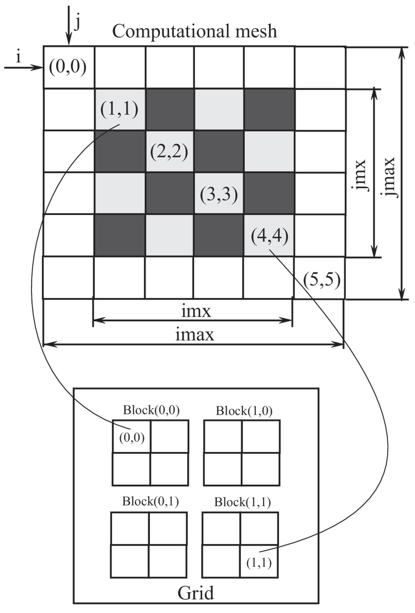
A uniform rectangular mesh with a cross node template is subjected to the finite difference method in order to discretize the Laplace equation. The Gauss–Seidel method or successive over-relaxation method with red/black parallelization are used to solve system of difference equations. Figure 13 shows how the computational domain is mapped onto GPU memory structure. A mesh comprising imax×jmax nodes is used for the computations. The code does not process a number of nodes, which are used to set boundary conditions (the corresponding cells are highlighted in white). imx×jmx nodes are processed by the code.

An explicit difference scheme for the Laplace equation on a uniform mesh using geographic notation for mesh nodes (n is north, s is south, e is east, w is west) is

$$\begin{array}{c}\hfill u_p^{n+1}={\displaystyle \frac{1}{a_p}}\left(a_n{u}_n^n+a_s{u}_s^n+a_e{u}_e^n+a_w{u}_w^n\right),\end{array}$$

where $a_p=a_n+a_s+a_e+a_w$. The solution at iteration $n+1$ is

$$\begin{array}{c}\hfill u_p^{n+1}:=\omega u_p^{n+1}+(1-\omega )u_p^n,\end{array}$$

where $\omega$ is the relaxation parameter. Nodes n, s, e, and w surrounding node p have the same color.

Allocating dynamic memory; setting initial and boundary conditions; calculating the coefficients $a_n$, $a_s$, $a_e$, and $a_w$; allocating memory on GPU; copying variables from CPU to GPU; establishing block and grid sizes; calling kernel for red nodes and calling kernel for black nodes; and copying results from GPU to CPU are steps that make up the GPU code.

In order to implement the code that is called on CPU, the block size and grid size must be specified. Additionally, the kernels that are launched on the GPU to process the black and red nodes must be called.

    // configuration definition

    dim3 dimBlock(BLOCK_SIZE,BLOCK_SIZE);

    dim3 dimGrid(imx/BLOCK_SIZE,jmx/BLOCK_SIZE);

    // iteration loop

    for (iter=1; iter<=itmax; iter++){

      // run kernel to update red nodes

      red_kernel<<<dimGrid,dimBlock>>>(u_old_d,an_d,as_d,ae_d,aw_d,ap_d,imx,jmx);

      // run kernel to update black nodes

      black_kernel<<<dimGrid,dimBlock>>>(u_old_d,an_d,as_d,ae_d,aw_d,ap_d,imx,jmx);

    }

The code running on the GPU is implemented using processing nodes that are the same color (the kernels for black and red nodes are implemented using the same scheme).

    // relations between threads and mesh cells

    // global thread indices (tx,ty)

    int tx=blockIdx.x*BLOCK_SIZE+threadIdx.x;

    int ty=blockIdx.y*BLOCK_SIZE+threadIdx.y;

    // convert thread indices to mesh indices

    row=(ty+1);

    col=(tx+1);

    // Gauss-Seidel method (SOR)

    if ((row+col)%2==0){

      // red cell

      float omega=1.85,sum;

      k=row*imax+col;

      // perform SOR on red nodes

      sum=aw_d[k]*u_old_d[row*imax+(col-1)]+ae_d[k]*u_old_d[row*imax+(col+1)]+

          as_d[k]*u_old_d[(row+1)*imax+col]+an_d[k]*u_old_d[(row-1)*imax+col];

      u_old_d[k]=u_old_d[k]*(1.0-omega)+omega*(sum/ap_d[k]);

    }

The solution is saved on the GPU as $m\times n$ matrix, where each matrix contains the fluid quantities in internal and boundary nodes. Parallel computations are carried out in $n/2$ blocks, each of which has $m-2$ threads. Because each thread in the block writes a single value to the shared memory, thread access to the necessary data is accelerated, and the likelihood of two concurrent accesses to the same dynamic memory element is decreased.

Laplace equations solving on GPU is about 22 times faster than on the CPU (only global memory is used in calculations).

13. Projection Method

The projection method and finite volume method on uniform mesh with a staggered arrangement of nodes are used to solve Navier–Stokes equations describing unsteady flow of viscous incompressible fluid [18].

The following formulas describe the unsteady flow of viscous incompressible fluid

$$\begin{array}{cc}\hfill & \nabla ·v=0;\hfill \end{array}$$

(1)

$$\begin{array}{cc}\hfill & {\displaystyle \frac{\partial v}{\partial t}}+\left(v·\nabla \right)v=-{\displaystyle \frac{1}{\rho }}\nabla p+\nu \Delta v+f.\hfill \end{array}$$

(2)

Here, f is the external force per unit volume. For simplicity of notation, the dependence of the transport coefficients on spatial coordinates is not taken into account. The buoyancy effects due to the temperature gradient are considered using the Boussinesq approximation. The representation of the external force per unit volume is

$$\begin{array}{c}\hfill f=\left[1-\beta \left(T-T_0\right)\right]g,\end{array}$$

where $\beta$ is the coefficient of volume expansion, and $T_0$ is the reference temperature.

The velocity v and pressure p are presumed to be known at time $t_n$. Fluid quantities at time $t_{n+1}$ are then calculated using the projection method [19,20].

It is assumed that only convection and diffusion are responsible for the momentum transfer at stage 1

$$\begin{array}{cc}\hfill & {\displaystyle \frac{\tilde{v}-v^n}{\Delta t}}=-\left(v^n·\nabla \right)v^n+\nu \Delta v^n+f^n.\hfill \end{array}$$

(3)

The intermediate velocity $\tilde{v}$ has physical significance even though it does not satisfy the continuity equation. It is possible to derive that $\mathrm{rot}\tilde{v}=\mathrm{rot}{v}^{n+1}={\omega }^{n+1}$ by applying the rotor operator to Equations (2) and (3), accounting for the fact that $\mathrm{rot}\nabla p=0$. The vortex properties are maintained by the intermediate velocity field at the interior points.

At stage 2, the solenoidality of velocity vector $v^{n+1}$ is taken into consideration when calculating pressure from discovered intermediate velocity $\tilde{v}$

$$\begin{array}{cc}\hfill & \Delta p^{n+1}={\displaystyle \frac{1}{\Delta t}}\nabla ·\tilde{v}.\hfill \end{array}$$

(4)

At each time step, Poisson Equation (4) is solved using either direct or iterative methods.

At stage 3, it is believed that the pressure gradient alone is responsible for the momentum transfer; neither convection nor diffusion are present.

$$\begin{array}{cc}\hfill & {\displaystyle \frac{v^{n+1}-\tilde{v}}{\Delta t}}=-\nabla p^{n+1}.\hfill \end{array}$$

(5)

Taking into consideration the continuity equation $\nabla v^{n+1}=0$, Poisson Equation (4) is obtained by taking the divergence of both sides of Equation (5).

Convective and diffusion fluxes are discretized using countercurrent and centered second-order differences, while time is discretized using the Adams–Bashworth scheme. The Gauss–Seidel method employing red/black parallelization and the bi-conjugate gradient with stabilization (BiCGStab) method solves the Poisson equation for pressure.

A set of $n_z$ matrices, each of size $n_x\times n_y$, is used to represent a mesh of size $n_x\times n_y\times n_z$ on the GPU (Figure 14). The code does not process certain nodes. They are used to set boundary conditions. When using global memory, this mesh mapping from the CPU to GPU is practical.

Two nested loops make up parallel code on a single GPU that implements the projection method. The inner loop integrates the Poisson equation using the Jacobi iteration method (or another iteration method), while the outer loop advances the solution in time. Fluid quantities at time layer n are only variables that affect the solution at layer $n+1$ when employing the Euler scheme. Six matrices (three for each time layer) are used to store the velocity at the mesh nodes on two adjacent time layers. At the conclusion of each time step, their values are swapped. Two matrices are used to store the pressure on two adjacent time layers, and at the conclusion of each iteration, their values are swapped.

     //copy data from CPU to GPU

     ...

     // time-stepping loop controlled on CPU

     // for each time step

     for (t=0; t<ntstep; t++){

       // call kernel to compute momentum (ut,vt,wt)

       momentum<<grid,block>>(u,v,w,uold,vold,wold)

       // call kernel to compute boundary conditions

       momentum_bc<<grid,block>>(u,v,w)

       // call kernel to compute divergence (div)

       divergence<<grid,block>>(u,v,w,div)

       // for each Jacobi solver iteration

       for (j=0; j<njacobi; j++){

         // call kernel to compute pressure

         pressure<<grid,block>>(u,v,w,p,pold,div)

         // rotate matrices

         ptemp=pold; pold=p; p=ptemp;

         // call kernel to compute boundary conditions

         pressure_bc<<grid,block>>(p)

       }

       // call kernel to correct velocity (ut, vt, wt)

       correction<<grid,block>>(u,v,w,p)

       // call kernel to compute boundary conditions

       momentum_bc<<grid,block>>(u,v,w)

       // rotate matrices

       utemp=uold; uold=u; u=utemp;

       vtemp=vold; vold=v; v=vtemp;

       wtemp=wold; wold=w; w=wtemp;

     }

     // copy data from GPU to CPU

     ...

The primary steps of the projection method are implemented by the six cores of the parallel code running on multiple GPUs. Before going on to the next layer in time, different cores are running to guarantee global synchronization between blocks.

     // for each time step

     for (t=0; t<steps; t++){

       // copy velocity ghost cells from host to GPU

       ...

       // call kernel to compute momentum

       momentum<<<grid,block>>>(u,v,w,uold,vold,wold,gpuCount,*device);

       // apply boundary conditions

       momentum_bc<<<grid,block>>>(u,v,w,gpuCount,*device);

       // copy velocity border cells from GPU to host memory

       ...

       // synchronize with other threads before reading updated ghost cells

       pthread_barrier_wait(&barrier);

       // copy velocity ghost cells from host to GPU

       ...

       // call kernel to compute divergence

       divergence<<<grid,block>>>(u,v,w,div,gpuCount,*device);

       // for each Jacobi solver iteration

       for(m=0; m<njacobi; m++){

         // compute pressure

         pressure<<<grid,block>>>(div,pold,p,gpuCount,*device);

         // rotate matrices

         ptemp=pold; pold=p; p=ptemp;

         pressure_bc<<<gridDims,blockDims>>>(d_p,s_gpuCount,*device);

         // copy pressure border cells from GPU to host memory

         ...

         // synchronize with other threads before reading updated ghost cells

         pthread_barrier_wait(&barrier);

         // copy pressure ghost cells from host to GPU

         ...

       }

       // velocity correction

       correction<<<grid,block>>>(u,v,w,p,gpuCount,*device);

       momentum_bc<<<grid,block>>>(u,v,w,gpuCount,*device);

       // copy velocity border cells from GPU to host memory

       ...

       // synchronize with other threads before reading updated ghost cells

       pthread_barrier_wait(&barrier);

       // rotate matrices

       utemp=uold; uold=u; u=utemp;

       vtemp=vold; vold=v; v=vtemp;

       wtemp=wold; wold=w; w=wtemp;

     }

The utilization of shared memory optimizes computations. Thread blocks are used to copy variables from global memory to shared memory. Shared memory variables are used by threads to perform computations. Before the kernel is terminated, the computing results are copied from shared memory to global memory. To compensate for the time spent moving data between global and shared memory, the kernel computational burden is increased in intensity. One way is to increase the size of the subdomain assigned to each thread block.

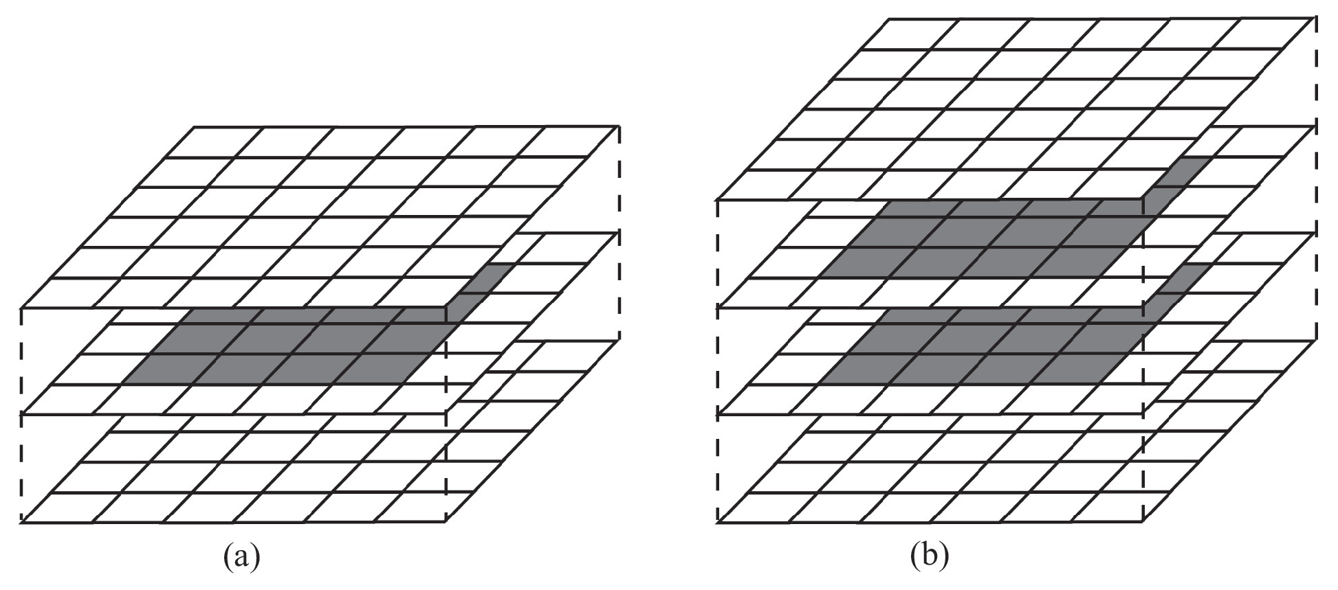
Different data distribution strategies are compared when each thread block is a $4\times 4$ matrix (Figure 15). In Figure 15a, the block is mapped to a subdomain with $4\times 4$ cells (108 cells including 16 computational and 92 ghost cells). To update variables in cells, copies of subdomain and ghost cells are made to the shared memory. To compute variables in $4\times 4$ cells, $6\times 6\times 3$ cells are copied to the shared memory. The block of threads updates less than 15% of shared memory. The breakdown shown in Figure 15b (144 cells including 32 computational cells and 112 ghost cells) allows threads to update variables in cells located in various columns. Each thread updates variables in two cells. The threads work with $4\times 4\times 2$ cells, and the total number of cells is $6\times 6\times 4$. Cells with updated quantities for the requested functions make up 22% of the overall number of cells. The time spent moving data between shared and global memory is compensated for by the increase in computational load per thread.

Based on the computations in [21], the kernel implementations intended to compute preliminary velocity and solve the Poisson equation for pressure are the most important in terms of shared memory utilization. Using shared memory instead of merely global memory can result in performance increases of over two times. The computational load on other kernels is comparatively low.

The scalar product of vectors and matrix-vector operations, which are covered in [2], are implemented in parallel as part of the parallelization of the BiCGStab method. They are implemented using functions from the CUDBLAS library.

14. Multigrid Method

The multigrid approach is used to solve a system of algebraic equations generated by finite volume discretization of the Poisson equation in the projection technique [18].

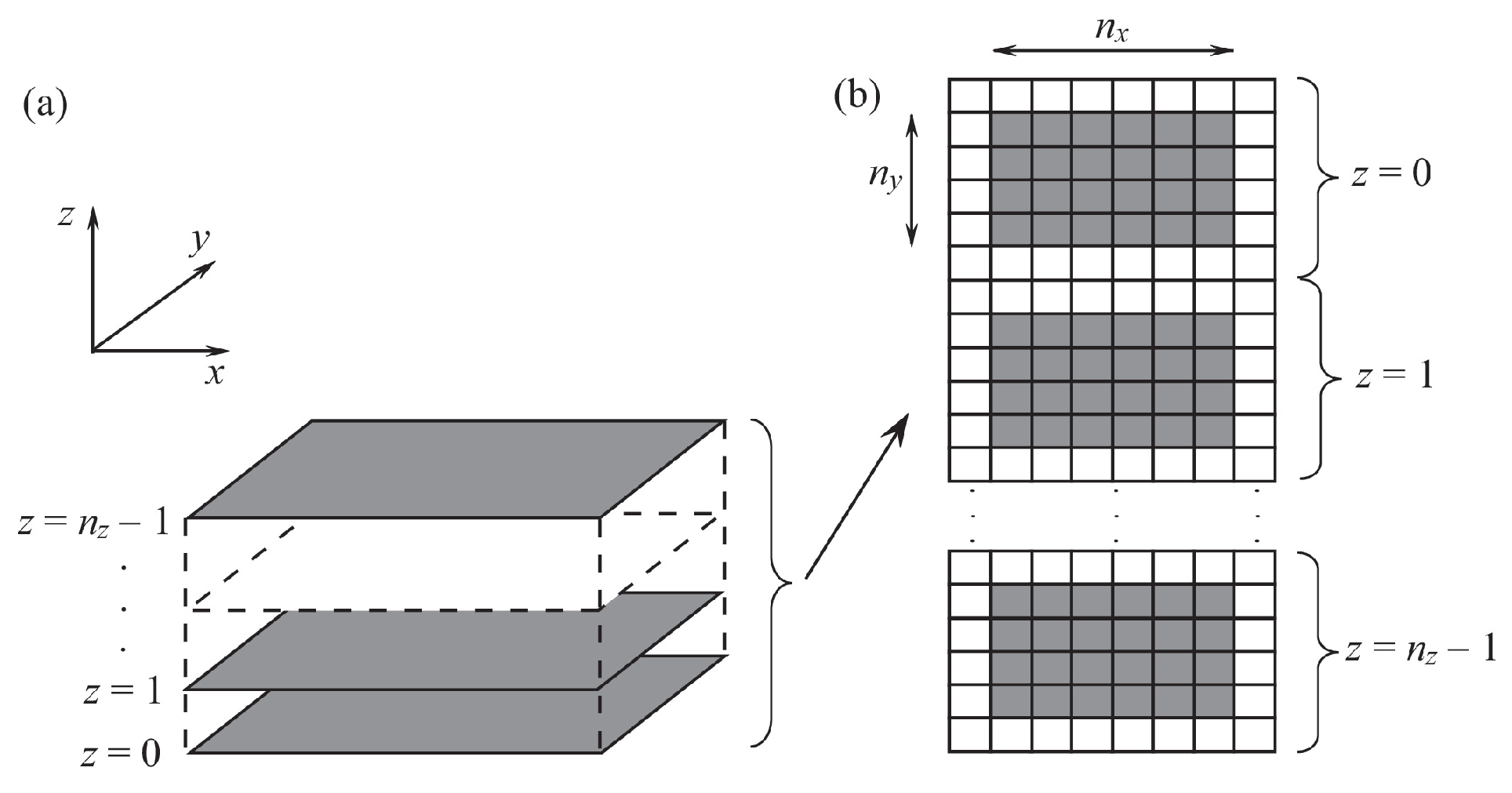
A computational mesh (data array) of dimension $n_x\times n_y\times n_z$ can be mapped onto GPU blocks as seen in Figure 16. n is the number of mesh levels in a system of difference equations that is solved using the multigrid technique. The Gauss–Seidel method with red/black parallelization (V-cycle is utilized) is the smoothing algorithm.

Each thread modifies one data array element and computes parameters in a single cell. The block of threads is three-dimensional, whereas the grid of blocks is two-dimensional. The integer division operation is used to determine the index of each thread after combining the array dimensions in y and z directions.

The interior cells indices have values between $(i,j,k)=(2,2,2)$ and $(i,j,k)=(n_x+1,n_y+1,n_z+1)$. The boundary cells are situated along the $(1,1,1)$ and $(n_x+2,n_y+2,n_z+2)$ planes. The size of the GPU grid is $(g_x,g_y,g_z)$, and the size of each block is $(b_x,b_y,b_z)$. By dividing mesh sizes by block size, GPU grid sizes in $g_x$ and $g_y$ directions are determined such that $g_x=n_x/b_x$ and $g_y=n_y/b_y$. The index of array element on which a thread operates is the same as its three-dimensional index. The $(i,j)$ thread processes the mesh layers in the z direction, processing one cell in each layer, where $s=n_z\left(n\right)/b_z-1$. Multiple cells in a column with fixed indices $(i,j)$ are processed by thread in the k direction. The indices of thread are $(t_x,t_y,t_z)$. Inside the kernel, a loop over mesh layers is used to calculate variables in mesh cells (indices i and j stay fixed). Using an array of size $(g_x,g_y,g_z)$, the boundary conditions are set.

The mesh size determines block size (Figure 16). The ideal block size and grid size are incompatible. For instance, the ideal block size is $32\times 1\times 8$ (block size is greater than grid size), while the coarsest mesh level contains $4\times 4\times 4$ nodes.

The CPU code calls the kernel for a fixed mesh level n and iterates over mesh levels.

    // define fine mesh dimensions of blocks

    #define bx_f 32

    #define by_f 1

    #define bz_f 8

    // define coarse mesh dimensions of blocks

    #define bx_c 4

    #define by_c 4

    #define bz_c 4

    ...

    for (n=1; n<=ngrid; n++){

      // use block size for coarse mesh by default

      bx=bx_c; by=by_c; bz=bz_c;

      // for finer meshes, use better block size

      if (nx[n]%bx_f==0 && ny[n]%by_f==0){

        bx=bx_f; by=by_f; bz=bz_f;

      }

      dim3 block(bx,by,bz);

      dim3 grid(nx[n]/bx,ny[n]/by);

      kernel<<<grid,block>>>(n,...);

    }

    ...

The number of mesh levels being processed is fed into the GPU code, which then makes the required computations.

     __global__ void kernel(n,...){

       // offset thread indices to mesh indices

       // i=tx+2, j=ty+2

       i=threadIdx.x+blockIdx.x*blockDim.x+2;

       j=threadIdx.y+blockIdx.y*blockDim.y+2;

       for (slice=0; slice<=nz[n]/blockDim.z-1; slice++){

         k=threadIdx.z+slice*blockDim.z+2;

         m=i+(j-1)*(nx[n]+2)+

             (k-1)*(nx[n]+2)*(ny[n]+2)+begin[n]-1;

         // kernel computations

         ...

       }

     }

The Gauss–Seidel method is red/black parallelized to boost multigrid computation efficiency on GPU. Two kernels are implemented, processing black and red nodes. The host code running on CPU calls kernels to process black and red nodes and counts mesh levels.

     // go through all V-cycles

     for (icyc=1; icyc<=ncyc; icyc++){

       // downleg of V-cycle

       for (n=ngrid; n>=1; n--){

         // use block size for coarse mesh by default

         bx=bx_c; by=by_c; bz=bz_c;

         // for finer meshes, use better block size

         if (nx[n]%bx_f==0 && ny[n]%by_f==0){

           bx=bx_f; by=by_f; bz=bz_f;

         }

         dim3 block(bx,by,bz);

         dim3 grid(nx[n]/bx,ny[n]/by);

         for (iswp=1; iswp<=nswp; iswp++){

           red_kernel<<<grid,block>>>(n,...);

           black_kernel<<<grid,block>>>(n,...);

         }

       }

     }

The required computations are carried out by the device code, which runs on GPU (the kernels for black and red nodes are implemented similarly).

     __global__ void red_kernel(...){

       i=threadIdx.x+blockIdx.x*blockDim.x+2;

       j=threadIdx.y+blockIdx.y*blockDim.y+2;

       for (slice=0; slice<=nz_d[n]/blockDim.z-1; slice++){

         k=threadIdx.z+slab*blockDim.z+2;

         // test if red cell

         if ((i+j+k)%2==0){

           m=i+(j-1)*(nx[n]+2)+(k-1)*(nx[n]+2)*(ny[n]+2)+begin[n]-1;

           xm=xm[m]; xp=xp[m];

           ym=ym[m]; yp=yp[m];

           zm=zm[m]; zp=zp[m];

           res=(aw_d[m]*pressure_d[xm]+ae_d[m]*pressure_d[xp]+

                as_d[m]*pressure_d[ym]+an_d[m]*pressure_d[yp]+

                al_d[m]*pressure_d[zm]+ah_d[m]*pressure_d[zp]+resc_d[m])/ap_d[m];

           pressure_d[m]=relxp*(res)+(1.0-relxp)*pressure_d[m];

         }

       }

     }

According to calculations, the smoothing process uses the most computer time, accounting for between 72 and 79% of the total calculation time, depending on mesh size. At the same time, less than 8–10% and 12–20% of the total calculation time is needed to implement the continuation and limitation procedures.

15. Flow in a Lid-Driven Cavity

Consideration is given to the unsteady flow of viscous incompressible fluid in the square/cubic cavity caused by the upper wall moving with a constant velocity $U=1$ m/s in the x direction. A cavity has a side of $L=1$ m. The cavity is represented as a mesh $[0,N_1]\times [0,N_2]$ to simulate the flow, with $N_k$ denoting the number of nodes in the k direction.

Reynolds number, $\mathrm{Re}=\rho UL/\mu$, determines flow structure. The cavity side length and upper wall velocity are used to compute the Reynolds number. A fluid with a density of $\rho =1.2\mathrm{kg}/{\mathrm{m}}^3$ and a molecular viscosity that corresponds to a specified Reynolds number is used for the computations (the Reynolds number changes because of a change in the relaxation time). Homogeneous boundary conditions ($v=0$, $p={10}^5$ Pa) are applied at initial time $t=0$. The tangential and normal velocity components on the cavity walls are subject to no-slip and no-flow boundary conditions.

The governing equations are discretized using the projection method [18], and the Smagorinsky model is employed as the subgrid scale (SGS) eddy model. There are ${128}^3$ nodes in the mesh with the highest resolution.

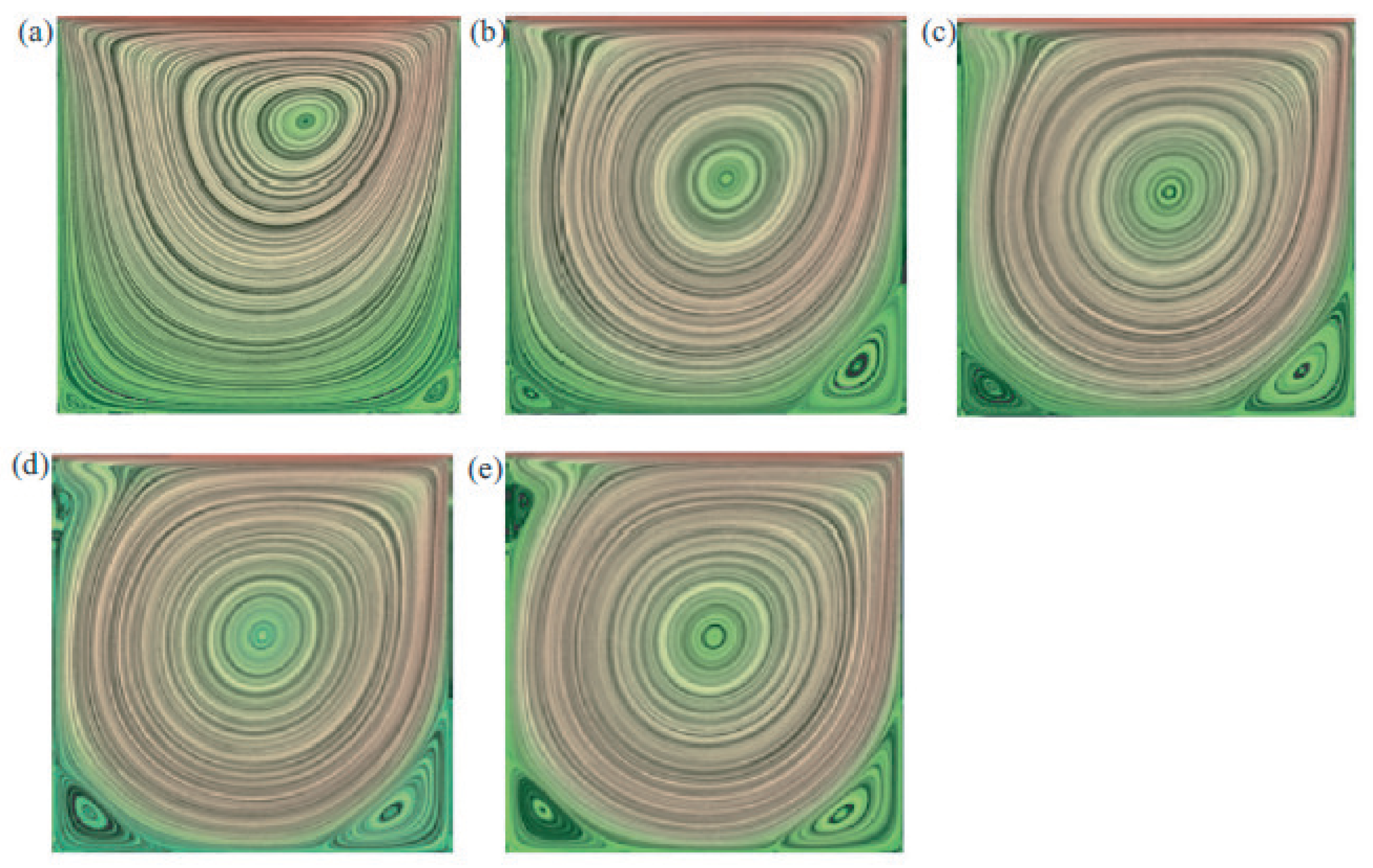
The Reynolds number range for simulating the flow in a square cavity is $\mathrm{Re}=$ 0–5000. The computations make use of meshes with varying resolutions. For various Reynolds numbers, Figure 17 illustrates how the flow field in the cavity is processed using conventional visualization techniques (level lines and color filling).

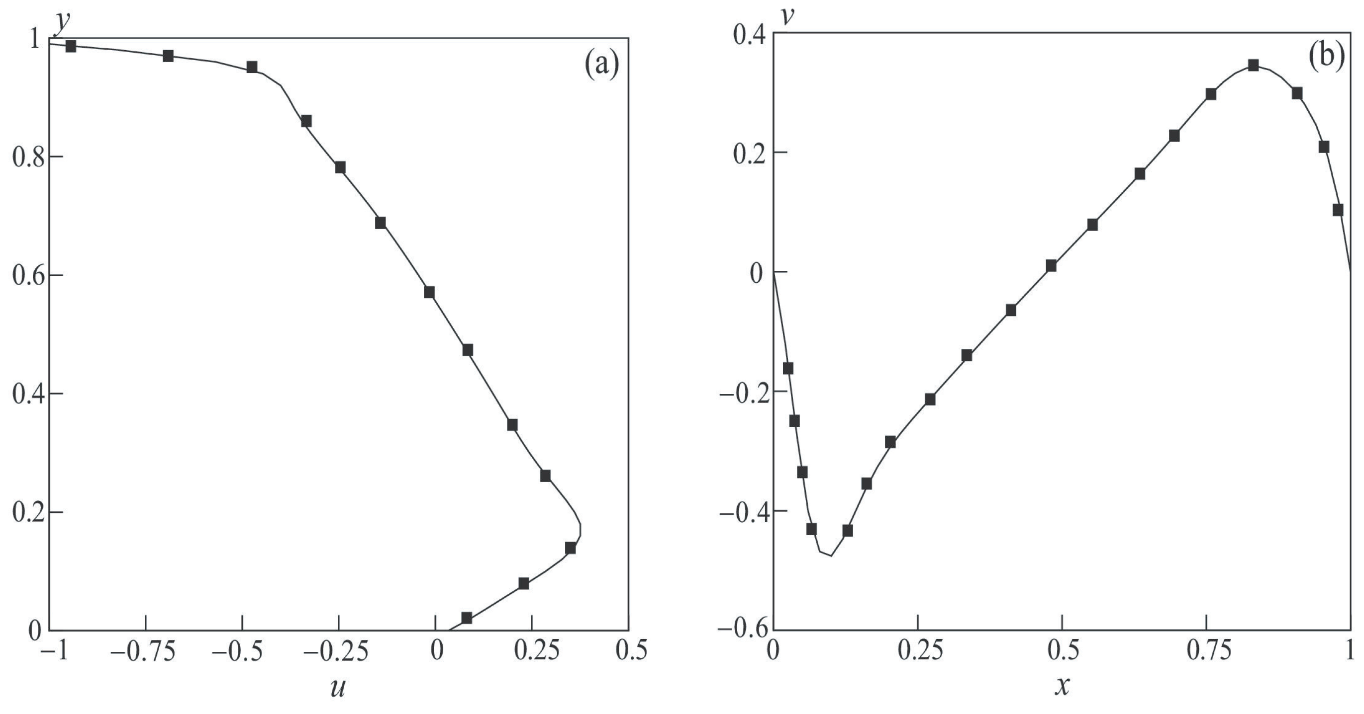
The profiles of longitudinal and transverse velocity components in the mid-section of the cavity are shown in Figure 18 for $\mathrm{Re}=1000$. The calculation results (symbols ◼) are compared with the data of the physical experiment [22] (solid line). The zigzag shape of the longitudinal velocity profile at high Reynolds numbers reflects the process of mixing two flows with different energy characteristics: the non-uniform near-wall flow entrained by the moving wall and the flow circulating in a large-scale vortex.

Estimates of the quality of the numerical solution are based on the positions of primary vortex P, secondary corner vortices L and R close to the stationary lower wall, and stream function at the centers of these vortices.

Table 2. Impact of mesh size on flow calculations in a square cavity at $\mathrm{Re}=100$.

Grid	Vortex P			Vortex L			Vortex R
	${\mathit{x}}_{\mathit{P}}$	${\mathit{y}}_{\mathit{P}}$	${\mathit{\psi }}_{\mathit{m}}$	${\mathit{x}}_{\mathit{L}}$	${\mathit{y}}_{\mathit{L}}$	${\mathit{\psi }}_{\mathit{m}}$	${\mathit{x}}_{\mathit{R}}$	${\mathit{y}}_{\mathit{R}}$	${\mathit{\psi }}_{\mathit{m}}$
${81}^2$	0.6125	0.7375	0.1032	0.0324	0.0365	$-1.22\times {10}^{-6}$	0.9375	0.0641	$-1.00\times {10}^{-5}$
${101}^2$	0.6143	0.7361	0.1034	0.0321	0.0375	$-1.62\times {10}^{-6}$	0.9410	0.0620	$-1.62\times {10}^{-5}$
${129}^2$	0.6172	0.7344	0.1034	0.0313	0.0391	$-1.75\times {10}^{-6}$	0.9453	0.0625	$-1.25\times {10}^{-5}$

presents the outcomes of numerical modeling on various meshes for $\mathrm{Re}=100$. The data of [22] and the numerical modeling results agree well.

Table 3. Impact of Reynolds number on flow calculations in square cavity.

Re	Vortex P			Vortex L			Vortex R			Link
	${\mathit{x}}_{\mathit{P}}$	${\mathit{y}}_{\mathit{P}}$	${\mathit{\psi }}_{\mathit{m}}$	${\mathit{x}}_{\mathit{L}}$	${\mathit{y}}_{\mathit{L}}$	${\mathit{\psi }}_{\mathit{m}}$	${\mathit{x}}_{\mathit{R}}$	${\mathit{y}}_{\mathit{R}}$	${\mathit{\psi }}_{\mathit{m}}$
400	0.5547	0.6055	0.1139	0.0508	0.0469	$-1.42\times {10}^{-5}$	0.8906	0.1250	$-6.42\times {10}^{-4}$	[22]
	0.5608	0.6078	0.1121	0.0549	0.0510	$-1.30\times {10}^{-5}$	0.8902	0.1255	$-6.19\times {10}^{-4}$	[25]
	0.5547	0.6055	0.1113	0.0508	0.0469	$-1.25\times {10}^{-5}$	0.8867	0.1211	$-5.94\times {10}^{-4}$	CFD
1000	0.5313	0.5625	0.1179	0.0859	0.0781	$-2.31\times {10}^{-4}$	0.8594	0.1094	$-1.75\times {10}^{-3}$	[22]
	0.5333	0.5647	0.1178	0.0902	0.0784	$-2.22\times {10}^{-4}$	0.8667	0.1137	$-1.69\times {10}^{-3}$	[25]
	0.5313	0.5664	0.1142	0.0820	0.0742	$-1.84\times {10}^{-4}$	0.8633	0.1094	$-1.60\times {10}^{-3}$	CFD
5000	0.5117	0.5352	0.1190	0.0703	0.1367	$-1.36\times {10}^{-3}$	0.8086	0.0742	$-3.08\times {10}^{-3}$	[22]
	0.5176	0.5373	0.1214	0.0784	0.1373	$-1.35\times {10}^{-3}$	0.8078	0.0745	$-3.03\times {10}^{-3}$	[25]
	0.5156	0.5586	0.1030	0.0781	0.1406	$-1.80\times {10}^{-4}$	0.8086	0.0742	$-2.91\times {10}^{-3}$	CFD

illustrates how Reynolds number affects flow calculations in a square lid-driven cavity. In a wide interval of Reynolds numbers, the CFD results are in good agreement with the reference data [22,23,24,25,26,27,28,29,30,31].

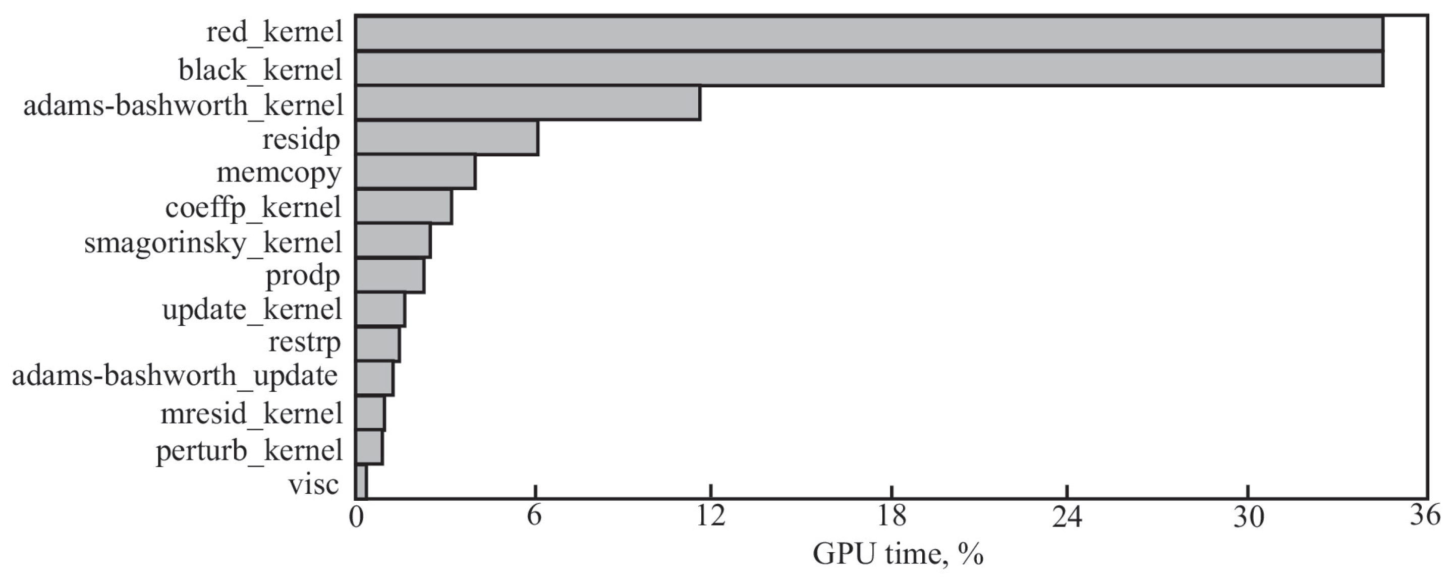
Figure 19 displays the cost of running various code segments. Nearly two-thirds of the computation time is spent on implementing the Gauss–Seidel method with red/black parallelization (routines red_kernel and black_kernel). The discretization of governing equations in time is implemented by the adams_bashworth routine, which is the next most costly routine in terms of processor time. The residual of the Poisson equation is computed by routine residp. The routine memcopy is used to allocate memory and perform copying for variables.

Using the Smagorinsky model, the routines coeffp_kernel and smagorinsky_kernel compute eddy viscosity and coefficients related to the discretization of the Poisson equation. The routines update_kernel and adams_bashworth_kernel are used to move on to the next time layer. Other routines (prodp, restrp, mresid_kernel, perturb_kernel, visc) that carry out unimportant operations contribute comparatively little to the overall computation time.

The calculation speedup when using different meshes and different methods of dividing the domain into blocks of size $n_x\times n_y\times n_z$ is given in

Table 4. Computational time and speedup.

Mesh	Block Size $\mathbf{4}\times \mathbf{4}\times \mathbf{4}$
	CPU, s	GPU, s	Speedup
${16}^3$	0.336	0.392	0.858
${32}^3$	3.084	1.238	2.496
${64}^3$	31.143	6.486	4.805
${128}^3$	291.053	50.923	5.718
Mesh	Block Size $\mathbf{4}\times \mathbf{4}\times \mathbf{4}$
	CPU, s	GPU, s	Speedup
${16}^3$	0.336	0.309	1.11
${32}^3$	3.084	0.657	4.73
${64}^3$	31.143	2.712	11.51
${128}^3$	291.053	18.352	15.88

(the calculation time is given for 100 time steps).

On a mesh containing ${128}^3$ nodes, changing the method of dividing the computational domain into blocks allows us to achieve a gain in speeding up the solution by 2.78 times compared to original division.

Scalability is one of the most critical metrics for evaluating the effectiveness of a GPU-accelerated CFD code. The GPU-accelerated solver is tested. Strong scalability is evaluated on a fixed mesh of 2 million cells, showing a 7.62 speedup from 1 to 8 GPUs (95.3% parallel efficiency). Weak scalability was assessed with a per-GPU cell count of 5 million. The solver maintains more than 90% efficiency up to 64 GPUs across 8 nodes. Data exchange and pressure solver dominate communication time at scale, motivating future overlap and optimization efforts, as well as the development of an algebraic multi-grid (AMG) solver for the Poisson equation.

16. Conclusions

The approaches to solving CFD problems using general-purpose GPUs are considered. The CUDA technology for graphics processors manufactured by NVIDIA is used for software implementation of the code.

The calculation acceleration on meshes with varying resolutions is compared using various techniques for dividing the initial data into blocks. Using a projection method and finite volume method, viscous incompressible fluid flows are simulated. Multigrid method and BiCGStab method are applied to solve the Poisson equation for pressure. Depending on problem formulation and computational algorithms employed, using a GPU can speed up calculations by two to fifty times.