Cross-Dataset Data Augmentation Using UMAP for Deep Learning-Based Wind Speed Prediction

Abstract

Wind energy has emerged as a cornerstone in global efforts to transition to renewable energy, driven by its low environmental impact and significant generation potential. However, the inherent intermittency of wind, influenced by complex and dynamic atmospheric patterns, poses significant challenges for accurate wind speed prediction. Existing approaches, including statistical methods, machine learning, and deep learning, often struggle with limitations such as non-linearity, non-stationarity, computational demands, and the requirement for extensive, high-quality datasets. In response to these challenges, we propose a novel neighborhood preserving cross-dataset data augmentation framework for high-horizon wind speed prediction. The proposed method addresses data variability and dynamic behaviors through three key components: (i) the uniform manifold approximation and projection (UMAP) is employed as a non-linear dimensionality reduction technique to encode local relationships in wind speed time-series data while preserving neighborhood structures, (ii) a localized cross-dataset data augmentation (DA) approach is introduced using UMAP-reduced spaces to enhance data diversity and mitigate variability across datasets, and (iii) recurrent neural networks (RNNs) are trained on the augmented datasets to model temporal dependencies and non-linear patterns effectively. Our framework was evaluated using datasets from diverse geographical locations, including the Argonne Weather Observatory (USA), Chengdu Airport (China), and Beijing Capital International Airport (China). Comparative tests using regression-based measures on RNN, GRU, and LSTM architectures showed that the proposed method was better at improving the accuracy and generalizability of predictions, leading to an average reduction in prediction error. Consequently, our study highlights the potential of integrating advanced dimensionality reduction, data augmentation, and deep learning techniques to address critical challenges in renewable energy forecasting.

1. Introduction

Countries across the world have been compelled to use clean energy technologies due to the increasing demand and the necessity to reduce carbon footprints [1]. Wind energy has gained prominence among many technologies due to its minimum environmental impact and substantial energy production in certain regions [2]. As of 2023, renewable energy possessed an installed capacity of 28,000 GW, of which 600 GW was derived from wind-based sources [3]. Although this represents a substantial contribution, it is rather minor given the pivotal role wind energy is anticipated to assume in the global energy revolution. Regarding this, the Paris Agreement set a goal for renewable energy generation to account for at least 86% of the total by 2050 [4], making the expansion of wind energy capacity essential to meeting these international commitments. However, such a source is directly influenced by the intermittency of weather patterns, which can lead to disruptions in the electrical grid and result in reduced power quality [5].

Additionally, the utilization of wind energy poses specific challenges, particularly in predicting the electricity produced by wind farms. The quantity of energy generated is significantly influenced by wind speed, which is ascertained by a confluence of climatic elements [6]. Specifically, forecasting wind speed presents considerable difficulties owing to the intrinsically non-stationary characteristics of atmospheric patterns, where both short- and long-term variations create complexities that are challenging to quantify [7]. Moreover, the existence of intricate non-linear interactions among meteorological variables exacerbates this challenge [8]. Cyclical events, like El Niño and La Niña, along with their interactions with climate change, produce exogenous conditions that result in randomness and volatility [9].

Conversely, the modeling of wind speed is influenced by the required prediction horizon. Typically, short, medium, high, and high-large horizons are examined. Short-term horizons are essential in turbine control applications, as predictions within one to ten seconds are critical for adjusting the control system in response to wind gusts [10]. Moreover, medium horizons of five to 60 min are beneficial for power grid dispatch and maintenance [11]. In turn, prediction intervals of one to 48 h (high horizons) are utilized for energy trading and power system management [12]. Next, a high-large horizon prediction, which spans from days to years, is crucial for the long-term planning and optimization of wind energy systems. Such predictions enable effective scheduling of maintenance, grid integration, and capacity planning [13].

Now, wind speed forecasting is presently conducted using two separate prediction methodologies: physical-based modeling and data-driven approaches. The initial framework involves a high-large horizon in which functional models are employed. These models feature numerous parameters that characterize on-site weather conditions. Namely, numerical weather predictions (NWPs) are based on the physical processes that govern the transfer of energy and materials within the climate ecosystem [14]. They rely on dynamic physical and thermodynamic principles that clarify interactions between energy and matter across oceans, the atmosphere, and land surfaces. Although they demonstrate high accuracy, their implementation is complicated by the need for extensive parameter tuning and significant computational resources for modeling [15].

On the other hand, data-driven time-series approaches are capable of capturing both stationary and non-stationary patterns in wind speed. Within this category, statistical models, classic machine learning methods, deep learning, and hybrid strategies can be explored [12]. Traditional statistical models encompass auto-regressive with exogenous auto-regressive moving average (ARMA) and auto-regressive integrated moving average (ARIMA), as well as fractional-ARIMA (f-ARIMA). In addition, classical machine learning algorithms were extensively researched because they could find data patterns and provide high interpretability. Some of the most popular methods include Exponential Smoothing (ES) [16], Gaussian Processes (GPs) [17], Ridge Regression [18], Random Forest (RF) [19], and Support Vector Machines (SVMs) [20]. In the third case, deep learning methods have arisen as the most popular machine learning approach to handle non-linear and non-stationary time series due to their ability to extract complex features from input data automatically [21]. Here, models based on memory architectures such as gated recurrent units (GRUs) [22], long short-term memory (LSTM) [11], and attention mechanisms have been employed [23].

Though wind speed approaches have been widely studied, the following issues arise: Statistical models like ARIMA and its variants struggle to effectively model non-linear and non-stationary patterns, limiting their applicability to real-world scenarios with complex dynamics. These methods rely heavily on the assumption of linearity and stationary processes, making them unsuitable for datasets exhibiting abrupt changes or high variability [24]. Next, classical machine learning models, such as SVMs and RF, often require extensive feature engineering, which can be time-consuming and relies heavily on domain expertise. Moreover, despite their high interpretability, these models may fail to capture intricate temporal dependencies inherent in time-series data, leading to suboptimal predictions for highly dynamic wind speed scenarios [25]. In contrast, deep learning methods, while powerful, are computationally expensive and require large datasets for effective training, which may not always be available in wind speed prediction tasks. These models also risk overfitting when applied to small or imbalanced datasets, and their black-box nature limits interpretability, posing challenges for their adoption in operational settings [26]. Hybrid models combining statistical, machine learning, or deep learning approaches may inherit the limitations of their constituent methods and can also be computationally intensive, requiring significant tuning of parameters to achieve a balance between accuracy and complexity [27].

In recent years, enhancing the performance of machine and deep learning models in time-series tasks, i.e., wind speed prediction, has become a critical area of research, driven by the growing reliance on data-driven insights across domains [28]. Although the advancements in model architecture have substantially improved performance, the availability of large, high-quality datasets remains a pivotal factor in enabling effective feature extraction and pattern recognition during the training process. However, real-world applications often face challenges such as limited dataset sizes, poor data quality, and restricted access due to privacy concerns [29]. To address these limitations, strategies like transfer learning (TL) and data augmentation (DA) have emerged as effective solutions. These techniques not only mitigate the constraints of small datasets but also enhance the robustness and generalizability of machine learning models by expanding the diversity of training data [30,31].

In the TL approach, the primary objective is to leverage knowledge representations learned from a source dataset and apply them to a target database. This is especially advantageous when dealing with small sample sets, as it alleviates the need to extract features from scratch, significantly reducing computational overhead and the requirement for extensive labeled data [32]. TL has demonstrated remarkable success across various domains, including image processing [33], where pre-trained models are fine-tuned for specific tasks, and language modeling [34], where embeddings learned from large-scale corpora are adapted for downstream tasks. Regarding wind speed prediction, TL provides pre-trained models or knowledge from related domains to enhance predictive accuracy when datasets are small or region-specific. For instance, models pre-trained on global meteorological datasets can be fine-tuned for specific wind farms, improving localized predictions without requiring extensive labeled data [35]. Recent studies demonstrate the effectiveness of TL in transferring spatial and temporal features from large-scale weather models to wind speed forecasting applications, achieving superior performance compared to models trained solely on limited data [36]. TL techniques, like domain adaptation, have also been used to deal with changes in geography and climate, making wind speed prediction frameworks that are strong and scalable [37]. Nevertheless, the effectiveness of TL is highly dependent on the similarity between the source and target domains; substantial discrepancies in geographical, climatic, or temporal patterns can result in negative transfers, where the adapted model performs worse than a model trained exclusively on the target data [38]. Also, fine-tuning models that have already been trained usually requires a lot of computer power and specialized knowledge to make the adaptation process better, especially for wind speed forecasting tasks that are very complicated. The incapacity of many TL frameworks to generalize across varied wind farm circumstances requires regular model reconfiguration, which is both time-consuming and computationally costly [39].

Conversely, DA focuses on expanding the original dataset to increase its size and diversity, thereby improving model generalization. Traditional DA techniques, prevalent in image processing, typically apply transformations like cropping, scaling, mirroring, color augmentation, or translation to augment data [40]. However, these methods are not directly transferable to time-series data due to their sequential and temporal dependencies. To address this challenge, synthetic data generation techniques have emerged as a robust alternative. Advanced methods such as variational autoencoders (VAEs) [41] and generative adversarial networks (GANs) [42] have been increasingly employed for time-series augmentation. VAEs encode input data into a probabilistic latent space, enabling the generation of diverse yet realistic data samples. GANs, on the other hand, use a dynamic adversarial process between a generator network and a discriminator network to create high-quality synthetic data that mirror the statistical properties of the original dataset. These approaches have proven particularly beneficial in applications such as wind speed prediction, where the availability of extensive, high-quality time-series data are often limited. For example, GAN-based DA methods have been used to improve wind speed datasets, which has led to more accurate short-term forecasts by creating more realistic synthetic samples [43]. Similarly, hybrid models leveraging DA techniques have demonstrated enhanced performance in predicting extreme wind speed events, where original datasets are sparse or highly imbalanced [44]. Still, DA methods often have trouble keeping the temporal and sequential integrity of the wind speed time series. This can cause problems with the synthetic data that are generated, which can hurt the performance of the model [45]. Additionally, the computational cost and complexity of advanced DA methods, such as GANs and VAEs, can pose significant challenges when processing large-scale datasets [46]. Lastly, variability across different datasets (region-specific wind speed prediction) decreases the DA’s performance [47].

In this study, we propose a novel neighborhood preserving cross-dataset data augmentation approach tailored for deep learning-based wind speed prediction in high-horizon scenarios. We have designed our method to tackle the issues of data variability and dynamic behavior that frequently arise in wind speed forecasting. Specifically, our approach comprises three key components:

• We use the uniform manifold approximation and projection (UMAP) [48] as a non-linear dimensionality reduction algorithm to find and encode local relationships in wind speed time-series samples. The low-dimensional representation of the data preserves its neighborhood structures.
• A localized cross-dataset DA approach is introduced from the UMAP-reduced spaces, which leverages localized neighborhoods to mitigate data variability across multiple wind speed datasets, enhancing the diversity and robustness of the augmented training data [47].
• Recurrent neural networks (RNNs) are trained using the augmented datasets, capitalizing on their ability to model temporal dependencies and non-linear patterns in wind speed time-series data.

Our framework improves the generalization capability of predictive models by exposing them to a wide range of conditions and behavioral patterns. Experiments include wind speed time series from weather stations at the Argonne Weather Observatory in Illinois, USA; the Chengdu Airport in Sichuan Province, China; and the Beijing Capital International Airport, China. Additionally, the method comparison comprises the straightforward RNN, GRU, and LSTM architectures using regression-based quantitative assessments. Thus, our approach is a promising alternative for wind-based energy monitoring.

The reminder of this paper is organized as follows: Section 2 describes the materials and methods. Section 3 and Section 4 describe the experimental set-up and obtained results. Finally, the conclusions are outlined in Section 5.

2. Materials and Methods

2.1. Wind Speed Time-Series Datasets

We utilized three distinct datasets for wind speed prediction collected from meteorological stations. The key characteristics of each dataset are detailed below, including the recording period, sensor specifications, geographic location, regional climate conditions, dataset size, and the properties of the available measurements.

Argonne. The first dataset originates from the Argonne Weather Observatory, located at the Argonne National Laboratory in Illinois, west of Chicago, in the Midwestern United States (see https://pubs.usgs.gov/wdr/2005/wdr-il-05/data/wind_por/indices0/index.htm) (accessed on 1 January 2025). Geographically, the observatory is positioned at 41° N latitude and 87° W longitude. Wind speed data were recorded over an extensive period, spanning from 1 January 1998 to 30 August 2005, with an hourly sampling frequency. The Argonne dataset, encompassing more than five decades of observations, offers a comprehensive record with hundreds of thousands of data points, capturing a wide range of wind speed variations and providing valuable insights into long-term atmospheric dynamics. Wind speed measurements were taken using Met One Instruments Model 10B anemometers. Additional meteorological variables, including temperature, humidity, and solar radiation, were recorded with high-precision sensors such as the Vaisala HMP45A (temperature and dewpoint) and the Eppley pyranometer (solar radiation). The Argonne station has been in continuous operation since 1948, with rigorous data correction processes ensuring reliability. The region experiences a continental climate, featuring cold winters, mild summers, and distinct seasonal transitions.

Chengdu. The second dataset originates from Chengdu Airport in Sichuan Province, China, at coordinates 30.6° N latitude and 104.01° E longitude (see https://mesonet.agron.iastate.edu/request/download.phtml?network=PK__ASOS) (accessed on 1 January 2025). Covering nearly eight years, from 1 January 2011 to 30 December 2018, with hourly observations, it provides tens of thousands of data points. Situated in a subtropical monsoon climate, Chengdu experiences mild winters, warm, humid summers, and concentrated summer rainfall. The Sichuan Basin’s unique geography contributes to frequent fog and high humidity, which can affect wind measurements. Although details of the anemometer model are unavailable, the dataset adheres to China’s ASOS standards, ensuring high-quality data. This dataset complements the Argonne dataset by offering insights into wind dynamics under monsoon climates and complex topographical influences.

Beijing. The third dataset is sourced from Beijing Capital International Airport, located at 39.9° N latitude and 116.2° E longitude (see https://talltowers.bsc.es) (accessed on 1 January 2025). As a climatological and synoptic station under the Global Basic Observing Network (GBON) and the World Meteorological Organization (WMO), it provides high-quality data. For this study, wind speed measurements from 1 August 2011 to 30 December 2018, were used, offering tens of thousands of hourly observations. Beijing’s continental monsoon climate, with cold, dry winters and hot, humid summers, drives significant seasonal wind speed variations influenced by temperature and atmospheric pressure shifts. The dataset offers a unique perspective compared to Chengdu and Argonne, capturing a distinct climate regime.

The three datasets together form a robust resource for analyzing wind speed dynamics across varied climatic and geographical settings. By encompassing continental, monsoon, and subtropical monsoon climates, they provide a comprehensive foundation for assessing the generalizability and performance of wind speed prediction approaches.

Table 1. Wind speed datasets main statistical description. Std.: Standard Deviation.

Dataset	Start	End	Max	Mean	Min	Median	Std.
Argone	1 January 1998	30 August 2005	32.44	7.28	0	6.49	3.83
Chengdu	1 January 2011	30 December 2018	33.53	3.52	0	2.24	2.95
Beijing	1 August 2011	30 December 2018	40.23	6.48	0	4.47	4.85

and Figure 1 illustrate the statistical description and the geographical distribution of the studied databases.

2.2. Uniform Manifold Approximation and Projection (UMAP)

UMAP is a powerful tool for dimensionality reductions, well suited for capturing non-linear relationships in high-dimensional datasets. By preserving both global and local structures, UMAP outperforms many traditional methods, offering meaningful low-dimensional embeddings that reflect the underlying data geometry. Compared to techniques like principal component analysis (PCA) and t-distributed stochastic neighbor embedding (t-SNE), UMAP excels in balancing computational efficiency with the ability to maintain meaningful neighborhood relationships, making it particularly effective for clustering and visualization tasks [49]. These strengths make UMAP an ideal choice for tasks requiring the reduction of complex, non-linear data while preserving key structural properties essential for further prediction stages.

Here, given a high-dimensional input matrix $\mathbf{X}\in {\mathbb{R}}^{N\times \tau }$, which contains N wind speed time-series segments across $\tau$ time instants, UMAP seeks to compute a low-dimensional embedding $\mathbf{Z}\in {\mathbb{R}}^{N\times M}$, with $M\le \tau$ low-dimensional features. This embedding is designed to preserve both the global and local neighborhood structures present in $\mathbf{X}$, thereby maintaining the key non-linear relationships inherent in the data. To achieve this, UMAP constructs a K-nearest neighbor (KNN) graph as

$${\theta }_n=\underset{{\mathbf{x}}_{n^{\prime }}\in {\Omega }_n}{min}\mathrm{d}({\mathbf{x}}_n,{\mathbf{x}}_{n^{\prime }}),$$

(1)

where $\mathrm{d}(·,·)\in {\mathbb{R}}^{+}$ is the Euclidean distance function, ${\theta }_n\in {\mathbb{R}}^{+}$ holds the minimum distance within the n-th neighborhood, and ${\Omega }_n\in {\mathbb{R}}^{K\times \tau }$ holds K neighbors ${\mathbf{x}}_{n^{\prime }}\in {\mathbb{R}}^{\tau }$ centered on ${\mathbf{x}}_n\in {\mathbb{R}}^{\tau }$. Next, a localized entropy ${\xi }_n\in {\mathbb{R}}^{+}$ is computed for each input segment by solving

$$\sum _{n^{\prime }=1}^{K}exp\left(-{\displaystyle \frac{\mathrm{d}({\mathbf{x}}_n,{\mathbf{x}}_{n^{\prime }})-{\theta }_n}{{\xi }_n}}\right)=log\left(K\right).$$

(2)

Subsequently, UMAP constructs a fuzzy simplicial complex graph, denoted as $\mathcal{G}=(\mathbf{X},\mathbf{A})$, where the edges are determined by local connectivity. The weights of these edges are represented in the matrix $\mathbf{A}\in {[0,1]}^{N\times N}$:

$$a_{n{n}^{\prime }}=exp\left(-max\left(0,{\displaystyle \frac{\mathrm{d}({\mathbf{x}}_n,{\mathbf{x}}_{n^{\prime }})-{\theta }_n}{{\xi }_n}}\right)\right).$$

(3)

In turn, a low-dimensional weight matrix $\tilde{\mathbf{A}}\in {[0,1]}^{N\times N}$ is computed as

$${\tilde{a}}_{n{n}^{\prime }}={\left(1+\alpha \mathrm{d}{({\mathbf{z}}_n,{\mathbf{z}}_{n^{\prime }})}^2\right)}^{-\iota },$$

(4)

where ${\mathbf{z}}_n,{\mathbf{z}}_{n^{\prime }}\in \mathbf{Z}$ represent points in the low-dimensional embedding, while $\alpha ,\iota \in {\mathbb{R}}^{+}$ hyper-parameters (commonly set to 1) balance the preservation of local and global structures. The UMAP optimization problem can then be expressed using a cross-entropy loss function as follows:

$${\mathbf{Z}}^{*}=arg\underset{{\mathbf{z}}_n\in \mathbf{Z}}{min}\sum _{\begin{array}{c}n\in N\\ n\ne n^{\prime }\end{array}}{a}_{n{n}^{\prime }}log\left({\displaystyle \frac{a_{n{n}^{\prime }}}{{\tilde{a}}_{n{n}^{\prime }}\left(\mathbf{Z}\right)}}\right)+\left(1-a_{n{n}^{\prime }}\right)log\left({\displaystyle \frac{1-a_{n{n}^{\prime }}}{1-{\tilde{a}}_{n{n}^{\prime }}\left(\mathbf{Z}\right)}}\right).$$

(5)

Notation ${\tilde{a}}_{n{n}^{\prime }}\left(\mathbf{Z}\right)$ emphasizes the dependency between the low-dimensional embedding $\mathbf{Z}$ and the graph weights in $\tilde{\mathbf{A}}$. Notably, the optimization problem in Equation (5) balances attraction (first term) and repulsion (second term) forces by minimizing the differences between probabilities, represented by the graph weights. Lastly, this optimization can be effectively solved using gradient descent-based methods [48].

2.3. UMAP-Based Cross-Dataset Data Augmentation

Now, let $\mathcal{D}={\{{\mathbf{X}}^r\in {\mathbb{R}}^{N_r\times \tau },{\mathbf{Y}}^r\in {\mathbb{R}}^{N_r\times {\tau }^{\prime }}\}}_{r=1}^R$ represent a multi-region wind speed time-series dataset, where ${\mathbf{X}}^r$ contains $N_r$ input segments spanning $\tau$ time instants and ${\mathbf{Y}}^r$ corresponds to the subsequent ${\tau }^{\prime }$ outputs. Namely, $\mathcal{D}$ encompasses R geographical regions. Here, to capture data variability and non-linear relationships among samples, we propose a cross-dataset DA approach leveraging UMAP-based embeddings.

Regarding this, the augmented input matrix $\tilde{\mathbf{X}}\in {\mathbb{R}}^{\tilde{N}\times \tau }$ is constructed through a row-wise concatenation of the multi-region wind speed time series from $\mathcal{D}$, with $N={\sum }_{r=1}^R{N}_r$. Subsequently, a 2D low-dimensional embedding matrix $\tilde{\mathbf{Z}}\in {\mathbb{R}}^{\tilde{N}\times 2}$ is obtained by solving the optimization problem defined in Equation (5), with the input matrix $\tilde{\mathbf{X}}$ being fixed, as follows:

$$\tilde{\mathbf{Z}}=\mathrm{UMAP}\left(\tilde{\mathbf{X}}\right).$$

(6)

The latter aims to preserve diverse temporal dynamics and regional wind speed characteristics within a neighborhood-based representation. Next, the augmented input–output wind speed time-series data for each r-th region, denoted as ${\widehat{\mathbf{X}}}^r\in {\mathbb{R}}^{{\tilde{N}}_r\times \tau }$ and ${\widehat{\mathbf{Y}}}^r\in {\mathbb{R}}^{{\tilde{N}}_r\times {\tau }^{\prime }}$, is constructed as follows:

$$\begin{array}{cc}\hfill {\widehat{\mathbf{X}}}^r=& {\mathbf{X}}^r\cup \{{\mathbf{x}}_{n^{\prime }}^{r^{\prime }}: \parallel {\tilde{\mathbf{z}}}_{n^{\prime }}^{r^{\prime }}-{\tilde{\mathbf{z}}}_n^r{\parallel }_2 < \zeta ,r^{\prime }\ne r,{\tilde{\mathbf{z}}}_{n^{\prime }}^{r^{\prime }}\notin \Omega \left({\tilde{\mathbf{z}}}_n^r\right)\},\hfill \end{array}$$

(7)

$$\begin{array}{cc}\hfill {\widehat{\mathbf{Y}}}^r=& {\mathbf{Y}}^r\cup \{{\mathit{y}}_{n^{\prime }}^{r^{\prime }}: \parallel {\tilde{\mathbf{z}}}_{n^{\prime }}^{r^{\prime }}-{\tilde{\mathbf{z}}}_n^r{\parallel }_2 < \zeta ,r^{\prime }\ne r,{\tilde{\mathbf{z}}}_{n^{\prime }}^{r^{\prime }}\notin \Omega \left({\tilde{\mathbf{z}}}_n^r\right)\};\hfill \end{array}$$

(8)

where ${\mathbf{x}}_{n^{\prime }}^{r^{\prime }}\in {\mathbf{X}}^{r^{\prime }}$ is the $n^{\prime }$-th augmented sample from the geographical region $r^{\prime }$ related to the low-dimensional neighbor ${\tilde{\mathbf{z}}}_{n^{\prime }}^{r^{\prime }}$ centered on ${\tilde{\mathbf{z}}}_n^r$, with ${\tilde{\mathbf{z}}}_{n^{\prime }}^r,{\tilde{\mathbf{z}}}_n^{r^{\prime }}\in \tilde{\mathbf{Z}}$, $n\in \{1,2,\cdots ,N_r\}$, $n^{\prime }\in \{1,2,\cdots ,N_{r^{\prime }}\}$, and $r,r^{\prime }\in \{1,2,\cdots ,R\}$. Notation ${\tilde{\mathbf{z}}}_{n^{\prime }}^{r^{\prime }}\notin \Omega \left({\tilde{\mathbf{z}}}_n^r\right)$ ensures that neighborhood-based augmentation remains disjoint across datasets, with $\Omega \left({\tilde{\mathbf{z}}}_n^r\right)$ being the UMAP-based data augmentation neighborhood on ${\tilde{\mathbf{z}}}_n^r$.

The hyper-parameter $\zeta \in {\mathbb{R}}^{+}$ rules the low-dimensional neighborhood radius for our UMAP-based cross-dataset data augmentation (UMAP-CDDA). By constructing a unified embedding matrix $\tilde{\mathbf{Z}}$, our method preserves temporal dynamics and regional characteristics while capturing non-linear relationships within multi-region datasets. Namely, through neighborhood augmentation, localized patterns from similar wind speed dynamics are integrated into the training data, improving diversity and mitigating the limitations of small or region-specific datasets.

2.4. Deep Learning-Based Wind Speed Predictions

For each cross-dataset DA pair ${\widehat{\mathbf{X}}}^r$ and ${\widehat{\mathbf{Y}}}^r$, a DL-based algorithm can be trained for wind speed prediction, as follows:

$${\breve{\mathbf{Y}}}^r=\tilde{\varsigma }({\widehat{\mathbf{X}}}^r|\nu )=({\varsigma }_L\circ {\varsigma }_{L-1}\circ \cdots \circ {\varsigma }_1)({\widehat{\mathbf{X}}}^r),$$

(9)

Notation ∘ stands for function composition. ${\breve{\mathbf{Y}}}^r\in {\mathbb{R}}^{{\tilde{N}}_r\times {\tau }^{\prime }}$ holds the wind speed predictions, L stands for the number of layers, and

$${\mathit{F}}_l={\varsigma }_l\left({\mathit{F}}_{l-1}\right)=\sigma ({\mathit{F}}_{l-1}\otimes {\mathit{\varpi }}_l+{\mathit{\beta }}_l),$$

(10)

where $\sigma (·)$ is a non-linear activation, ${\mathit{F}}_l$ is the l-th feature map, ${\mathit{\varpi }}_l$ and ${\mathit{\beta }}_l$ hold the weights and bias of proper size, and $\nu ={\{{\mathit{\varpi }}_l,{\mathit{\beta }}_l\}}_{l=1}^L$ gathers the network parameters. Furthermore, ⊗ represents the tensor product operator for recurrent layers. In this study, three well-known recurrent layers are considered:

–

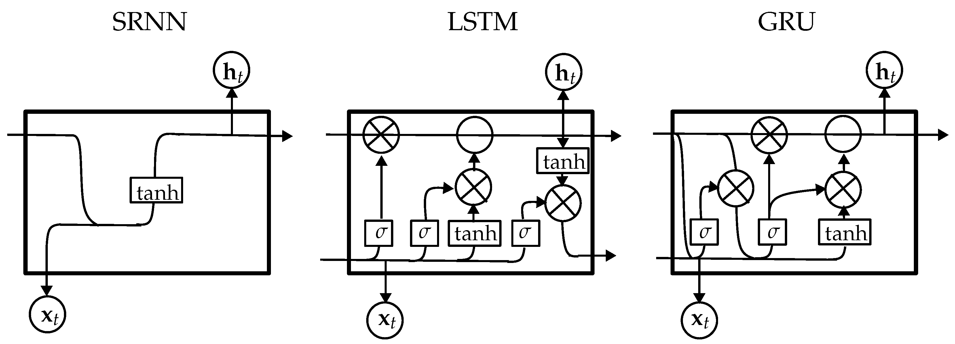
Simple recurrent neural networks (SRNNs) are a foundational deep learning architecture designed to model sequential data by capturing temporal dependencies. RNNs process the augmented data generated by the UMAP-based cross-dataset approach. In short, the RNN architecture iteratively processes the input sequences, maintaining a hidden state that carries information from previous time steps, enabling the network to learn patterns and trends over time [50].

–

Long short-term memory (LSTM) networks are an advanced architecture specifically designed to overcome the limitations of SRNNs, such as vanishing or exploding gradients, when modeling long-range temporal dependencies. The LSTM architecture introduces memory cells and gating mechanisms—input, forget, and output gates—that enable the selective retention and propagation of relevant information over extended time sequences. This allows for effectively capturing the temporal dynamics and complex non-linear data patterns [35].

–

Gated recurrent units (GRUs) are a simplified but powerful variant of LSTM networks, designed to efficiently model sequential data by capturing temporal dependencies with reduced computational complexity. GRUs utilize gating mechanisms—update and reset gates—to regulate the flow of information, enabling the network to retain or discard information dynamically over time. This design allows GRUs to learn complex temporal patterns while maintaining a lighter computational footprint compared to LSTMs [51]. Figure 2 summarizes the main SRNN, LSTM, and GRU layers.

Then, the following optimization arises:

$${\nu }^{*}=arg\underset{\nu }{min}{\displaystyle \frac{1}{N_r}}\sum _{n=1}^{N_r}\mathcal{L}({\mathit{y}}_n^r,{\breve{y}}_n^r),$$

(11)

where ${\breve{y}}_n^r=\tilde{\varsigma }({\widehat{\mathbf{x}}}_n^r|\nu )$, ${\widehat{\mathbf{x}}}_n^r\in {\widehat{\mathbf{X}}}^r$, and $\mathcal{L}(·,·)$ is a given loss function. A backpropagation-driven gradient descent framework is utilized to optimize the parameter set [50]:

$${\nu }_i={\nu }_{i-1}-{\eta }_i{\displaystyle \frac{\partial }{\partial {\nu }_{i-1}}}\left\{{\displaystyle \frac{1}{N_r}}\sum _{n=1}^{N_r}\mathcal{L}({\mathit{y}}_n^r,{\breve{y}}_n^r)\right\}.$$

(12)

An approach based on automatic differentiation computes the gradient, where ${\eta }_i\in {\mathbb{R}}^{+}$ represents the learning rate. Here, the following kernel-based mean square error (KMSE) loss function is employed [52]:

$$KMSE(\mathit{y},\breve{\mathit{y}})={\displaystyle \frac{1}{{\tau }^{\prime }}}\sum _{t=1}^{{\tau }^{\prime }}exp\left({\displaystyle \frac{-\parallel y_t-{\breve{y}}_t{\parallel }_2^2}{2{\breve{\sigma }}^2}}\right),$$

(13)

where $\breve{\sigma }\in {\mathbb{R}}^{+}$ serves as a bandwidth hyper-parameter that regulates the discrepancy between target and network prediction and ${\parallel ·\parallel }_2$ stands for the l2-norm operator.

3. Experimental Set-Up

We used the three wind speed datasets from Section 2.1 for real-world testing. Data were split into training sets (80%) and testing sets (20%). The training period for the Argonne dataset spanned from 1998-01-01 01:00 to 1994-03-14 10:00, while testing covered 1994-03-14 11:00 to 2005-09-30 24:00. For the Chengdu dataset, training data ranged from 2011-08-01 00:00 to 2017-07-07 16:00, with testing from 2017-07-07 17:00 to 2018-12-29 23:00. Similarly, the Beijing dataset’s training period extended from 2011-01-01 00:00 to 2017-05-27 15:00, and testing spanned 2017-05-27 15:00 to 2018-12-29 23:00. To find temporal dependencies, we used windowing with a single-sample shift to make sure there was the most overlap and that the sequence stayed the same. This enhances feature extraction and model generalization, which is crucial for accurate forecasting [53].

In the training phase, hold-out validation was used. For concrete testing, the input window size and the horizon values are fixed as $\tau =20$ and ${\tau }^{\prime }\in \{1,2,\cdots ,7\}$ hours, as a suitable range for energy planning applications [54]. Similarly, the radius is chosen from $\zeta \in \{0.0,0.01,0.02,0.05,0.07,0.01,0.02\}$. This selection process maintains a balance between computational efficiency and predictive accuracy by optimizing the resolution of the tested hyper-parameters. Also, we set the UMAP neighborhood size to 50, enhancing the preservation of fine-grained local structures, making the embedding highly sensitive to small-scale variations. Minimal local connectivity, ${\theta }_n=1$, enforces strong separation between clusters by limiting the number of strongly connected neighbors. Before processing data with recurrent architectures and the proposed UMAP-CDDA, a preprocessing stage encompassing min–max normalization between 0 and 1 is applied to enhance numerical stability and convergence [55]. Figure 3 summarizes our UMAP-CDDA-based training pipeline for predicting wind speed time series.

The mean absolute error (MAE), the mean absolute percentage error (MAPE), and the $R^2$ score are used as quantitative assessment measures [56]:

$$MAE(\mathit{y},\breve{\mathit{y}})={\displaystyle \frac{1}{{\tau }^{\prime }}}\sum _{t=1}^{{\tau }^{\prime }}{\parallel y_t-{\breve{y}}_t\parallel }_1,$$

(14)

$$MAPE(\mathit{y},\breve{\mathit{y}})={\displaystyle \frac{1}{{\tau }^{\prime }}}\sum _{t=1}^{{\tau }^{\prime }}{\displaystyle \frac{\parallel y_t-{\breve{y}}_t{\parallel }_1}{\parallel y_t{\parallel }_1}},$$

(15)

$$R^2(\mathit{y},\breve{\mathit{y}})=1-{\displaystyle \frac{{\sum }_{t=1}^{{\tau }^{\prime }}{\parallel y_t-{\breve{y}}_t\parallel }_2^2}{{\sum }_{t=1}^{{\tau }^{\prime }}{\parallel y_t-\overline{y}\parallel }_2^2}},$$

(16)

where ${\parallel ·\parallel }_2$ and ${\parallel ·\parallel }_1$ stand for the l1- and l2-based norm operators. Also, $\overline{y}={\displaystyle \frac{1}{{\tau }^{\prime }}}{\sum }_{t=1}^{{\tau }^{\prime }}{y}_t$. Here, $R^2$ values lower than 0 are set to 0.

To evaluate the effectiveness of our UMAP-CDDA approach, we compared it against a straightforward recurrent network incorporating SRNN, LSTM, and GRU layers, using the KMSE in Equation (13) as the loss function with $\breve{\sigma }=\sqrt{2}/2$. The comparison was conducted with and without our data augmentation strategy while maintaining the same architecture (see

Table 2. DL main architecture for UMAP-CDDA-based wind speed prediction. $\tau$ represents the input window size and ${\tau }^{\prime }$ the prediction horizon ($\tau =20$ and ${\tau }^{\prime }=7$ h/samples in our experiments). $h=9$ Units are fixed for the recurrent layer.

Layer	Output Dimension
Input	$1\times \tau$
Recurrent (Activation: ReLU)	$1\times h$
SRNN/GRU/LSTM
Dense (Activation: Linear)	$1\times {\tau }^{\prime }$

) [52].

The UMAP-CDDA optimization process runs for 100 epochs, ensuring a balance between computational efficiency and embedding stability. Also, to compute UMAP on large datasets, we leverage the RAPIDS cuML package https://docs.rapids.ai/api/, (accessed on 1 December 2024) version 24.10.0, which utilizes GPU acceleration for significantly faster execution compared to CPU-based implementations. This approach improves scalability, enabling the processing of datasets with millions of points while maintaining low latency.

Next, we trained each DL model using TensorFlow version 2.17.0 and Keras version 3.2.1. All tests were performed in Kaggle notebook environments. These environments provide two Tesla T4 GPUs with 15GB of VRAM, 30GB of RAM, an Intel Xeon CPU @ 2GHz with two threads per core, and two sockets per core. We set a maximum of 100 epochs, a learning rate of 1 × 10⁻³, and an Adam optimizer. All notebooks and codes are publicly available at https://github.com/ealeongomez/UMAPCDDA (accessed on 1 December 2024).

4. Results and Discussion

4.1. UMAP-CDDA Visual Inspection Results

Figure 4 depicts the UMAP-based dimensionality reduction plots, where each point represents a reduced representation of an input window with $\tau =20$ h. The color of each point corresponds to the average output wind speed for the following ${\tau }^{\prime }=7$ horizon points (hours), as indicated by the color bar. This visualization enables an analysis of the dispersion of wind speed values within each dataset. When examining the datasets individually, the Argonne samples demonstrate a well-clustered and consistent distribution of input windows across input samples. Similarly, the Beijing dataset exhibits a structured dispersion of wind speed, though with a wider spread of points. This evidence suggests that while there is some structure in the data, the relationship between input windows and predicted outputs is less robust, leading to greater variability in predictions. In contrast, the Chengdu dataset presents different behavior. The clustering pattern is less distinct compared to the Argonne and Beijing datasets, with points appearing more widely dispersed. This lack of clear separation between wind speed values may be attributed to the complex characteristics of the Chengdu time series, where non-linear dependencies and dynamic meteorological conditions introduce greater variability. As a result, it exhibits more overlap between different wind speed ranges, making it difficult to distinguish distinct patterns in the low-dimensional representation.

Overall, the UMAP-based 2D representation highlights the influence of dataset-specific characteristics on wind speed relationships, where structured patterns emerge in some datasets (Argonne and Beijing), while increased complexity in the time series (as seen in Chengdu) can obscure the separation of wind speed values. Figure 5 shows the UMAP low-dimensional representation of the combined datasets. The left plot uses color to represent the average speed along the horizon (${\tau }^{\prime }=7$), while the right figure shows the membership of each input dataset (Argonne, Beijing, or Chengdu). By comparing both visualizations, it is possible to analyze the effectiveness of the neighborhood-based augmentation process. The overlap between different datasets in the right panel highlights the potential for cross-dataset data augmentation, where similar wind speed patterns across locations enhance the richness of the training set. As the neighborhood radius expands, a greater number of samples from diverse datasets are integrated into the augmentation process, increasing variability and improving model generalization. However, an excessively large radius may introduce undesirable noise, blending distinct wind regimes and diminishing the specificity of localized wind speed characteristics. Therefore, carefully selecting an optimal neighborhood radius is essential to striking a balance between enhancing data diversity and preserving meaningful patterns critical for accurate modeling.

Moreover, Figure 6 and Figure 7 depict the distribution of the DA samples and the percentage increase as the radius of the neighborhood (threshold) increases. In the Argonne dataset, the augmentation rate initially grows steadily, reflecting the relatively homogeneous nature of its wind speed patterns. However, at higher threshold values, the growth rate stabilizes, suggesting that additional augmentation provides diminishing returns. In contrast, the Beijing dataset exhibits a more pronounced increase in DA, particularly at mid-range threshold values, indicating a greater diversity in wind speed patterns. The latter behavior suggests that Beijing’s dataset contains more complex and varied temporal structures that benefit significantly from neighborhood expansion. Lastly, the Chengdu database shows the lowest DA percentage. This can be attributed to the dataset’s highly variable wind speed patterns, influenced by the region’s monsoon climate and frequent atmospheric fluctuations. Then, Chengdu data points are less densely clustered in the UMAP space, leading to a lower incorporation of cross-dataset samples from neighboring regions.

4.2. Wind Speed Prediction Method Comparison Results

Figure 8 presents the wind speed prediction outcomes, measured by MAE, MAPE, and $R^2$, in relation to the UMAP-CDDA radius and prediction horizon. The results compare baseline deep learning models—SRNN, GRU, and LSTM—without data augmentation ($\zeta =0$) against our CDDA-enhanced approach ($\zeta >0$). As shown, the baseline models exhibit moderate to strong predictive performance for the Argonne and Beijing datasets, particularly with LSTM and GRU. However, introducing data augmentation at low thresholds (0.01–0.05) yields notable improvements, suggesting that incorporating cross-dataset samples enhances generalization by better capturing local wind dynamics. In contrast, the Chengdu dataset initially struggles with weak predictive performance at lower thresholds, indicating poor model generalization. Yet, as the augmentation threshold increases (0.02–0.05), a significant performance boost emerges, underscoring the effectiveness of the augmentation process in mitigating initial weaknesses and reinforcing model adaptability. Notably, the most significant enhancements are seen in LSTM and GRU models, which appear to benefit the most from augmented data, as their ability to capture temporal dependencies is reinforced by the increased dataset diversity. These findings highlight that data augmentation, when applied at optimal low thresholds, significantly enhances predictive accuracy, particularly for datasets with initially poor performance, such as Chengdu, where augmentation mitigates the impact of high variability in wind patterns.

In turn, Figure 9 presents an illustrative testing segment of the wind speed prediction across different models—SRNN, GRU, and LSTM—applied to the Argonne, Beijing, and Chengdu datasets. The comparison between baseline models ($\zeta =0$) and their UMAP-CDDA counterparts ($\zeta >0$) reveals that models incorporating DA exhibit improved predictive accuracy, particularly in capturing fluctuations and rapid variations in wind speed. Notably, the LSTM and GRU with augmentation demonstrate a more precise alignment with the actual wind speed trends. Also, the SRNN, while benefiting from DA, exhibits relatively higher deviations compared to GRU and LSTM, indicating that the latter architectures are better suited for handling complex temporal dependencies. Overall, the incorporation of UMAP-CDDA contributes to a reduction in prediction errors, particularly in challenging cases, such as Chengdu, where variability is high.

Finally, a Friedman chi-squared statistical test and an average ranking are computed for each studied quantitative measure and wind speed dataset (see

Table 3. Results of the Friedman chi-squared statistical test and average ranking analysis. We compare the baseline approaches—SRNN, GRU, and LSTM—against our UMAP-CDDA-based enhancements. The best UMAP-CDDA radius ($\zeta$) is reported for each DL model. A significance level of p-value $<0.05$. The ranking is based on the lowest MAE and MAPE, as well as the highest $R^2$, as presented in Figure 8, for the Argonne, Beijing, and Chengdu datasets.

Measure	Dataset	SRNN	CDDA-SRNN	$\mathit{\zeta }$	GRU	CDDA-GRU	$\mathit{\zeta }$	LSTM	CDDA-LSTM	$\mathit{\zeta }$	p-Value	Statistic
MAE	Argonne	5.14 ± 0.99	4.00 ± 1.85	0.005	1.57 ± 0.49	3.86 ± 0.35	0.001	4.14 ± 1.36	2.29 ± 1.48	0.001	$3.85\times {10}^{-3}$	17.36
	Beijing	6.00 ± 0.00	2.14 ± 0.35	0.02	5.00 ± 0.00	2.57 ± 0.73	0.007	4.00 ± 0.00	1.29 ± 0.70	0.02	$4.28\times {10}^{-6}$	32.71
	Chengdu	4.57 ± 0.49	1.43 ± 0.49	0.01	5.71 ± 0.45	2.86 ± 0.35	0.02	4.71 ± 0.88	1.71 ± 0.70	0.07	$1.0\times {10}^{-5}$	30.83
MAPE	Argonne	5.57 ± 0.72	5.28 ± 0.45	0.02	4.14 ± 0.34	2.00 ± 0.76	0.001	2.71 ± 0.45	1.28 ± 0.45	0.007	$8.0\times {10}^{-6}$	31.32
	Beijing	5.57 ± 0.49	2.14 ± 0.34	0.002	5.42 ± 0.49	2.71 ± 0.69	0.002	1.14 ± 0.34	4.00 ± 0.00	0.001	$4.62\times {10}^{-6}$	32.55
	Chengdu	3.29 ± 1.98	2.86 ± 1.12	0.007	5.14 ± 1.36	3.71 ± 0.70	0.005	4.57 ± 1.05	1.43 ± 0.49	0.001	$3.98\times {10}^{-3}$	17.28
$R^2$	Argonne	4.86 ± 0.99	3.86 ± 2.03	0.005	1.57 ± 0.49	4.00 ± 0.53	0.001	4.14 ± 1.36	2.57 ± 1.68	0.001	$1.31\times {10}^{-2}$	14.42
	Beijing	6.00 ± 0.00	1.43 ± 0.49	0.02	5.00 ± 0.00	2.29 ± 0.70	0.007	4.00 ± 0.00	2.29 ± 0.88	0.02	$5.99\times {10}^{-6}$	31.97
	Chengdu	5.00 ± 0.00	1.43 ± 0.49	0.02	6.00 ± 0.00	3.00 ± 0.00	0.02	4.00 ± 0.00	1.57 ± 0.49	0.07	$2.35\times {10}^{-6}$	34.02

). The test of statistical significance shows that the improvements made by our UMAP-CDDA augmentation method are, for the most part, statistically significant (p-values below 0.05). Furthermore, presented rankings indicate that incorporating UMAP-CDDA consistently improves the relative standing of models across datasets, with LSTM-based networks achieving the best rankings. In the Beijing dataset, for instance, the LSTM model with UMAP-CDDA does the best, ranking higher (top positions) than both the standard LSTM model and the other recurrent models. Similarly, in Chengdu, the UMAP-CDDA-based enhancement of the SRNN and LSTM models achieves top rankings, demonstrating that the augmentation strategy effectively improves model generalization across different regions. Then, the statistical significance of the ranking shifts suggests that UMAP-CDDA is a valuable enhancement for deep learning models in wind speed prediction.

4.3. UMAP-CDDA Limitations

While the UMAP-CDDA technique has demonstrated improvements in wind speed time-series prediction, it is essential to acknowledge its limitations, especially when compared to state-of-the-art methods in the field. One significant limitation of UMAP-CDDA is its reliance on the quality and representativeness of the datasets used for augmentation. If the auxiliary datasets do not accurately capture the variability and patterns of the target domain, the augmentation may introduce noise, leading to suboptimal model performance. Moreover, UMAP-CDDA requires careful tuning of the radius hyper-parameter, which controls the neighborhood used for augmentation. Selecting an inappropriate radius can result in the inclusion of dissimilar regions, leading to misleading generalizations, or, conversely, to overly restrictive augmentation that fails to capture meaningful relationships between datasets.

Additionally, while UMAP-CDDA enhances data representation by leveraging manifold learning techniques and non-linear dimensionality reduction, its reliance on straightforward deep learning architectures such as SRNN, GRU, and LSTM may limit its ability to model complex dependencies in wind speed time series. These architectures, though effective for capturing temporal patterns, lack the advanced feature extraction capabilities of more sophisticated models such as Transformer-based networks or hybrid deep learning approaches that integrate external meteorological factors. Furthermore, UMAP-CDDA does not explicitly account for the necessity of coupling geographically and meteorologically similar regions when performing augmentation. Without a structured approach to grouping datasets based on climatological conditions, there is a risk of merging data from locations with vastly different wind regimes, potentially reducing forecast accuracy. Addressing these challenges would require incorporating adaptive region-matching approaches and more advanced sequence modeling techniques to further enhance the effectiveness of UMAP-CDDA in wind speed forecasting.

5. Conclusions

We introduced a neighborhood preserving cross-dataset data augmentation (UMAP-CDDA) framework to enhance deep learning-based wind speed prediction. Our approach integrates a UMAP-based non-linear dimensionality reduction to capture the local structure of wind speed time series, followed by a cross-dataset augmentation strategy that improves data diversity and model generalizability. By leveraging recurrent neural networks, including the SRNN, LSTM and GRU, we demonstrated that the proposed augmentation technique significantly enhances prediction accuracy across multiple datasets from distinct geographical regions. Comparative experiments against baseline models, including standard deep learning architectures and kernel-based loss functions for recurrent networks, confirmed the superior performance of our method in handling complex temporal dependencies and data variability with regard to the MAE, MAPE, and $R^2$ assessments.

The results of our evaluation across three meteorological datasets—Argonne Weather Observatory (USA), Chengdu Airport (China), and Beijing Capital International Airport (China)—demonstrated the effectiveness of UMAP-CDDA in reducing forecasting errors, particularly when applied to LSTM models. Our framework successfully mitigated the challenges of limited and region-specific datasets, which are common in wind speed forecasting. By preserving neighborhood structures and capturing non-linear relationships using UMAP, the proposed method enhances generalization across diverse weather conditions and geographical regions. Then, UMAP-CDDA provides compelling evidence that integrating advanced dimensionality reduction, data augmentation, and deep learning architectures can improve renewable energy forecasting, contributing to more reliable and efficient wind energy management systems.

Future research will focus on extending the UMAP-CDDA framework to other renewable energy forecasting tasks, such as solar power prediction and hydroelectric generation modeling, where temporal dependencies and dataset variability present similar challenges. Additionally, incorporating self-supervised learning and transfer learning techniques could further enhance model generalization, particularly when dealing with regions with limited historical data [57]. Other avenues for exploration are hybrid architectures and Transformers that integrate physics-informed machine learning models with deep learning-based data augmentation, enabling a better representation of wind speed [58,59].

References

1. Musial, W.; Spitsen, P.; Duffy, P.; Beiter, P.; Shields, M.; Mulas Hernando, D.; Hammond, R.; Marquis, M.; King, J.; Sathish, S. Offshore Wind Market Report: 2023 Edition; Technical Report; National Renewable Energy Laboratory (NREL): Golden, CO, USA, 2023.
2. Gielen, D.; Gorini, R.; Wagner, N.; Leme, R.; Gutierrez, L.; Prakash, G.; Asmelash, E.; Janeiro, L.; Gallina, G.; Vale, G.; et al. Global Energy Transformation: A Roadmap to 2050; International Renewable Energy Agency (IRENA): Abu Dhabi, United Arab Emirates, 2019. [Google Scholar]
3. Hassan, Q.; Viktor, P.; Al-Musawi, T.J.; Ali, B.M.; Algburi, S.; Alzoubi, H.M.; Al-Jiboory, A.K.; Sameen, A.Z.; Salman, H.M.; Jaszczur, M. The renewable energy role in the global energy Transformations. Renew. Energy Focus 2024, 48, 100545. [Google Scholar]
4. Asmelash, E.; Prakash, G.; Gorini, R.; Gielen, D. Role of IRENA for global transition to 100% renewable energy. In Accelerating the Transition to a 100% Renewable Energy Era; Springer International Publishing: Cham, Switzerland, 2020; pp. 51–71. [Google Scholar]
5. Summerfield-Ryan, O.; Park, S. The power of wind: The global wind energy industry’s successes and failures. Ecol. Econ. 2023, 210, 107841. [Google Scholar]
6. Liu, Y.; Cai, W.; Lin, X.; Li, Z.; Zhang, Y. Nonlinear El Niño impacts on the global economy under climate change. Nat. Commun. 2023, 14, 5887. [Google Scholar] [CrossRef] [PubMed]
7. Simankov, V.; Buchatskiy, P.; Teploukhov, S.; Onishchenko, S.; Kazak, A.; Chetyrbok, P. Review of estimating and predicting models of the wind energy amount. Energies 2023, 16, 5926. [Google Scholar] [CrossRef]
8. Zhang, J.; Fu, H. An integrated modeling strategy for wind power forecasting based on dynamic meteorological visualization. IEEE Access 2024, 12, 69423–69433. [Google Scholar] [CrossRef]
9. Bernal, S.; STEVANATO, N.; Mereu, R.; Osorio-Gómez, G. A Systematic Approach for Modeling and Planning a Sustainable Electricity System in Colombia. Access SSRN 2024, 19, 4735802. [Google Scholar]
10. Yan, B.; Shen, R.; Li, K.; Wang, Z.; Yang, Q.; Zhou, X.; Zhang, L. Spatio-temporal correlation for simultaneous ultra-short-term wind speed prediction at multiple locations. Energy 2023, 284, 128418. [Google Scholar]
11. Joseph, L.P.; Deo, R.C.; Prasad, R.; Salcedo-Sanz, S.; Raj, N.; Soar, J. Near real-time wind speed forecast model with bidirectional LSTM networks. Renew. Energy 2023, 204, 39–58. [Google Scholar] [CrossRef]
12. Lydia, M.; Edwin Prem Kumar, G.; Akash, R. Wind speed and wind power forecasting models. Energy Environ. 2024. [Google Scholar] [CrossRef]
13. Lin, X.; Huang, G.; Zhou, X.; Zhai, Y. An inexact fractional multi-stage programming (IFMSP) method for planning renewable electric power system. Renew. Sustain. Energy Rev. 2023, 187, 113611. [Google Scholar] [CrossRef]
14. de Burgh-Day, C.O.; Leeuwenburg, T. Machine learning for numerical weather and climate modelling: A review. Geosci. Model Dev. 2023, 16, 6433–6477. [Google Scholar]
15. Choi, S.; Jung, E.S. Optimizing Numerical Weather Prediction Model Performance using Machine Learning Techniques. IEEE Access 2023, 11, 86038–86055. [Google Scholar] [CrossRef]
16. Huang, X.; Wang, J.; Huang, B. Two novel hybrid linear and nonlinear models for wind speed forecasting. Energy Convers. Manag. 2021, 238, 114162. [Google Scholar] [CrossRef]
17. Hu, J.; Wang, J.; Xiao, L. A hybrid approach based on the Gaussian process with t-observation model for short-term wind speed forecasts. Renew. Energy 2017, 114, 670–685. [Google Scholar] [CrossRef]
18. Naik, J.; Satapathy, P.; Dash, P. Short-term wind speed and wind power prediction using hybrid empirical mode decomposition and kernel ridge regression. Appl. Soft Comput. 2018, 70, 1167–1188. [Google Scholar] [CrossRef]
19. Vassallo, D.; Krishnamurthy, R.; Sherman, T.; Fernando, H.J. Analysis of Random Forest Modeling Strategies for Multi-Step Wind Speed Forecasting. Energies 2020, 13, 5488. [Google Scholar] [CrossRef]
20. Wang, X.; Yu, Q.; Yang, Y. Short-term wind speed forecasting using variational mode decomposition and support vector regression. J. Intell. Fuzzy Syst. 2018, 34, 3811–3820. [Google Scholar] [CrossRef]
21. Valdivia-Bautista, S.M.; Domínguez-Navarro, J.A.; Pérez-Cisneros, M.; Vega-Gómez, C.J.; Castillo-Téllez, B. Artificial intelligence in wind speed forecasting: A review. Energies 2023, 16, 2457. [Google Scholar] [CrossRef]
22. Yao, H.; Tan, Y.; Hou, J.; Liu, Y.; Zhao, X.; Wang, X. Short-Term Wind Speed Forecasting Based on the EEMD-GS-GRU Model. Atmosphere 2023, 14, 697. [Google Scholar] [CrossRef]
23. Jiang, W.; Liu, B.; Liang, Y.; Gao, H.; Lin, P.; Zhang, D.; Hu, G. Applicability analysis of transformer to wind speed forecasting by a novel deep learning framework with multiple atmospheric variables. Appl. Energy 2024, 353, 122155. [Google Scholar] [CrossRef]
24. Band, S.S.; Ameri, R.; Qasem, S.N.; Mehdizadeh, S.; Gupta, B.B.; Pai, H.T.; Shahmirzadi, D.; Salwana, E.; Mosavi, A. A two-stage deep learning-based hybrid model for daily wind speed forecasting. Heliyon 2025, 11, e41026. [Google Scholar] [CrossRef]
25. Jiang, P.; Liu, Z.; Niu, X.; Zhang, L. A combined forecasting system based on statistical method, artificial neural networks, and deep learning methods for short-term wind speed forecasting. Energy 2021, 217, 119361. [Google Scholar] [CrossRef]
26. Singh, S.K.; Jha, S.; Gupta, R. Enhancing the accuracy of wind speed estimation model using an efficient hybrid deep learning algorithm. Sustain. Energy Technol. Assess. 2024, 61, 103603. [Google Scholar] [CrossRef]
27. Yan, X.; Liu, Y.; Xu, Y.; Jia, M. Multistep forecasting for diurnal wind speed based on hybrid deep learning model with improved singular spectrum decomposition. Energy Convers. Manag. 2020, 225, 113456. [Google Scholar] [CrossRef]
28. Zhu, F.; Ma, S.; Cheng, Z.; Zhang, X.Y.; Zhang, Z.; Liu, C.L. Open-world machine learning: A review and new outlooks. arXiv 2024, arXiv:2403.01759. [Google Scholar]
29. Bandara, K.; Hewamalage, H.; Liu, Y.H.; Kang, Y.; Bergmeir, C. Improving the accuracy of global forecasting models using time series data augmentation. Pattern Recognit. 2021, 120, 108148. [Google Scholar] [CrossRef]
30. Iglesias, G.; Talavera, E.; González-Prieto, Á.; Mozo, A.; Gómez-Canaval, S. Data augmentation techniques in time series domain: A survey and taxonomy. Neural Comput. Appl. 2023, 35, 10123–10145. [Google Scholar] [CrossRef]
31. Iwana, B.K.; Uchida, S. An empirical survey of data augmentation for time series classification with neural networks. PLoS ONE 2021, 16, e0254841. [Google Scholar] [CrossRef]
32. Zhuang, F.; Qi, Z.; Duan, K.; Xi, D.; Zhu, Y.; Zhu, H.; Xiong, H.; He, Q. A comprehensive survey on transfer learning. Proc. IEEE 2020, 109, 43–76. [Google Scholar] [CrossRef]
33. Bansal, M.; Kumar, M.; Sachdeva, M.; Mittal, A. Transfer learning for image classification using VGG19: Caltech-101 image data set. J. Ambient. Intell. Humaniz. Comput. 2023, 14, 3609–3620. [Google Scholar] [CrossRef]
34. Ali, A.H.; Yaseen, M.G.; Aljanabi, M.; Abed, S.A. Transfer learning: A new promising techniques. Mesopotamian J. Big Data 2023, 2023, 29–30. [Google Scholar]
35. Liu, X.; Lin, Z.; Feng, Z. Short-term offshore wind speed forecast by seasonal ARIMA-A comparison against GRU and LSTM. Energy 2021, 227, 120492. [Google Scholar]
36. Liao, Y.; Gao, Z.; Li, X. Wind Farm Meteorological Prediction Model based on Frequency Domain Feature Extraction Fusion Mechanism. IEEE Access 2024. [Google Scholar] [CrossRef]
37. Sajol, M.S.I.; Islam, M.S.; Hasan, A.J.; Rahman, M.S.; Yusuf, J. Wind Power Prediction across Different Locations using Deep Domain Adaptive Learning. In Proceedings of the 2024 6th Global Power, Energy and Communication Conference (GPECOM), Budapest, Hungary, 4–7 June 2024; IEEE: Piscataway, NJ, USA, 2024; pp. 518–523. [Google Scholar]
38. Ji, L.; Fu, C.; Ju, Z.; Shi, Y.; Wu, S.; Tao, L. Short-Term canyon wind speed prediction based on CNN—GRU transfer learning. Atmosphere 2022, 13, 813. [Google Scholar] [CrossRef]
39. Oh, J.; Park, J.; Ok, C.; Ha, C.; Jun, H.B. A Study on the Wind Power Forecasting Model Using Transfer Learning Approach. Electronics 2022, 11, 4125. [Google Scholar] [CrossRef]
40. Shorten, C.; Khoshgoftaar, T.M. A survey on image data augmentation for deep learning. J. Big Data 2019, 6, 60. [Google Scholar]
41. Islam, Z.; Abdel-Aty, M.; Cai, Q.; Yuan, J. Crash data augmentation using variational autoencoder. Accid. Anal. Prev. 2021, 151, 105950. [Google Scholar] [CrossRef]
42. Tanaka, F.H.K.D.S.; Aranha, C. Data augmentation using GANs. arXiv 2019, arXiv:1904.09135. [Google Scholar]
43. Liu, R.; Song, Y.; Yuan, C.; Wang, D.; Xu, P.; Li, Y. GAN-Based Abrupt Weather Data Augmentation for Wind Turbine Power Day-Ahead Predictions. Energies 2023, 16, 7250. [Google Scholar] [CrossRef]
44. Vega-Bayo, M.; Pérez-Aracil, J.; Prieto-Godino, L.; Salcedo-Sanz, S. Improving the prediction of extreme wind speed events with generative data augmentation techniques. Renew. Energy 2024, 221, 119769. [Google Scholar] [CrossRef]
45. Flores, A.; Tito-Chura, H.; Yana-Mamani, V. Wind speed time series prediction with deep learning and data augmentation. In Intelligent Systems and Applications: Proceedings of the 2021 Intelligent Systems Conference (IntelliSys), Amsterdam, The Netherlands, 2–3 September 2021; Springer: Cham, Switzerland, 2022; Volume 1, pp. 330–343. [Google Scholar]
46. Chen, H.; Birkelund, Y.; Zhang, Q. Data-augmented sequential deep learning for wind power forecasting. Energy Convers. Manag. 2021, 248, 114790. [Google Scholar] [CrossRef]
47. Vega-Bayo, M.; Gómez-Orellana, A.M.; Yun, V.M.V.; Guijo-Rubio, D.; Cornejo-Bueno, L.; Pérez-Aracil, J.; Salcedo-Sanz, S. Data Augmentation Techniques for Extreme Wind Prediction Improvement. In Proceedings of the International Work-Conference on the Interplay Between Natural and Artificial Computation, Olhão, Portugal, 4–7 June 2024; Springer: Cham, Switzerland, 2024; pp. 303–313. [Google Scholar]
48. McInnes, L.; Healy, J.; Melville, J. Umap: Uniform manifold approximation and projection for dimension reduction. arXiv 2018, arXiv:1802.03426. [Google Scholar]
49. Mittal, M.; Gujjar, P.; Prasad, G.; Devadas, R.M.; Ambreen, L.; Kumar, V. Dimensionality Reduction Using UMAP and TSNE Technique. In Proceedings of the 2024 Second International Conference on Advances in Information Technology (ICAIT), Chikkamagaluru, India, 24–27 July 2024; IEEE: Piscataway, NJ, USA, 2024; Volume 1, pp. 1–5. [Google Scholar]
50. Murphy, K.P. Probabilistic Machine Learning: An Introduction; MIT Press: Cambridge, MA, USA, 2022. [Google Scholar]
51. Xu, Z.; Yixian, W.; Yunlong, C.; Xueting, C.; Lei, G. Short-term wind speed prediction based on GRU. In Proceedings of the 2019 IEEE Sustainable Power and Energy Conference (iSPEC), Beijing, China, 21–23 November 2019; IEEE: Piscataway, NJ, USA, 2019; pp. 882–887. [Google Scholar]
52. Chen, X.; Yu, R.; Ullah, S.; Wu, D.; Li, Z.; Li, Q.; Qi, H.; Liu, J.; Liu, M.; Zhang, Y. A novel loss function of deep learning in wind speed forecasting. Energy 2022, 238, 121808. [Google Scholar] [CrossRef]
53. Choi, H.; Kang, P. Multi-task self-supervised time-series representation learning. Inf. Sci. 2024, 671, 120654. [Google Scholar] [CrossRef]
54. Macabiog, R.E.; Dela Cruz, J. Multifeature-Driven Multistep Wind Speed Forecasting Using NARXR and Modified VMD Approaches. Forecasting 2025, 7, 12. [Google Scholar] [CrossRef]
55. Zhao, L.; Liu, C.; Yang, C.; Liu, S.; Zhang, Y.; Li, Y. A location-centric transformer framework for multi-location short-term wind speed forecasting. Energy Convers. Manag. 2025, 328, 119627. [Google Scholar] [CrossRef]
56. Yang, B.; Zhong, L.; Wang, J.; Shu, H.; Zhang, X.; Yu, T.; Sun, L. State-of-the-art one-stop handbook on wind forecasting technologies: An overview of classifications, methodologies, and analysis. J. Clean. Prod. 2021, 283, 124628. [Google Scholar] [CrossRef]
57. Tang, Y.; Zhang, S.; Zhang, Z. A privacy-preserving framework integrating federated learning and transfer learning for wind power forecasting. Energy 2024, 286, 129639. [Google Scholar] [CrossRef]
58. Yu, C.; Yan, G.; Yu, C.; Liu, X.; Mi, X. MRIformer: A multi-resolution interactive transformer for wind speed multi-step prediction. Inf. Sci. 2024, 661, 120150. [Google Scholar] [CrossRef]
59. Li, S.; Li, X.; Jiang, Y.; Yang, Q.; Lin, M.; Peng, L.; Yu, J. A novel frequency-domain physics-informed neural network for accurate prediction of 3D Spatio-temporal wind fields in wind turbine applications. Appl. Energy 2025, 386, 125526. [Google Scholar] [CrossRef]
Figure 1. Geographical distribution of the three meteorological stations used in this study for wind speed prediction. The map highlights the locations of the Argonne Weather Observatory (cyan dot Computers 14 00123 i001) in Illinois, USA; Chengdu Airport (green dot Computers 14 00123 i002) in Sichuan Province, China; and Beijing Capital International Airport (blue dot Computers 14 00123 i003) in Beijing, China.
Computers 14 00123 g001
Figure 2. SRNN, LSTM, and GRU main layers for time-series prediction. The SRNN processes sequences by passing information through a recurrent loop, enabling temporal context. The LSTM extends this by incorporating gates to control memory updates and retention over long sequences. The GRU simplifies the LSTM with fewer gates, offering efficient handling of sequential data.
Computers 14 00123 g002
Figure 3. UMAP-based neighborhood preserving cross-dataset data augmentation (UMAP-CDDA). Multi-region datasets are used to compute a unified UMAP-based low-dimensional embedding. Then, neighborhood-preserving-based datasets are applied to the UMAP low-dimensional space to enhance each region-specific training. Finally, recurrent networks are trained for time-series prediction.
Computers 14 00123 g003
Figure 4. UMAP-based 2D representation of the wind speed time series for the Argonne, Beijing, and Chengdu datasets (dimensionless embeddings are obtained). Color: average speed along the prediction horizon ( τ = 7 h).
Computers 14 00123 g004
Figure 5. UMAP-based 2D data representation for concatenated datasets (Argonne, Beijing, or Chengdu). Dimensionless embeddings are obtained. The left plot depicts the average speed along the horizon ( τ = 7 h) using color, whereas the right figure illustrates the dataset membership for each input. Different radius values are shown for illustrative purposes related to our UMAP-CDDA.
Computers 14 00123 g005
Figure 6. UMAP-CDDA samples’ distribution for each studied dataset: Argonne, Beijing, and Chengdu. The radius ζ is varied from the set { 0.01 , 0.02 , 0.05 , 0.07 , 0.01 , 0.02 } .
Computers 14 00123 g006
Figure 7. Wind speed time-series data augmentation percentage for each studied database (Argonne, Beijing, and Chengdu) based on our UMAP-CDDA approach. The radius hyper-parameter ζ is varied from the set { 0.01 , 0.02 , 0.05 , 0.07 , 0.01 , 0.02 } .
Computers 14 00123 g007
Figure 8. Wind speed prediction results. MAE (top), MAPE (middle), and R 2 (bottom) heatmaps depicting the effect of data augmentation for wind speed prediction across various forecasting horizons (hours) and radius thresholds using UMAP-CDDA and SRNN, GRU, and LSTM-based DL models. Radius ζ = 0 stands for the baseline approaches (method comparison). ζ > 0 stands for our UMAP-CDDA-based proposal for enhancing wind speed prediction. R 2 values lower than 0 are set to 0.
Computers 14 00123 g008
Figure 9. Wind speed forecasting illustrative prediction results. Rows: DL model (SRNN, GRU, and LSTM). Columns: datasets (Argonne, Beijing, and Chengdu). Predictions: without UMAP-CDDA ( ζ = 0.0 ) and with UMAP-CDDA. Best ζ values from R 2 measures in Figure 8 are fixed. Argonne: SRNN- ζ = 0.05 , GRU- ζ = 0.01 , LSTM- ζ = 0.01 . Beijing: SRNN- ζ = 0.02 , GRU- ζ = 0.07 , LSTM- ζ = 0.02 . Chengdu: SRNN- ζ = 0.02 , GRU- ζ = 0.02 , LSTM- ζ = 0.07 .
Computers 14 00123 g009