Abstract
Road classification, knowing whether we are driving in the city, in rural areas, or on the highway, can improve the performance of modern driver assistance systems and contribute to understanding driving habits. This study focuses on solving this problem universally using only vehicle speed data. A data logging method has been developed to assign labels to the On-board Diagnostics data. Preprocessing methods have been introduced to solve different time steps and driving lengths. A state-of-the-art conventional method was implemented as a benchmark, achieving 89.9% accuracy on our dataset. Our proposed method is a neural network-based model with an accuracy of 93% and 1.8% Type I error. As the misclassifications are not symmetric in this problem, loss function weighting has been introduced. However, this technique reduced the accuracy, so cross-validation was used to use as much data as possible during the training. Combining the two approaches resulted in a model with an accuracy of 96.21% and unwanted Type I misclassifications below 1%.
1. Introduction
Over the past decade, road type classification has become a popular research area due to the development of autonomous vehicles and adaptive vehicle dynamics in modern cars, which are at risk of serious cyber threats [1]. One of the Advanced Driver-Assistance System (ADAS) functionalities is the Emergency Lane Keeping System (ELKS), which is mandatory in Europe for all new vehicles in the M1 and N1 categories [2]. This system should at least be active at speeds between 65 km/h and 130 km/h. However, there are roads in cities where the speed limit is 70 km/h and the road markings are poor quality, so the system should not be active. Therefore, it can make wrong decisions. In the case of adaptive vehicle dynamics, for example, the vehicle’s Motor Control Unit (MCU) can tune the engine to the environment to reduce fuel consumption and emissions.
In the industry, real-world driving data, combined with identifying road types, can help understand user demands. This new data-driven approach is the basic pillar of cognitive mobility that combines data acquisition, evaluation, and decision making into one holistic system [3]. For example, if it is known how much and how the vehicle will be driven on different road types, then more accurate predictions can be made regarding the damage to the components. This can lead to the design of more durable cars, contributing to a more sustainable future. In addition, road type classification contributes to improving road safety, as the driver is potentially overloaded in a residential area and understimulated on a highway [4].
The growth of micro-mobility devices and electric powertrains is changing transport habits, which may also affect demands. In recent years, many articles have been published on smart cities and mobility, but it will take time for these to be widespread, standardized, or introduced [5,6,7,8,9,10,11,12]. Furthermore, artificial intelligence, especially neural networks, is becoming more and more widespread in evaluation methodologies, as decision making does not require a complex set of rules [13,14,15].
Literature Review
Several variants of the road type classification problem are known in the literature. The broadest grouping is to decide whether it is on-road or off-road terrain [16,17,18]. The on-road type includes two distinct classes of roads inside and outside the residential area. In the latter case, a further division can be made based on speed limits: rural roads or highways. More information on other road types in different countries can be found in [19].
There are two main approaches to classifying roads in the literature: image-based and driving data-based. Tang and Breckon investigated a low-cost camera solution for two classification problems: two-class (on-road and off-road) and four-class (off-road, urban, major/trunk road, and multilane motorway/carriageway) [20]. Three fixed subregions were defined from the driver’s perspective camera view: road, road-edge, and road-side. The input was a vector of these three subregions containing texture, color, and edge-derived features per image frame. A k-nearest neighbor (k-NN) method and an ANN approach were used for the classifications. The ANN had 90–97% accuracy for the two-class and 80–85% for the four-class problem.
Slavkovikj et al. classified roads into two classes based on real-world road images by unsupervised learning: paved and unpaved roads [21]. On 16,000 training samples and 4000 test samples, a two-step method was used, where after k-means-based discriminative feature learning, an SVM was used as a classifier. An accuracy of 85% was achieved for unsupervised features on the randomly selected test set.
Seeger et al. used occupancy grid mapping to identify whether the vehicle is driving on the freeway, highway, urban road, or in a parking area [22]. The test vehicle was equipped with lidar, radars, and a camera. A binary support vector machine (SVM) and convolutional neural networks (CNNs) were used for the classification from the literature (AlexNet [23], GoogLeNet [24], and VGG16 [25]). The results show that support vector machine gives similar accuracy to that of well-known convolutional neural networks.
Saleh et al. classified publicly available images based on the road surface with convolutional neural networks [26]. GoogLeNet [24] and VGG16 [25] were further trained with fine-tuning processes, achieving 98% and 99% accuracy, respectively.
Mohammad et al. used a video segmentation algorithm based on evolving Gaussian mixture models (GMMs) [27]. For the experimental result, videos were used from [28] for the urban model, while for the other classes, the videos were taken from YouTube. The method outperformed the state-of-the-art methods with an overall accuracy of 96%.
Zheng et al. introduced a cross-layer manifold invariance-based pruning method to reduce the size of the convolution network used in the literature [29]. A total of 137,200 images were used from 102 first-viewed videos, which contained off-road, urban and trunk roads, and motorways. The method achieved state-of-the-art performance with 40% fewer parameters.
The other major category is driving data-based classification, which includes data such as speed, acceleration, or steering wheel angle. Murphey et al. developed an artificial neural network (ANN)-based prediction model to identify multiple road types and traffic congestion levels [30]. The aim was to create an in-vehicle intelligent power management system to reduce fuel consumption and emissions. The features were the minimum, maximum, and average values of speed and acceleration within a time window and the percentage of time spent in a certain speed or acceleration interval. Eleven standard drive cycles were used to train the ANN, called facility-specific cycles relating to US road types [31].
Controller Area Network and On-board Diagnosis (OBD) data are frequently used in real-world driving behavior analysis. Daniel et al. introduced a velocity-based road type classification using maximum vehicle speed, average non-idle vehicle speed, and vehicle speed time residencies based on data collected from OBD [32]. The driving is divided into 40 s microtrips, classified by the previous metrics, and then regrouped so that there must be at least one consecutive trip in the city, two in the rural, and three on the highway. The article focuses on analyzing US and EU driving styles, so the classification is not discussed in detail.
Taylor et al. used three classification methods for UK roads: single or dual carriageway; A, B, C road or motorway; white, green, blue, or not signed [33]. Ten attributes were used from the Controller Area Network (CAN) bus during the evaluation, such as speed, gear position, steering wheel angle, or suspension movements. The Random Forest algorithm obtained the best results, with a much higher AUC value than the model-based solution.
Lee and Öberg used an OBD data logging device with a GPS unit [34]. The velocity-based road type classification was performed on a small sample set and compared to the result obtained by projecting the logged GPS points onto the open-sourced Open Street Map. The research focused on the correlation between driving style and fuel consumption. It has been pointed out that in-vehicle GPS does not give a reliable signal on mountains or in cities.
Hadrian et al. presented a combination of the end-to-end approach and time series classification methods called DeepCAN, which uses CAN bus data such as speed, accelerations, gas, and brake pedal signals for road type classification [35]. The method consists of two phases. The first is the representation learning phase, where a latent and an aggregate feature representation is created. Then, in the classifier learning phase, a CNN was used for the latent features as an end-to-end classifier, and a gradient boosting machine (GBM) based classifier was used for the aggregated features. After that, a meta-learner combines the decision of the two classifiers. A part of the dataset was confidential, so the hybrid method was compared with the results of each classifier.
Table 1 summarizes the relevant methods mentioned above. The primary grouping of these studies is based on the data type, which can be image- or driving data-based. Driving data can typically be recorded from the vehicle’s CAN bus, which can be further divided into two groups: unique and universal. OBD is the only universal diagnostic protocol that provides only longitudinal vehicle dynamics data. Universal means that the data logger works with the same settings on a larger group of vehicles; in the case of OBD, these are ICE-equipped and hybrid vehicles. With advanced diagnostics or access to in-vehicle communication, arbitrary data can be obtained. However, in this case, the data logger must be configured for each vehicle individually. For example, in [30,33], the steering wheel angle was used, and in [35], the pedal positions were used for the classification. Table 1 also shows that in most cases, machine learning methods, especially ANNs or CNNs, have been used for the classification problem.

Table 1.
Summary of the relevant road type classification methods.
The aim of this research was to develop a method to determine whether a driving event occurred in a city, in rural areas, or on a highway based on driving data. Furthermore, the method needed to be designed to work for future data that are not known. For this reason, the universal driving data type was chosen for our method as the input, primarily the speed parameter. Another key problem was to obtain the ground truth, i.e., information about the true class from which the accuracy of the method can be determined. In the state-of-the-art methods, the ground truth, i.e., the labels, were either generated manually during the measurement or the recorded GPS coordinates were mapped to a map. Due to the universality, recording GPS data was not an option for us, as these are personal data according to GDPR.
The contributions of this study are as follows:
- We suggest a data logging method that works in all internal combustion engines or hybrid vehicles and can provide labeled data to verify the accuracy of the methods;
- We propose a neural network-based road type classification method for universal driving data that outperforms existing state-of-the-art methods on our dataset;
- We have shown that different techniques can be used to improve accuracy further and reduce the number of undesired misclassifications;
- Our proposed method classifies only by speed so that it can be applied to speed profiles recorded by arbitrary methods in arbitrary vehicles.
The manuscript is structured as follows. Section 2 presents the data logging method and the description of the recorded data. The data cleaning, preprocessing methods, and methods used are given in Section 3. In Section 4, we present the results and the techniques used to improve performance. The advantages, disadvantages, and limitations of the methods are discussed in Section 6, while the last section contains the conclusions we have drawn.
2. Data Logging
There are no data loggers that work universally on all vehicles regardless of the powertrain type due to the different diagnostic protocols and regularizations. Furthermore, the in-vehicle communication of an arbitrary vehicle is not known. However, the data loggers usually communicate with the vehicle on the CAN bus.
2.1. Hardware and Software
Despite the growing trend of electric cars, their numbers are still relatively low. According to the Hungarian Central Statistical Office, 62% of the total Hungarian passenger car fleet is petrol, 32% diesel, 5% hybrid, and 1% electric [36]. Because of this, the data gathering focused on Internal Combustion Engines (ICEs) and hybrid vehicles.
The OBD-II standard has been mandatory in Europe for petrol vehicles since 2001 and diesel vehicles since 2004 [37,38]. This standard allows external devices to access current data in the car. The OBD-II diagnostic protocol is public; therefore, the parameters can be recorded in the same format on all vehicles via the vehicle’s CAN communication network. More about data logging and diagnostic protocols can be found in [39,40]. At the beginning of the method, a broader set of parameters was selected to check if any of them contained additional information to improve the classification. This parameter set is shown in Table 2. Due to the serial data transmission of CAN communication, these nine parameters are recorded consecutively.
Table 2.
The selected parameter set from the OBD-II standard for data logging.
We aimed to use artificial intelligence (AI), especially ANNs, to solve the classification problem. These methods learn through supervised learning, so labeled data are needed, where the label indicates where the driving actually occurred. GPS was unsuitable for this purpose because of privacy rights and poor performance in cities and rural areas. Therefore, a graphical user interface has been created on a touch screen in addition to the data logger, allowing the driver to select the road type manually (Figure 1).
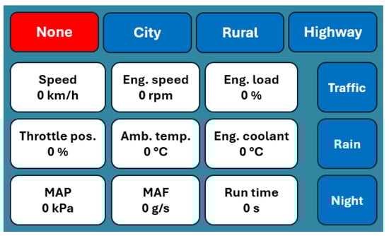
Figure 1.
Data logger’s user interface.
Figure 1 shows the initialized state after the ignition is switched on. The states shown in the top row are exclusive; the current state is saved in each cycle. The 3 × 3 white boxes only provide information to ensure the data logging works properly. The three blue boxes on the bottom right can be used to indicate in binary whether any traffic or environmental conditions influence driving. When a status is active, the box turns red.
The Electronic Control Units (ECUs) do not work when the ignition is off, so they do not respond to diagnostic requests. This makes it easy to implement separation to ensure that a measurement file lasts from when the ignition is on to when the ignition is off. These measurement files can be interpreted as tables with 13 columns. These columns are as follows in addition to the nine OBD-II parameters shown in Table 2:
- Road type: none, city, rural, or highway coded as integer from 0 to 3, respectively.
- Traffic: binary, indicates slow driving sections, for example, traffic jam on a highway.
- Rain: binary, indicates slow driving sections due to precipitation.
- Night: binary, indicates slow driving sections due to limited visibility.
Any hardware capable of CAN communication is suitable for recording OBD-II parameters, but a touchscreen is required to record the road type. Our chosen configuration consists of the following parts: Arduino Giga R1 Wifi, Seeed studio’s CAN-BUS Shield v2, and Arduino Giga display shield.
2.2. Logging Results
Figure 2 shows the typical pattern of a countryside trip in Hungary. Red, blue, and green backgrounds represent city, rural, and highway sections, respectively. In the speed profile, it can be seen that around minute 60, the speed on the highway drops below 50 km/h, which makes classification difficult. Furthermore, speeds are lower in rural areas after the highway than in the last city section. MAP is not included in the figures because a vehicle usually has either MAP or MAF only, and ambient temperature is not included because it does not contain relevant information in this phase.
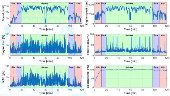
Figure 2.
A sample of the measurements.
During the data logging process, the driver’s attention is critical, as the road types he selects are accepted as ground truth. For this reason, only two data loggers were made and placed in our cars. The measurement period was in 2024, from the beginning of June to the beginning of October. The driving data include everything from daily commuting to work to family holidays. The results are summarized in Table 3.
Table 3.
Summary of the four-month measurement.
3. Methods
The measured parameters presented in Table 2 were used to develop the methods. Engine speed and load, accelerator pedal position, MAP, and MAF are engine-dependent values. Therefore, these cannot be used for universal vehicle-independent evaluation. Ambient temperature, engine coolant temperature, and run time do not provide relevant information for road type classification. Therefore, only the vehicle speed and the labels were used in the methods from the recorded driving cycles presented in Table 3.
3.1. Data Cleaning
The following methods operate only with speed points and do not obtain the corresponding time as input. However, the speed points in the measurement files are not equidistant in time. This is possible for two reasons: either the ECU or the CAN bus was busy during the data request, and the diagnostics only had a secondary priority in the vehicle’s operation. The average distance between speed points is 0.1725 s, with a standard deviation of 0.0443. The simplest method to make the data points uniformly spaced is interpolation. Based on experience, an interpolation interval of 1 s was chosen.
Labels are attached to each speed point, indicating where the driving occurred. Labels can have the following values:
- 0: Undefined (initial state; indicates special cases)
- 1: City
- 2: Rural
- 3: Highway
Labels were interpolated with the speed, and the obtained values were rounded to integer values.
3.2. Conventional Method
From the state-of-the-art methods mentioned in Section Literature Review, only [32,34] can be applied to speed data using the same methodology. However, these studies focus on driving style analysis rather than accurate road type classification, so the methods are not described in detail.
The method consists of 2 phases: the first is the classification, and in the second, the segments that are shorter than a given threshold are combined with their neighbors. The first phase is shown in Algorithm 1. Denote D as the set of the measured driving cycles, where each drive cycle consists of a speed vector and a label vector According to the original method, the driving cycles are split into 40 s segments; let this set be S. In our version, S contains the last segments of the driving cycles, which are shorter than 40 s. The segments of the set S where the speed was zero were deleted, resulting in the set S’.
For each element of the set S’, the maximum speed (M), average non-idle speed (N), average speed gradient (G), and modus of label vector (L) are calculated. In the original method, speed time residencies were used instead of the average speed gradient, but how to determine this value was not defined. The first three metrics (M, N, G) are of different orders of magnitude and contribute differently to the determination of the class. Therefore, weighting should be applied. The values of the weights were determined by optimization, where the sum of the difference between the weighted sum of the metrics and the modus of the labels was minimized. Then, classes were calculated based on the weighted sum of the metrics.
| Algorithm 1. The algorithm of the first phase of the conventional method | |
| 1: | D: set of the measured driving cycles splitting_time = 40 s |
| 2: | S ← Split the elements of D into segments of length splitting_time |
| 3: | S’← Delete the whole zero speed elements of S’ |
| 4: | M ← Maximum speed for each element of S’ |
| 5: | N ← Average non-idle speed for each element of S’ |
| 6: | G ← Average speed gradient for each element of S’ |
| 7: | L ← Modus of the labels for each element of S’ |
| 8: | |
| 9: | C ← Calculate the classes |
In the second phase, the original thresholds have been applied; namely, the city consists of at least 1 segment, the rural area has at least 2, and the highway has at least 4. From the start of the driving cycle, the conditions were checked, and if they were not satisfied, the class was overwritten based on the previous segment. This operation aims to filter out misclassification due to temporary high/low speeds.
Two more methods were used as post-processing. The nearest local minimum was searched in the 20 s environment for class transitions, and the transition was shifted there. Finally, the class of sections with only zero speeds was set to the same as the class before it.
3.3. Proposed Method
The proposed method uses neural networks, which require data preprocessing. This method takes the cleaned, interpolated data presented in Section 3.1 as input. ANNs have a fixed input size; however, the driving cycles have different cycle lengths. Also, the output of the ANN is fixed, but a driving cycle can have several road types, which would mean more outputs.
3.3.1. Data Preprocessing
The driving cycles have been split into independent fixed-length subcycles to handle different cycle lengths. To determine this length, we examined the distribution of cycle durations shown in Figure 3. It can be seen that most of the drives (52) were between 9 and 10 min in duration, and the minimum duration was 3 min. Choosing too high length will lead to shorter cycles being omitted from the training, resulting in data loss. Too short durations can lead to misclassification in the case of slower driving. As an intermediate option, a 180 s splitting time was chosen.
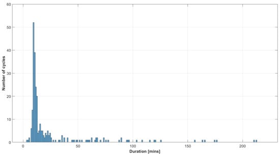
Figure 3.
The distribution of the duration of driving cycles.
When splitting driving cycles into fixed-length subcycles, a subcycle may have more than one road type. To handle this, the target variable for the subcycle has been modified to the modus of the road types it contains.
With the splitting method, the original 266 cycles were divided into 2249 subcycles, with the ratio of road types shown in Table 4. Imbalanced data can bias models and result in poor predictive performance for the minority classes. One of the most popular approaches is using resampling techniques. Undersampling was used, reducing the number of samples in the majority classes to bring the dataset into balance. In this case, 527 subcycles from each class were selected randomly, so the reduced dataset consists of 1581 elements.
Table 4.
The ratio of road types after subcycle splitting.
Min-max normalization was used to map the speed values to the range [−1, 1], which can help speed up learning and improve the initial solution [41]. Another technical method was to one-hot encode the target variable. This means that the expected output is a 3-element vector instead of the numbers 1, 2, or 3, where the 3 elements represent the probability of the 3 classes. This can be useful for analyzing misclassifications later in the process.
3.3.2. Neural Networks
As can be seen in the literature, recent methods for the road type classification problem use artificial neural networks. The advantage of ANN is seen in such situations where it can be used instead of building a complex rule set.
The fixed-size, interpolated speed inputs produced by the previous preprocessing method are time-dependent data series. However, the time-dependent property of velocity yields the acceleration, which is not necessary for classification. To solve the problem, it is only required to know the speed values since the distribution of these values determines the road type. Furthermore, acceleration can indirectly negatively affect the results, as there can be significant differences in acceleration between different vehicle categories or driving styles. For these reasons, the problem can be solved with the simplest sequential network and feedforward neural network and does not require recurrent neural networks. A precise formulation of the problem helps to handle the many parameters to be chosen.
Due to the 1 s interpolation and the 180 s splitting time, the dimension of the neural network input is 180. Similarly, the output dimension is three because of the one-hot encoding. Several structures have been tested on hidden neurons whose number can be chosen arbitrarily. The large number of inputs compared to the small number of outputs is similar to the encoder half of an encoder–decoder neural network. Therefore, the interval [180, 3] should be divided into evenly spaced values. For the number of hidden layers, the best solution was 5. So, the number of neurons in the layers of the neural network was chosen as 180, 150, 121, 92, 62, 32, and 3. This resulted in a total of 64.526 trainable parameters. Sigmoid was used in the hidden neurons, and softmax was used in the output layer for activation functions.
The evaluation metrics are used to identify the effectiveness and performance of a model. In the case of classification problems, this is typically the accuracy, which is defined as the ratio of the correct predictions divided by the total number of predictions. Loss functions are used to determine the error between the prediction and the target value, and the goal of the training is to minimize this error. The preferred loss function is the categorical cross-entropy, as this, combined with the softmax function, assigns a probability to each class, which can be used for further analysis. There is no significant difference between the optimization algorithms, so adam was chosen as one of the most efficient methods. The most frequently used values from the literature and practice were selected for batch size and train–validation ratio, 5 and 80–20%, respectively. The learning duration, i.e., the epoch number, was determined based on Figure 4. The runs were performed with the following model settings:
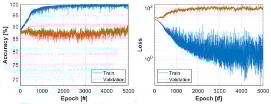
Figure 4.
The result of the test run.
- Metric: accuracy
- Loss: categorical cross-entropy
- Optimizer: adam
- Epoch number: 5000
- Batch size: 5
- Train–Validation ratio: 80–20%
Moreover, as a callback option, the minimum loss on the training set has been set as a checkpoint. This means that the weight matrix is saved if the loss during training is lower than in the previous iterations. After training, the neural network corresponding to the lowest loss can be restored for evaluation. Training loss is preferred over validation loss due to the small size of the validation set.
Figure 4 shows the result of a test run. On the training set, 100% accuracy was already achieved in epoch 3078 with a validation accuracy of 84.15%. The lowest training loss was achieved in epoch 4864, where the training accuracy is 100% and the validation accuracy is 85.57%.
4. Results
The road type classification problem can be solved with the neural network presented in Section 3.3.2 to a certain accuracy. However, there are other techniques to improve the performance of neural networks beyond the network structure and settings. This section presents some of these, which can be used to achieve better results on the road type classification problem, and shows the results compared to the conventional method. All the following ANN models were run with the settings detailed in Section 3.3.2.
4.1. Conventional Method
The conventional method presented in Section 3.2 gives an accuracy of 83% using the full dataset presented in Section 3.1 with 40 s segments. However, studies [32,34] do not explain the choice of this 40 s splitting time.
The splitting time was tested from 1 s to 360 s. In Figure 5, two sections can be identified: before and after 140 s. In the first case, it can be seen that the accuracy is highly dependent on the choice of splitting time, e.g., for 67 sec, the accuracy is 85.6%, while for 68 sec, it is only 72.5%. This may be because the label and class transitions are close in high precision splitting time. In the case of lower precision, the optimizer found only a local minimum for the weights. However, above 140 s, the minimum accuracy is 86.5%, and the maximum is 89.9% at 336 s. In this case, the segments are long enough to calculate a consistent average speed, which is less affected by a single outlier.
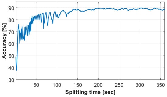
Figure 5.
The result of the conventional method.
4.2. Base NN Model
The base NN model is the same as the model mentioned in Section 3.3.2. Several random variables exist in the training process, from weight initialization to shuffling of training batches per iteration. Therefore, three runs have been performed for each model to provide consistent and comparable results.
Table 5 shows the results of the model. It can be seen that results similar to those of the test run were obtained on the reduced dataset. Furthermore, an average accuracy of 93.25% was achieved on the full dataset. Since the model has to work on imbalanced data, the most relevant metric is evaluation accuracy; thus, run 2 gives the best result with 93.62%, which is more than 3.5% higher than the maximum accuracy of the conventional method.
Table 5.
The results of the base NN model.
4.3. Cross-Validation
Random undersampling due to imbalanced data, random train–validation splitting, and the small number of samples in the reduced dataset may have resulted in special cases being excluded from the training and misclassified during the evaluation. However, if all the data are included in the training, there is no previously unseen data on which the model’s performance can be validated. To solve this problem, k-fold cross-validation has been used, which is mainly used to estimate or compare model performances.
In this case, a special version of k-fold cross-validation, stratified k-fold cross-validation, has been used as a resampling technique. The reduced dataset has been split into k folds of equal size while preserving the balanced class distribution in each fold. The model is trained on k-1 folds and validated on the holdout set. This process is repeated until all folds are the validating fold once. A total of k different models have been trained, and performance metrics such as accuracy and loss can be calculated from the average of these results. Afterward, a final model has to be trained with the same settings on the full reduced dataset without a validation set.
The results of the cross-validation method (Table 6) show that the average results for the reduced dataset are slightly worse compared to the base model (Table 5). However, the results improved by an average of 2.52% on the full dataset, and the best result (run 1) also increased by 2.33%.
Table 6.
The results of the cross-validation model.
4.4. Weighted Loss Function
The built-in categorical cross-entropy calculates the loss based on how far the prediction is from the ground truth but does not differentiate between misclassifications. For example, predicting city driving as highway driving is a minor problem since a speed profile similar to city driving can occur in heavy traffic on a highway. However, classifying high-speed highway driving as city driving is a significant problem because such high speeds cannot occur in cities. This problem can be solved by weighting the misclassifications.
On the full dataset, the highest accuracy was achieved by base model run 2, whose confusion matrix is shown in Table 7, with the number of samples in the cells above and the percentage below. The elements in the main diagonal are the correct predictions, whose sum is 93.62%, which is the evaluation accuracy shown in Table 4. Let the elements below the main diagonal of the confusion matrix be Type I misclassification and the elements above the main diagonal be Type II misclassification. Type I misclassification is worse for the reasons mentioned above. It can be seen that the Type II misclassification rate is higher than Type I due to many instances of rural driving being predicated as city driving.
Table 7.
Confusion matrix of the base model run 2.
The confusion matrix for the highest accuracy of the conventional method is shown in Table 8. The numbers of classified cycles are different in Table 7 and Table 8, as the splitting time for the base model was 180 s, while for the conventional method, it was 336 s. Due to the lower accuracy of the conventional method, the number of misclassifications is higher. Type I error is 4.98% and Type II error 4.81% compared to the base model results of 1.8% and 4.58%, respectively.
Table 8.
Confusion matrix of the conventional method with the highest accuracy.
The loss function should be weighted according to the ground truth and the corresponding prediction, so the size of the weight matrix will be 3-by-3. Higher weights should only be used for Type I misclassification since the loss function penalizes Type II errors by default. Finding the optimal weights for the problem is not trivial since, for too-small weights, the method is identical to the unweighted case. In contrast, the number of Type II misclassifications increases for too-large weights. Furthermore, highway driving predicted as city driving is worse than the other two Type I errors. After several attempts, the weight matrix shown in Table 9 was applied.
Table 9.
Weight matrix for the loss function.
As Table 10 shows, the results are similar to the base model for the reduced dataset with weighting, but the average accuracy on the full dataset is decreased by nearly half a percent. For the best runs, the accuracy is reduced by only 0.3% with the weighting method.
Table 10.
The results of the weighted loss function model.
However, examining the confusion matrix (Table 11), it can be seen that the Type I error of 1.8% has been reduced to 1.14% with a marginal decrease in the evaluation accuracy.
Table 11.
Confusion matrix of the weighted loss function model run 3.
4.5. Cross-Validation and Weighted Loss Function
As the previous results show, weighting can be used to reduce Type I misclassifications, but it also reduces the evaluation accuracy. However, cross-validation can also improve accuracy. Therefore, it was obvious that the two methods should be combined.
The results of the weighted cross-validation (Table 12) show that the evaluation accuracy increased by more than 2.5% on the full dataset compared to the baseline model. Moreover, both the average and the best results improved compared to cross-validation.
Table 12.
The results of the weighted cross-validation model.
Type I error was reduced to less than 1% for run 1 (Table 13). It is also remarkable that the Type II error rate has been almost halved compared to the previous results. Due to these two factors, the evaluation accuracy for this run was 96.21%, the highest of all the runs.
Table 13.
Confusion matrix of the weighted cross-validation model Run 1.
5. Discussion
The major advantage of the conventional and proposed method is that only the speed is used to classify the road type. The data presented in Chapter 2 can be used to determine the model parameters, but it is not necessary to record labeled data after the validation. Therefore, future data can be recorded similarly from CAN, but speed points can also be recorded by phone or GPS.
The conventional method uses the three most relevant metrics for a driving cycle. Different road types have different speed limits, so the maximum speed is essential. However, there can be a higher acceleration in a cycle. Therefore, the average speed should also be used, corrected by non-idle speeds. An average speed can be achieved at a constant speed or oscillating around the average; hence, the average speed gradient must also be an input. The method uses three values as the input, so it is easy to apply to different splitting times.
The number of inputs of neural networks changes for different splitting times (for constant interpolation time), so, in this case, new training must be performed, which is time-consuming. However, the trained model classifies quickly. The advantage of neural networks is that they do not require cycle-specific metrics, operating only with speed points. The base NN model achieved higher accuracy than the conventional method, which was improved further with different techniques. Moreover, the weighted loss function can control the proportion of different misclassification types.
The method uses stratified folding instead of stratified group folding, which would be preferable. In group folding, all cycles of full drives can be assigned only to the training set or only to the validation set, while in the basic version, there is no such restriction. The use of this method is limited by the dataset. The train–validation ratio of 80–20% was chosen, but maintaining this ratio and the group restriction resulted in a lot of data loss. An additional challenge is to ensure that the city, rural, and highway classes are balanced in the training and validation sets, as highway sections usually occur in longer drives.
Our future aim is to develop the conventional and proposed methods further. For the conventional method, we aim to search for additional metrics that provide relevant information about the cycle. In the case of the proposed method, class merging can further improve accuracy. Currently, the neural network makes the decision based on speed only, but this can be extended by adding more logged parameters. Moreover, the methodology can be extended by finding the exact start and end of the road type after classification, for example, by finding local minima and maxima in the speed profile within a time window. The current methodology uses a reduced dataset in which classes are balanced. Our future goal is to introduce balancing techniques to use as much labeled data as possible in the learning process. Furthermore, to extend the method to different network types, it is necessary to perform an extensive hyperparameter analysis.
6. Conclusions
This study examines the classification problem of road types based on speed profiles. The aim was to identify city, rural, and highway driving based on real measurements. Special data recording devices were used for the methods shown in the literature, which were unsuitable for widespread application.
An OBD logging device was developed that works on all internal combustion engines or hybrid vehicles and can be used to record labeled data to measure the accuracy of the methods. The device can later operate independently of the driver without the labeling function.
One state-of-the-art method was found that can classify road types only by speed. Based on this study, this method has been implemented as accurately as possible. Furthermore, by testing the parameter values used in the process, further improvements were achieved on our own dataset. The highest accuracy achieved by the conventional method is 89.9%, and the corresponding Type I error is 4.9%. The accuracy of the base version of our neural network-based method is 93.6%, with 1.8% Type I error on the same dataset.
There are special traffic situations in the measured data, i.e., a traffic jam on a highway, which reduces the accuracy of the method if present only in the validation set. Therefore, it is necessary to involve as much data as possible in the training phase. To overcome this, k-fold cross-validation was used, which improved the accuracy to 95.9%. Misclassifications are not equivalent due to the nature of the problem, as slower driving can occur in a faster environment, but the reverse is not valid. The type of misclassifications can be handled by weighting the loss function. By setting the optimal weighting matrix, this technique reduced the Type I error to 1.14%, but the accuracy was reduced to 93.3%. Combining the two methods, the neural network-based method achieved 96% accuracy and Type I error below 1%.
Author Contributions
Conceptualization, D.T. and M.Z.; methodology, D.T. and M.Z.; software, D.T.; validation, D.T. and M.Z.; writing—original draft preparation, D.T.; writing—review and editing, D.T. and M.Z.; visualization, D.T.; supervision, M.Z. All authors have read and agreed to the published version of the manuscript.
Funding
Project no. 2020-2.1.1-ED-2020-00062 was implemented with the support provided by the Ministry of Culture and Innovation of Hungary from the National Research, Development and Innovation Fund.
Data Availability Statement
The data presented in this study are available on request from the corresponding author.
Conflicts of Interest
Dávid Tollner is employed by Robert Bosch Kft. The funders had no role in the design of the study; in the collection, analyses, or interpretation of data; in the writing of the manuscript; or in the decision to publish the results.
Abbreviations
The following abbreviations are used in this manuscript:
| ADAS | Advanced Driver-Assistance System |
| ELKS | Emergency Lane Keeping Systems |
| MCU | Motor Control Unit |
| EV | Electric Vehicle |
| ANN | Artificial Neural Network |
| CAN | Controller Area Network |
| k-NN | k-Nearest Neighbor |
| SVM | Support Vector Machine |
| CNN | Convolutional Neural Network |
| GMM | Gaussian Mixture Model |
| OBD | On-board Diagnosis |
| GBM | Gradient Boosting Machine |
| ICE | Internal Combustion Engine |
| AI | Artificial Intelligence |
| ECU | Electronic Control Unit |
| MAP | Mass Air Pressure |
| MAF | Mass Air Flow |
References
- Boltachev, E. Potential cyber threats of adversarial attacks on autonomous driving models. J. Comput. Virol. Hacking Tech. 2024, 20, 363–373. [Google Scholar] [CrossRef]
- Council Regulation (EC). Commission Implementing Regulation (EU) 2021/646 of 19 April 2021 laying down rules for the application of Regulation (EU) 2019/2144 of the European Parliament and of the Council as regards uniform procedures and technical specifications for the type-approval of motor vehicles with regard to their emergency lane-keeping systems (ELKS). Off. J. Eur. Union 2021, 64, 31–54. [Google Scholar]
- Zöldy, M.; Baranyi, P.; Török, Á. Trends in Cognitive Mobility in 2022. Acta Polytech. Hung. 2024, 21, 189–202. [Google Scholar] [CrossRef]
- Doniec, R.; Piaseczna, N.; Li, F.; Duraj, K.; Pour, H.H.; Grzegorzek, M.; Mocny-Pachońska, K.; Tkacz, E. Classification of Roads and Types of Public Roads Using EOG Smart Glasses and an Algorithm Based on Machine Learning While Driving a Car. Electronics 2022, 11, 2960. [Google Scholar] [CrossRef]
- Hanine, M.; Boutkhoum, O.; El Barakaz, F.; Lachgar, M.; Assad, N.; Rustam, F.; Ashraf, I. An Intuitionistic Fuzzy Approach for Smart City Development Evaluation for Developing Countries: Moroccan Context. Mathematics 2021, 9, 2668. [Google Scholar] [CrossRef]
- Horvath, P.; Nyerges, A. Design aspects for in-vehicle IPM motors for sustainable mobility. Cogn. Sustain. 2022, 1, 1–14. [Google Scholar] [CrossRef]
- Li, Y.; Zhao, W.; Fan, H. A Spatio-Temporal Graph Neural Network Approach for Traffic Flow Prediction. Mathematics 2022, 10, 1754. [Google Scholar] [CrossRef]
- Apanaviciene, R.; Vanagas, A.; Fokaides, P.A. Smart Building Integration into a Smart City (SBISC): Development of a New Evaluation Framework. Energies 2020, 13, 2190. [Google Scholar] [CrossRef]
- Jneid, M.S.; Harth, P. Radial Flux In-Wheel-Motors for Vehicle Electrification. Cogn. Sustain. 2024, 3, 16–33. [Google Scholar] [CrossRef]
- Ruggieri, R.; Ruggeri, M.; Vinci, G.; Poponi, S. Electric Mobility in a Smart City: European Overview. Energies 2021, 14, 315. [Google Scholar] [CrossRef]
- Salmeron-Manzano, E.; Manzano-Agugliaro, F. The Electric Bicycle: Worldwide Research Trends. Energies 2018, 11, 1894. [Google Scholar] [CrossRef]
- Lim, H.S.M.; Taeihagh, A. Autonomous Vehicles for Smart and Sustainable Cities: An In-Depth Exploration of Privacy and Cybersecurity Implications. Energies 2018, 11, 1062. [Google Scholar] [CrossRef]
- Bianchi, D.; Epicoco, N.; Di Ferdinando, M.; Di Gennaro, S.; Pepe, P. Physics-Informed Neural Networks for Unmanned Aerial Vehicle System Estimation. Drones 2024, 8, 716. [Google Scholar] [CrossRef]
- Ficzere, P. The role of artificial intelligence in the development of rail transport. Cogn. Sustain. 2023, 2, 1–5. [Google Scholar] [CrossRef]
- Pleshakova, E.; Osipov, A.; Gataullin, S.; Gataullin, T.; Vasilakos, A. Next gen cybersecurity paradigm towards artificial general intelligence: Russian market challenges and future global technological trends. J. Comput. Virol. Hacking Tech. 2024, 20, 429–440. [Google Scholar] [CrossRef]
- Jansen, P.; van der Mark, W.; van den Heuvel, J.C.; Groen, F.C.A. Colour based off-road environment and terrain type classification. In Proceedings of the 8th International IEEE Conference on Intelligent Transportation Systems, Vienna, Austria, 13–16 September 2005; pp. 216–221. [Google Scholar]
- Rahi, A.; Elgeoushy, O.; Syed, S.H.; El-Mounayri, H.; Wasfy, H.; Wasfy, T.; Anwar, S. Deep Semantic Segmentation for Identifying Traversable Terrain in Off-Road Autonomous Driving. IEEE Access 2024, 12, 162977–162989. [Google Scholar] [CrossRef]
- Shon, H.; Choi, S.; Huh, K. Real-Time Terrain Condition Detection for Off-Road Driving Based on Transformer. IEEE Trans. Intell. Transp. Syst. 2024, 25, 11726–11738. [Google Scholar] [CrossRef]
- Paraphantakul, C. Review of Worldwide Road Classification Systems. In Proceedings of the 9th National Transportation Conference, Bangkok, Thailand, 20–21 November 2014. [Google Scholar]
- Tang, I.; Breckon, T.P. Automatic Road Environment Classification. IEEE Trans. Intell. Transp. Syst. 2011, 12, 476–484. [Google Scholar] [CrossRef]
- Slavkovikj, V.; Verstockt, S.; De Neve, W.; Van Hoecke, S.; Van De Walle, R. Image-Based Road Type Classification. In Proceedings of the 22nd International Conference on Pattern Recognition, Stockholm, Sweden, 24–28 August 2014; pp. 2359–2364. [Google Scholar] [CrossRef]
- Seeger, C.; Müller, A.; Schwarz, L.; Manz, M. Towards Road Type Classification with Occupancy Grids. In Proceedings of the IEEE Intelligent Vehicles Symposium 2016 Workshop: DeepDriving—Learning Representations for Intelligent Vehicles, Gothenburg, Sweden, 19–22 June 2016. [Google Scholar]
- Krizhevsky, A.; Sutskever, I.; Hinton, G.E. Imagenet classification with deep convolutional neural networks. In Proceedings of the Advances in Neural Information Processing Systems, Lake Tahoe, NV, USA, 3–6 December 2012. NIPS 25. [Google Scholar]
- Simonyan, K.; Zisserman, A. Very deep convolutional networks for large-scale image recognition. In Proceedings of the 3rd International Conference on Learning Representations, San Diego, CA, USA, 7–9 May 2015. ICLR 2015. [Google Scholar]
- Szegedy, C.; Liu, W.; Jia, Y.; Sermanet, P.; Reed, S.; Anguelov, D.; Erhan, D.; Vanhoucke, V.; Rabinovich, A. Going deeper with convolutions. In Proceedings of the IEEE Conference on Computer Vision and Pattern Recognition, Boston, MA, USA, 7–12 June 2015. CVPR 2015. [Google Scholar]
- Saleh, Y.; Otoum, N. Road-Type Classification through Deep Learning Networks Fine-Tuning. J. Inf. Knowl. Manag. 2020, 19, 2040020. [Google Scholar] [CrossRef]
- Mohammad, M.A.; Kaloskampis, I.; Hicks, Y. Evolving GMMs for road-type classification. In Proceedings of the IEEE International Conference on Industrial Technology (ICIT), Seville, Spain, 17–19 March 2015; pp. 1670–1673. [Google Scholar] [CrossRef]
- Brostow, G.J.; Fauqueur, J.; Cipolla, R. Semantic object classes in video: A high-definition ground truth database. Pattern Recognit. Lett. 2009, 30, 88–97. [Google Scholar] [CrossRef]
- Zheng, Q.; Tian, X.; Yang, M.; Su, H. CLMIP: Cross-layer manifold invariance based pruning method of deep convolutional neural network for real-time road type recognition. Multidimens. Syst. Signal Process. 2021, 32, 239–262. [Google Scholar] [CrossRef]
- Murphey, Y.L.; Chen, Z.; Kiliaris, L.; Park, J.; Kuang, M.; Masrur, A.; Phillips, A. Neural learning of driving environment prediction for vehicle power management. In Proceedings of the 2008 IEEE International Joint Conference on Neural Networks (IEEE World Congress on Computational Intelligence), Hong Kong, China, 1–8 June 2008; pp. 3755–3761. [Google Scholar] [CrossRef]
- Carlson, T.R.; Austin, R.C. Development of Speed Correction Cycles; Report SR97-04-01; U.S. Environmental Protection Agency: Washington, DC, USA, 1997. [Google Scholar]
- Daniel, R.; Brooks, T.; Pates, D. Analysis of US and EU Drive Styles to Improve Understanding of Market Usage and the Effects on OBD Monitor IUMPR; SAE Technical Papers; SAE International: Warrendale, PA, USA, 2009; p. 2009-01-0236. [Google Scholar] [CrossRef]
- Taylor, P.; Anand, S.S.; Griffiths, N.; Adamu-Fika, F.; Dunoyer, A.; Popham, T. Road Type Classification through Data Mining. In Proceedings of the 4th International Conference on Automotive User Interfaces and Interactive Vehicular Applications, New York, NY, USA, 17–19 October 2012; AutomotiveUI ’12. pp. 233–240. [Google Scholar] [CrossRef]
- Lee, C.; Öberg, P. Classification of Road Type and Driving Style Using OBD Data; SAE Technical Papers; SAE International: Warrendale, PA, USA, 2015; p. 2015-01-0979. [Google Scholar] [CrossRef]
- Hadrian, A.; Vainshtein, R.; Shapira, B.; Rokach, L. DeepCAN: Hybrid Method for Road Type Classification Using Vehicle Sensor Data for Smart Autonomous Mobility. IEEE Trans. Intell. Transp. Syst. 2023, 24, 11756–11772. [Google Scholar] [CrossRef]
- Hungarian Central Statistical Office. 24.1.1.25. Passenger Car Fleet by Make and Fuel Consumption. Available online: https://www.ksh.hu/stadat_files/sza/en/sza0025.html (accessed on 2 December 2024).
- ISO 15031-5; Road Vehicles—Communication Between Vehicle and External Equipment for Emissions-Related Diagnostics—Part 5: Emissions-Related Diagnostic Services. International Organization for Standardization: Geneva, Switzerland, 2006.
- Council Directive (EC). DIRECTIVE 98/69/EC OF THE EUROPEAN PARLIAMENT AND OF THE COUNCIL of 13 October 1998 relating to measures to be taken against air pollution by emissions from motor vehicles and amending Council Directive 70/220/EEC. Off. J. Eur. Communities 1998, 23, 126–181. [Google Scholar]
- Tollner, D.; Zöldy, M. Investigating the Energetics of Electric Vehicles, based on Real Measurements. Acta Polytech. Hung. 2024, 21, 235–252. [Google Scholar] [CrossRef]
- Tollner, D.; Nyerges, Á.; Jneid, M.S.; Geleta, A.; Zöldy, M. How Do We Calibrate a Battery Electric Vehicle Model Based on Controller Area Network Bus Data? Sensors 2024, 24, 4637. [Google Scholar] [CrossRef] [PubMed]
- Han, J.; Kamber, M.; Pei, J. 3.3 Data integration and transformation. In Data Mining: Concepts and Techniques; Morgan Kaufmann Publishers Inc.: San Francisco, CA, USA, 2006; pp. 8–10. [Google Scholar]
Disclaimer/Publisher’s Note: The statements, opinions and data contained in all publications are solely those of the individual author(s) and contributor(s) and not of MDPI and/or the editor(s). MDPI and/or the editor(s) disclaim responsibility for any injury to people or property resulting from any ideas, methods, instructions or products referred to in the content. |
© 2025 by the authors. Licensee MDPI, Basel, Switzerland. This article is an open access article distributed under the terms and conditions of the Creative Commons Attribution (CC BY) license (https://creativecommons.org/licenses/by/4.0/).