Abstract
In this paper, we describe the associative and commutative algebra or the (2,2)-model of quaternions with application in color image enhancement. The method of alpha-rooting, which is based on the 2D quaternion discrete Fourier transform (QDFT) is considered. In the (2,2)-model, the aperiodic convolution of quaternion signals can be calculated by the product of their QDFTs. The concept of linear convolution is simple, that is, it is unique, and the reduction of this operation to the multiplication in the frequency domain makes this model very attractive for processing color images. Note that in the traditional quaternion algebra, which is not commutative, the convolution can be chosen in many different ways, and the number of possible QDFTs is infinite. And most importantly, the main property of the traditional Fourier transform that states that the aperiodic convolution is the product of the transform in the frequency domain is not valid. We describe the main property of the (2,2)-model of quaternions, the quaternion exponential functions and convolution. Three methods of alpha-rooting based on the 2D QDFT are presented, and illustrative examples on color image enhancement are given. The image enhancement measures to estimate the quality of the color images are described. Examples of the alpha-rooting enhancement on different color images are given and analyzed with the known histogram equalization and Retinex algorithms. Our experimental results show that the alpha-rooting method in the quaternion space is one of the most effective methods of color image enhancement. Quaternions allow all colors in each pixel to be processed as a whole, rather than individually as is done in traditional processing methods.
1. Introduction
In recent years, many articles have been published on color image processing, wherein image enhancement plays an important role. Many color images are low quality and require enhancement as the first stage of processing. [1,2,3,4,5]. Examples of such images can be found among underwater images, thermal images, and medical images. Decades ago, we divided methods of image enhancement into two classes, namely spatial and traditional, or complex, frequency domains; now, a new class has been added to them. Here, we mention methods of image enhancement in the quaternion algebras. Color and grayscale images can be processed in the quaternion space with good results not only in image enhancement but in filtration, face recognition, neural networks, and other applications. The first class of methods includes contrast stretching techniques and logarithmic models [4] and the very effective and simple histogram equalization with its different modifications [6,7,8,9,10]. The Retinex algorithm can also be classified into this class [11,12]. In the second class, we should note the Fourier transform-based alpha-rooting [13], which is the most effective method for enhancing grayscale and color images. The advantage of enhancing color images in the quaternion space is in the fact that the primary colors plus the gray are processed as one unit, not separately. Therefore, quaternion image processing does not introduce false color artifacts [14].
In this paper, we focus on the commutative quaternion algebra, or the (2,2)-model. In this model, the concepts of the 1D and 2D QDFT are considered, and their properties are described. This model of quaternion uses the color image enhancement alpha-rooting by the 2D QDFT. A comparison with the traditional quaternion algebra is also given.
The main contributions of this work are the following:
- The separable alpha-rooting method of color image enhancement;
- New two-parameter alpha-rooting methods of color image enhancement;
- The effectiveness of using the 2D QDFT-based alpha-rooting in the (2,2)-model;
- Illustrative examples showing the effectiveness of using the (2,2)-model in color image enhancement.
The rest of the paper is organized in the following way. Section 2 describes two models of quaternions, namely the (2,2)- and (1,3)-models. The first model is commutative, and the second one is not. Section 3 describes the exponential functions of the (2,2)-model. The concepts of the QDFTs are considered in Section 4 for both models. The methods of alpha-rooting in these models are described in Section 5. The comparison of the 2D QDFT-based alpha-rooting methods in the (2,2)- and (1,3)-models are given. Results and illustrative examples of color images are presented in Section 6.
2. Quaternion Numbers: Two Arithmetics
In this section, we describe quaternion numbers in two algebras, non-commutative and commutative. The concept of the quaternion, or quadruple of numbers as a vector in the 4-dimensional (4D) space was introduced by Gauss in 1819 [15]. As complex numbers, quaternions have one real part and one imaginary part. Only the imaginary part presents a triplet of numbers or a 3D vector. Therefore, quaternions can be considered as an extension of complex numbers [16,17,18]. It is not possible for us to draw quaternions in 4D space, but we will show how such numbers can be embedded in geometric figures in 3D space. There are different types of arithmetic of quadruples of numbers, or quaternions, because they define the main operation—multiplication—differently. We consider two arithmetics, or models, in which the operation of multiplication is commutative and non-commutative. The second arithmetic attracted much attention from researchers in the field of signal and image processing. However, the fact that the multiplication of quaternions is a non-commutative operation leads to large uncertainties in such important operations as the convolution, correlation, and Fourier transform, especially in processing color images. Therefore, we think it is necessary to pay more attention to the commutative operation of the multiplication of quaternions and the corresponding arithmetic, or the commutative algebra of quaternions.
2.1. The (1,3)-Model of Quaternions
Consider three units , and with the following multiplication laws:
A quaternion is defined as the number with real numbers , and . The number is the imaginary part of the quaternion and can be considered as the vector in the 3D space. Therefore, we can write This model of representation of quaternions as is called the (1,3)-model [14]. A quaternion has one real part, , and the three-component imaginary part, . If the imaginary part , then the quaternion is called a pure quaternion number. If , the quaternion is a complex number. Similar to the complex numbers, the conjugate of the quaternion is defined as , or .
The multiplication of two quaternions and is defined according to the laws in Equation (1). Thus, the quaternion is calculated by
It is important to note, that the number is real and non-negative, ; it is denoted by . The number is called the length of the quaternion.
The sum of quaternions is calculated component-wise, . In the multiplication of imaginary units, , and . The multiplication in the (1,3)-model is not commutative. That is, for different and the product or .
Considering the quaternions and as the 4D vectors, and , the above operation of multiplication can be written in the matrix form as follows:
The determinant of the matrix equals . For the case when , the matrix is unitary and its determinant The coefficients of this matrix are components of the quaternion . The first column of the matrix is the quaternion . A similar matrix of multiplication can be defined by the components of the quaternion (for details, see [14]).
Unlike traditional arithmetic, where the exponential function is defined uniquely, in the (1,3)-model, the number of such functions is infinite. Given a pure unit quaternion , , the quaternion exponential function at the angle is defined as . In the next sections, we will discuss the concept of the quaternion discrete Fourier transforms, which are different analogues of the traditional DFT. This transform is defined by the system of basis functions, which are calculated by the single complex exponential function . In the (1,3)-model, we are faced with the problem of which exponential function to use as the base function for the QDFT. In other words, if in the traditional representation each signal or image has the unique representation in the frequency domain, in the (1,3)-model, there are an infinite number of such representations. How to choose, namely which quaternion number is best for the QDFT, is unknown today. And it is this model that has been widely used in the last two decades in many applications in signal and image processing [14,19,20,21].
2.2. The (2,2)-Model of Quaternions
In this section, we consider the arithmetic of quaternions with the associative and commutative operation of multiplication introduced by Grigoryan in 2022 [22]. This is the so-called (2,2)-model of representation of quaternions.
In the (2,2)-model, the complex arithmetic is used in the following way. Given two complex numbers and , the quaternion is considered to be a pair of them and is written as
Here, the numbers and are real. We use the round brackets for 2D vectors and , which represent the complex numbers and , respectively. In this model, the quaternion is a pair of two complex numbers, or the pair of two 2-D vectors.
The quaternions include the complex and real numbers. Indeed, a quaternion is a complex number. If a complex number , that is, is real, then is a real number. We call the quaternion numbers the second complex numbers. Only complex numbers are used with the traditional unit . The conjugate of the quaternion is the quaternion One can see that the conjugates of the unit quaternions are , , and The second conjugate
The operation of sum of two quaternions and is defined component-wise. That is, the sum The multiplication of quaternions and is defined by
Here, the complex numbers are written as and . It should be noted that the similar operation over 4D elements was described by Clyde Davenport [23]; the multiplication was defined by using the complex conjugates as
It directly follows from Equation (5) that if the quaternions are complex numbers, and , then the multiplication is the multiplication of complex numbers, that is,
The operation of multiplication in Equation (5) can also be written in the matrix form. For this, we consider the quaternions as 4D vectors and In the matrix form, the product can be written as
As in the matrix in the (1,3)-model, the first column of the matrix is the quaternion . This matrix has a block structure, that is,
Here, the matrices and are matrices of multiplication of complex numbers and , respectively. The matrix also has the same block structure, but it is orthogonal, and the matrix is not orthogonal.
To compare these two algebras visually, namely the operations of multiplication, we consider the following representation of quadruples of numbers in the 3D space. We call this representation the 4-in-3 representation. Any 4D vector can be represented in the form of four triplets, as follows:
The geometry of these four coordinates can be described by the quadrangular pyramid. It is clear that not every pyramid can have such a quaternion representation. Therefore, we will call such pyramids the quaternion pyramids (QP). As example, Figure 1 shows the quaternion pyramid, , for the quaternion in part (a) and the pyramid , for the conjugate quaternion , in part (b), and the conjugate quaternion in the (2,2)-model in part (c). The first point (the vertex) of each pyramid is marked as an asterisk, ’*’. The vertex of the pyramid should be considered, that is, the is the pyramid with the top point . Therefore, we consider that . Otherwise, we need to introduce concepts of equivalent pyramids. For instance, the figures of pyramids for four quaternion units, and are the same. Such a vertex can also be considered the point , which corresponds to the imaginary part of the quaternion, . Quaternion pyramids can be added, subtracted, multiplied, and divided, and the inverse pyramids exist. In other words, the set of all quaternion-pyramids is the space with the complete arithmetic as the quaternions.
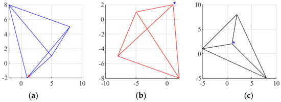
Figure 1.
Quaternion-pyramids for (a) the quaternion and its conjugates in (b) the (1,3)-model and (c) the (2,2)-model.
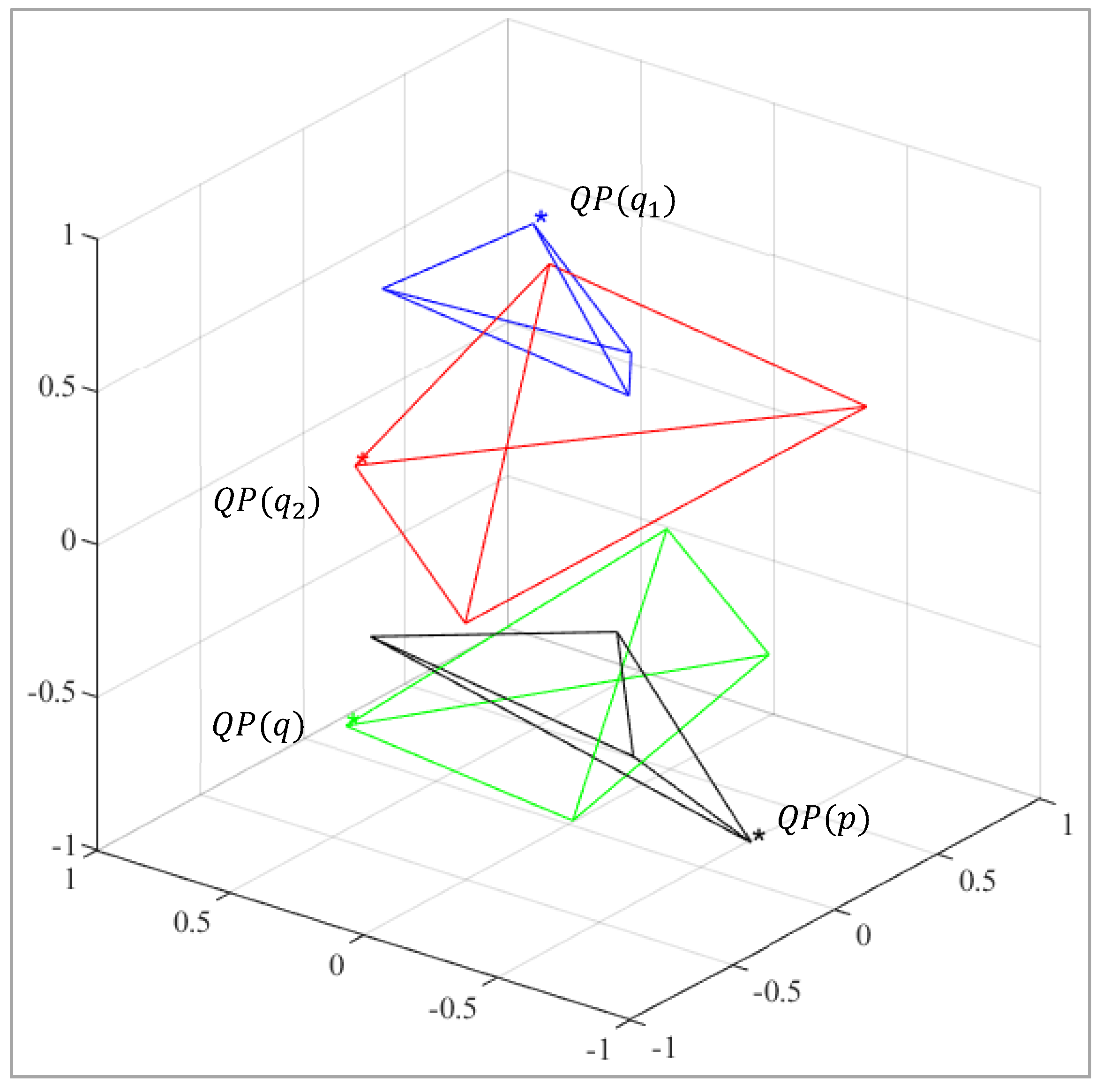
Figure 2 shows the following four pyramids. Two quaternions are considered, and The figure shows two pyramids and together with two pyramids for the quaternion multiplications . The first pyramid is calculated in the non-commutative (1,3)-model, and another in the commutative (2,2)-model, .
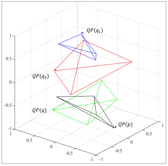
Figure 2.
Four quaternion-pyramids.
The following properties hold for the multiplication.
- The multiplication is commutative, .
- The multiplication unit is the quaternion . For this real unit for any quaternion .
- The multiplication rules of four quaternion units , and are given in Table 1. It should be noted that for two quaternion units and , the square is For the other two units and , the square is .
 Table 1. Multiplication table, .
 - The multiplication is associative, that is, for any quaternions , , and .
- The multiplication is distributive, that is, .
- The zero quaternion has “divisors.” For instance, the multiplication of two quaternions and is equal to
- The inverse to the non-zero quaternion is calculated by
- The inverse operation exists for all , except the quaternions of the form For quaternion exponential numbers, the inverse exists. As mentioned in [24], the absence of some inverse numbers is not an obstacle when using quaternions to process signals and color images.
- The division of quaternions and is calculated by .
- The multiplication of a quaternion on its conjugate is equal to the following quaternion:
- In the general case, is not a real number and cannot be used to define the modulus of the quaternion in the traditional sense. For example,
- The length, or modulus, of the quaternion is defined as , where the energy of the quaternion number is calculated by
Table 2 shows the main properties of quaternion numbers in the (1,3)- and (2,2)-models.
Table 2.
Main operations and properties of quaternions in two quaternion models.
3. The Quaternion Exponents in the (2,2)-Model
In this section, we describe the exponential functions in the (2,2)-model. For two pairs of quaternions and , the square . There are only two pairs of quaternions with the square equal to . For each of these quaternions, the exponential function is defined by the following series [22]:
Thus, there are four different exponential functions, or we can say two pair of quaternion exponential functions. The fundamental multiplicative property holds for these exponents, that is,
Now, we consider these two pairs of quaternion exponents.
1. The first pair of exponents is defined for the conjugate quaternions . The quaternion exponents are the following conjugate functions:
In the matrix form, the multiplication of a quaternion by the exponent is described as follows:
Here, we denote and With the operation of the Kronecker product of matrices, the above matrix of multiplication can be written as The matrix is the matrix of elementary rotation by the angle . Thus, the operation is reduced to separate rotations of two components of the quaternion, and , by the same angle.
2. The second pair of exponents is defined by the quaternion . The corresponding pair of quaternion exponential functions is
These two exponential functions are not conjugate but inverse to each other. The inverse of the exponent is In the matrix form, the multiplication of the exponent by a quaternion can be written as follows:
The matrix of the multiplication is the tensor product of the rotation matrix and the identity matrix, .
It should be noted that if we consider the symmetric matrix of the permutation (1,2), then the above two pairs of quaternion exponents can be derived from each as
4. Quaternion Discrete Fourier Transforms
In this section, we consider the concept of the quaternion discrete Fourier transform (QDFT) in the (1,3)- and (2,2)-models. In the first model, the -point QDFT of the quaternion signal is defined by
Here, is a pure quaternion unit number, such that As mentioned above, the number of such quaternions is infinite. For instance, this number can be taken as and . The multiplication is not commutative; therefore, this QDFT is the left-sided transform. The right-sided QDFT is defined as the sum of . The inverse -point QDFT is calculated by
The fast algorithms to calculate the QDFT exist for both types of transform in the 1D and 2D cases. For 2D signals, the QDFT can be defined as the right-, left-, or both-sided transform [14,24]. These transforms do not have one of the basic properties of the traditional Fourier transform, namely, the cyclic convolution of signals is not reduced to the operation of multiplication in the frequency domain. In the 1D case, the cyclic convolution of two periodic quaternion signals and is defined as
Here, we need to consider that , because the products . Thus, in the (1,3)-model, two different linear convolutions can be used.
Now, we consider these concepts in the (2,2)-model with two pairs of quaternion exponential functions, namely , when and . Each pair of these functions is used for the direct and inverse QDFTs. Thus, in the (2,2)-model there are only two pairs of the direct and inverse QDFTs. The (2,2)-model is commutative; therefore, the transform of the -point quaternion signal is defined as
Two different -point QDFTs are described in the following way.
- When the quaternion is and the angle is , the basis exponential functions are
The -point direct QDFT is defined as
or
Here, and are the traditional -point DFTs of the complex signal and , respectively,
This -point QDFT is called the -point -QDFT and it requires two -point DFTs [22]. The inverse -point -QDFT is calculated by
- 2.
- In the case, the basis exponential functions for the QDFT are
The -point QDFT which is called the -point -QDFT is defined as [22]
In the matrix form, this transform can be written with the rotation matrices as
The inverse -point -QDFT is calculated by
Thus, in the (2,2)-model, we can work with only two -point QDFT, namely, -QDFT and -QDFT.
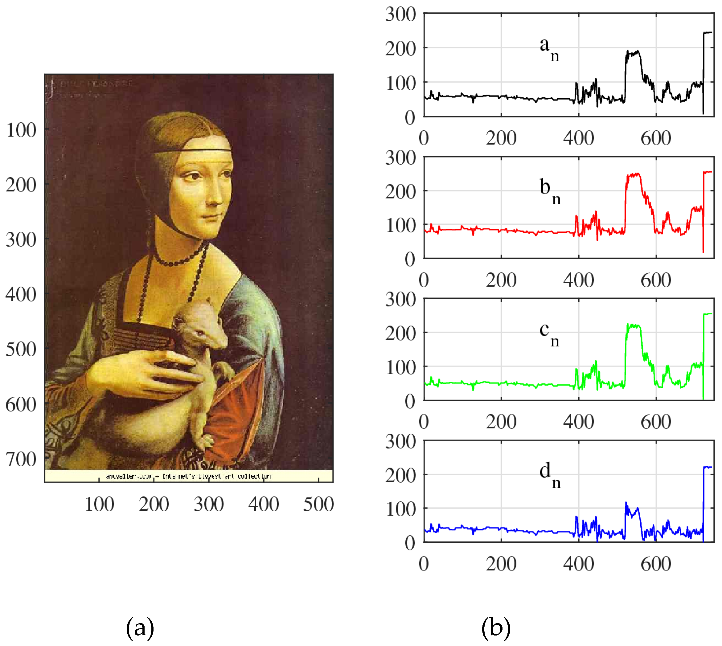
As an example, Figure 3 shows the color image ‘leonardo9.jpg’ of 744 526 pixels in part (a) and the quaternion signal composed from column number 101 in part (b). The signals , and are the red, green, and blue channels of the image column, respectively. The signal is the average of these signals.
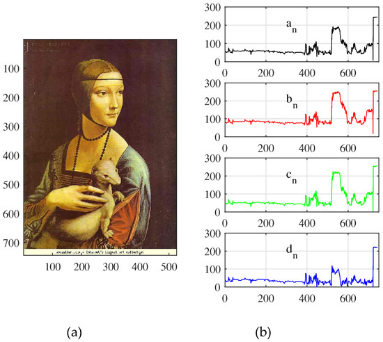
Figure 3.
(a) The color image and (b) the quaternion signal of length 744 composed from one image column.
The -QDFT and -QDFT of this quaternion signal are plotted in absolute scale, | in Figure 4 in parts (a) and (b), respectively. The difference between these two plots is shown in part (c).
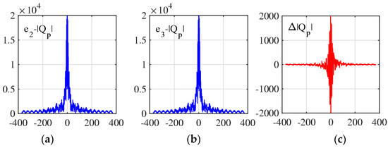
Figure 4.
The magnitude of (a) the -QDFT, (b) the -QDFT, and (c) the difference of these transforms.
As shown in [22], in the (2,2)-model, the aperiodic convolution of quaternion signals can be calculated by multiplying the QDFTs. This statement is valid for both types of QDFT. The convolution of a periodic quaternion signal with another one is unique,
Here, the subscripts are considered by modulo . This convolution is calculated by four complex convolutions as follows:
For and 3, the -point -QDFT of the convolution is calculated by , Here, and are components of the corresponding -point -QDFT of signals and , respectively. What type of QDFT is used for computing the aperiodic convolution is irrelevant. We think that the calculation of the quaternion convolution by the -QDFT is simple. According to the multiplication, the -QDFT of the aperiodic convolution is calculated by
Therefore, the task of calculating the quaternion aperiodic convolution in the frequency domain is solved in the (2,2)-model. In the traditional (1,3)-model of quaternions, this problem does not have such a simple solution—it is unsolvable. Table 3 summarizes the above considerations.
Table 3.
Properties of aperiodic convolution and QDFT.
5. Processing Images in the (2,2)-Model
In this section, we describe the concept of the 2D QDFT of images, which will be used in color image enhancement, namely, in the method which is called alpha-rooting. A color image in the RGB model will be presented by the quaternion image and then transformed to the frequency domain. Let be components of the primary colors, red (R), green (G), and blue (B), in the image of pixels. To compose the quaternion image , we add the real component . Thus, . The real part of this image is usually considered zero, , or the gray-scale component at each pixel (. The brightness of the image can also be considered, . In the (2,2)-model, the quaternion image is the pair of 2D data and In many applications, processing color images in quaternion space is efficient, since at each pixel the color triplet (plus the gray) is treated as one number, quaternion. Note that in the traditional approach, each color component of the image is processed separately. And this causes many unwanted effects on colors in the processed images [5,14].
The two-dimension -point QDFT in the frequency-point is calculated by
where In the (1,3)-model, two sums in this equation are different transforms; the first one is called the separable right-sided 2D QDFT [21,24].
We consider the 2D QDFT, which is calculated by the 1D -QDFTs. This 2D transform is called the 2D -point -QDFT—the case when [22,25]. As in the 1D case, the 2D -QDFT has a simple form, when compared with the 2D -QDFT. The 2D -QDFT of the quaternion image is calculated by
Here, and are the -point 2-D DFTs of the complex components and , respectively,
Thus, the calculation of the -point -QDFT is reduced to two 2D DFTs. The inverse -point -QDFT is calculated by
5.1. Method of Alpha-Rooting by the 2D QDFT
The absolute value, or the module, of the quaternion is defined as In the alpha-rooting [26,27], the image is enhanced by changing its absolute value at each frequency point to , where the parameter is from the interval (0,1). Given value , the 2D -QDFT of the quaternion image is processed as follows:
Here, is a necessary constant, since the alpha-rooting method reduces the transforms in absolute scale.
The main steps of the algorithm:
- Compose the quaternion image from the given RGB color image, .
- Calculate the 2D -QDFT of the quaternion image, .
- Calculate the module of the transform,
- Process the transform modules by the alpha-rooting, .
Thus, the 2D -QDFT of the quaternion image changes by the non-negative coefficients
- 5.
- Calculate the inverse 2D -QDFT, .
- 6.
- Multiply the image by the constant to raise the range of the image.The output of the alpha-rooting is the quaternion image Rounding to integers is required.
- 7.
- Compose the new color image, , as the three-component imaginary part of the quaternion image .
- 8.
- Extract the new grayscale image from the quaternion image , as its real part. Note that this grayscale image is not the gray or brightness of the new color image .
The new image is parameterized by . Therefore, the question arises as to how to choose the value of this parameter to better enhance the color image. As our preliminary examples have shown, the choice of the best values of for enhancing color and quaternion images can be based on the known measure of color image enhancement (EMEC) [5,13]. This measure is used before and after image processing. The EMEC is the generalization of the enhancement measure that was used for grayscale images.
- A.
- Enhancement measures for grayscale images
To estimate the quality of grayscale images, we effectively developed and used the concept of the quantitative estimated measure of enhancement (EME). This measure was selected after analyzing the Weber and Fechner laws of the human visual system [28,29]. The measure is defined as the average of the range of image intensity in the logarithm scale when it is divided by blocks of the same size , for example, Only the full blocks are considered. Therefore, the number of blocks inside a discrete image of pixels is calculated as , where , and denotes the rounding floor function. The EME of the image is
Here, inside the th block, the maximum, , and minimum, , of the image are calculated. Thus, the EME of the image is estimated block-wise by using the logarithm range of the image. If all values of the image in a block are 0, this block can be removed from the measure calculation. To avoid such cases, can be calculated instead. The change does not change the quality of the image unless it is binary.
Together with EME, other contrast measures also can be used, including [14]:
- The estimated measure of enhancement entropy measure (EMEE)
- 2.
- The Michelson enhancement measure (MEM)where the Michelson visibility ratio is calculated by
- 3.
- The signal-noise ratio (or the ratio of the mean of the image and standard deviation)where
Our experimental results show that the EME and EMEE measures can be effectively used in enhancing images. After processing the image, , the EME of the enhanced image is calculated and compared with the EME of the original image. The range of the alpha-rooting image is usually smaller than [0,255]. Therefore, the obtained image should be multiplied by a coefficient. The new image and its quality depend on the value of parameter , i.e., and the measure is a function of that is, The parameters of interest for alpha-rooting are in the range The degree of enhancement is determined by the EME measure. The best or optimal values of the enhancement are considered to be the values , for which or
To illustrate the introduced above measures of image enhancement, we consider the image of pixels shown in Figure 5 in part (a). The histogram of the image is given in part (b). The enhancement by the Fourier transform-based alpha-rooting was used when changing the parameter α in the interval [0,1] with a step of 0.01. The graph of the measure of this image, , as the function of is shown in part (c). Blocks of size were used to calculate the EME. For the original image, the measure of enhancement equals 7.63. The maximum of the function is at point and equals . The image enhanced by the -rooting is shown in part (d). It was multiplied by the coefficient 19 to scale the image. In parts (e) and (f), the graph of the measure and the enhanced image by the -rooting (and multiplied by 17) are shown, respectively. This measure has the maximum 1071.26 at point The measure of the original image equals The best parameters and for these two measures are very close to each other, as well as the results of the enhancement, which are shown in parts (d) and (f). The function is much smoother than the measure, and its graph has a distinct peak. For other images, the optimal values of the parameter may be very different, but the smoothness of the function ) is preserved and easier to work with.
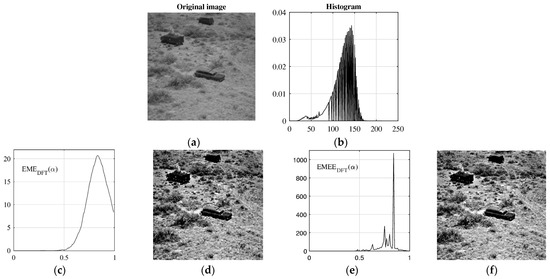
Figure 5.
(a) The image ‘7.1.10.tiff’ (from http://sipi.usc.edu/database, accessed on 22 January 2025), (b) the histogram of the image, (c) the EME function, (d) the enhanced image by the 0.83-rooting. (e) The graph of the EMEE function and (f) the image enhanced by the 0.84-rooting method.
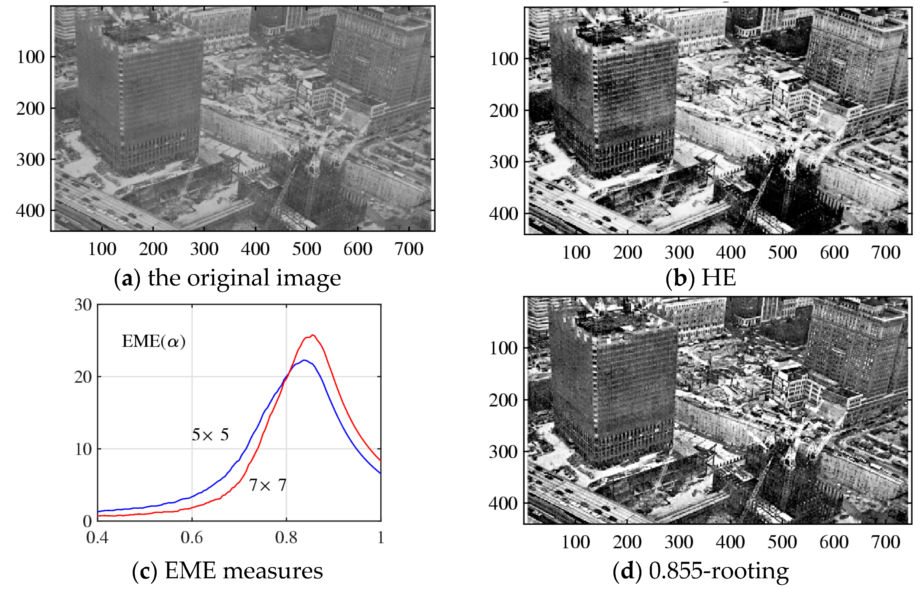
In Figure 6a, the image of 440 750 pixels is shown, as well as the result of the histogram equalization (HE) of the image in part (b). The graph of the enhancement measure , when processing by the alpha-rooting, is given in part (c). The measure function was calculated by dividing the image by blocks of sizes 5 × 5 and 7 × 7. The parameter for the α-rooting method of enhancement varies in the interval [0.4,1] with a step of 0.005. Two graphs of the enhancement measure EME have pikes at the point and 0.855, for the 5 × 5 and 7 × 7 block sizes, respectively. These values are almost the same, and we consider for the best visual estimation of the enhancement. The EME of the original image equals 8.30 and 25.76 for the 0.855-rooting enhancement, which is shown in part (d). There, the enhancement can be estimated as . One can note the high quality of the 0.855-rooting image in comparison with the HE image in part (b).
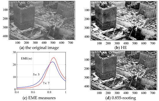
Figure 6.
(a) The original grayscale image and (b) enhanced image by (b) histogram equalization. (c) Two EME measures of alpha-rooting method, and (d) the 0.855-rooting of the image.
To estimate the quality of color images, we consider the color image enhancement measure (EMEC). For a color image after division by blocks of size each, for instance , the measure is calculated by
Here, is the number of blocks, and and are the maximum and minimum values in the -th image block, respectively.
- B.
- Alpha-rooting components-wise
Color images in the RGB color model can be separately processed by red, green, and blue colors. This is the traditional method of processing color images. In the alpha-rooting enhancement, each color component can be processed by alpha-rooting with different or the same values of parameters and . We call this method -rooting of the color image For images in the HSI color model, with hue (H), saturation (S), and intensity (I) components, only the last component, intensity, will be only processed by alpha-rooting. The first two components, hue and saturation will stay the same.
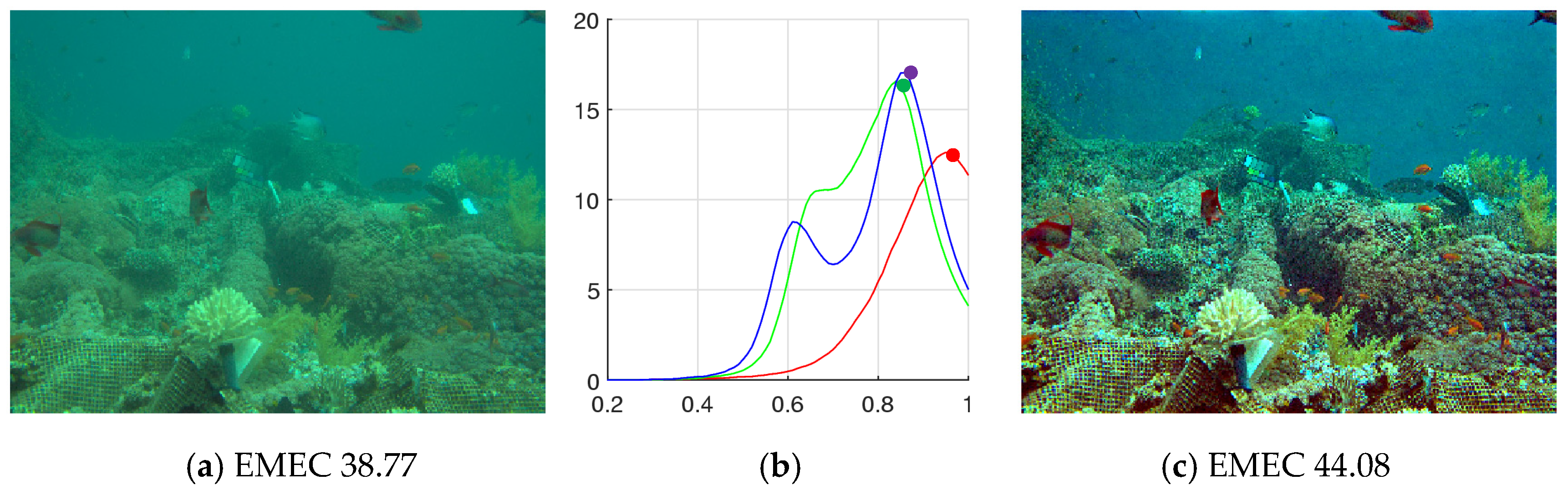
To choose values of these parameters, we can use, for instance, the EME measure. As an example, Figure 7 shows the 1516 2012-pixel underwater RGB image in part (a) with EMEC of 38.77, which was calculated by blocks of size 5 In part (b), the graphs of functions of the red, green, and blue channels are shown. The parameter of runs the interval [0.2,1]. The maximum values of these functions are at points and The color image composed of -rooting of red, 0.83-rooting of green, and 0.84-rooting of blue components is shown in part (c). The enhancement measure of this image equals EMEC = 44.08.
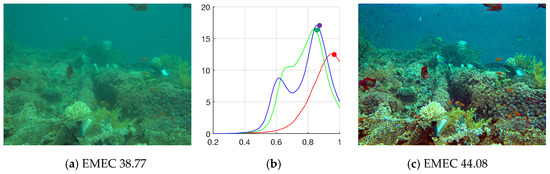
Figure 7.
(a) The original image, (b) EMEs of red, green, and blue components, and (c) enhanced image.
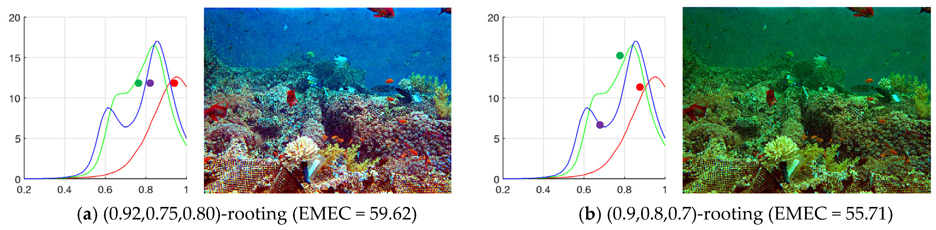
Since the color components are processed separately, it is not possible to state that the above (094,0.84,0.83)-rooting results in the highest enhanced image. It is possible to select other triplets of the vector parameter and obtain images that we can consider the best. As examples, Figure 8 shows two enhanced images together with the graphs of the EMEs of three color channels, R, B, and B. The values of alpha parameters for these channels are marked on the graphs. The case with equal EME for all color channels is shown in part (a). The EMEC of the color image is of 59.62, which is the highest number for all considered cases. Also, a good, enhanced color image is shown in part (b) for the vector parameter (0.9,0.8,0.7).

Figure 8.
(a) and (b) Two enhanced images.
- C.
- Comparison with HE and Retinex
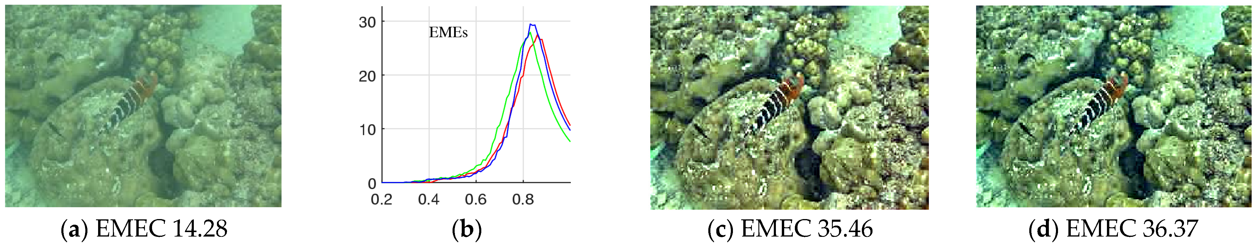
The methods of histogram equalization (HE) [30,31,32] and Retinex [33,34,35,36,37] are widely used in color image enhancement. We consider these methods together with the method of alpha-rooting. The underwater RGB color image of 192 262 pixels is shown in Figure 9 in part (a). This image has a measured EMEC of 11.26, which was calculated by blocks 5 5. The graphs of EME of three colors are given in part (b), with maximum values at points 0.85, 0.82, and 0.82, for the red, green, and blue channels, respectively. The corresponding (0.85,0.82,0.82)-rooting of this image with an EMEC of 35.46 is shown in part (c). In part (d), the (0.82,0.82,0.82)-rooting is shown with an EMEC of 36.37.
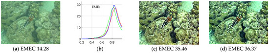
Figure 9.
(a) The original image, (b) EMEs of red, green, and blue components, and enhanced images by (c) (0.85,0.82,0.82)-rooting and (d) (0.82,0.82,0.82)-rooting.
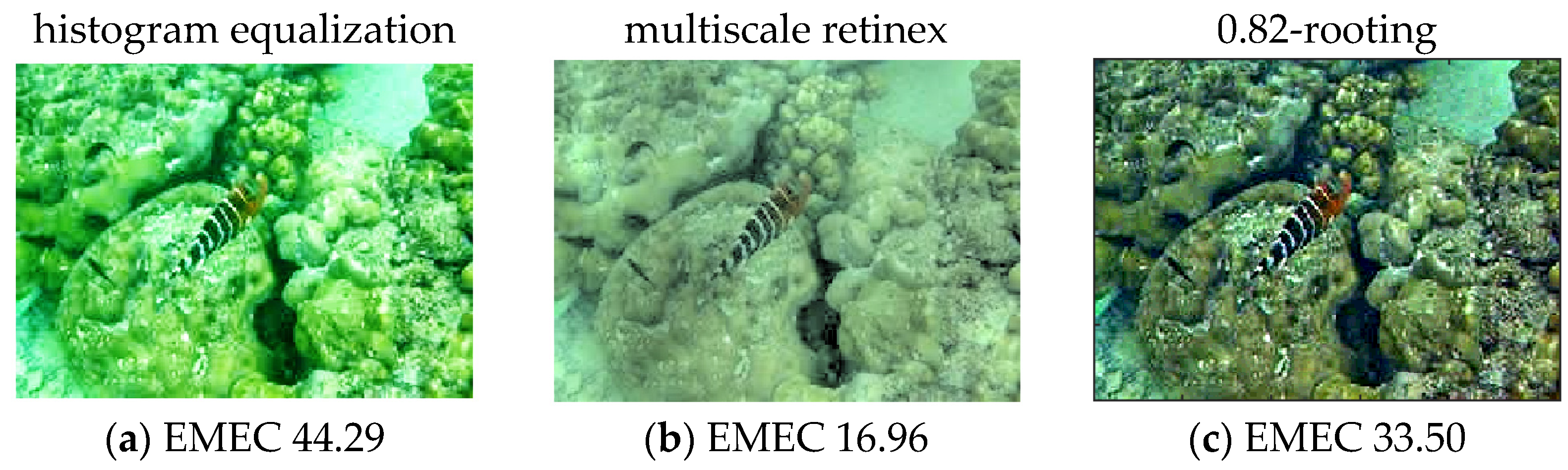
Figure 10 shows the result of the histogram equalization with a measured EMEC of 44.29 in part (a). The result of image enhancement by the multi-retinex is shown in part (b). The image was normalized, and sizes of the Gaussian filters were taken 7, 15, and 21 as suggested [33]. The retinex enhancement has an EMEC of 16.96. One can see that the enhancement of the color image was not achieved in these two methods. For comparison, we also add the result of the color image enhancement by the 0.82-rooting. The result is shown in part (c). One can see good enhancement of the image; the color measure of enhancement equals 33.50. Measures of EMEC and EME were calculated by blocks of 5 5 pixels.
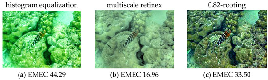
Figure 10.
Color image enhancement by (a) histogram equalization (MATLAB’s version), (b) multi-retinex algorithm (the original version [33]), and (c) method of 0.82-rooting.
The quaternion image enhancement (EMEQ) measure for a quaternion image is calculated similarly [27],
This measure includes the real part of the quaternion image. The measure EMEQ is calculated for the input quaternion image and the processed image . In most cases, the best parameter for color enhancement is considered the value of with a maximum of and (or minimum). Our experimental results show that the measures EMEC and EMEQ are effective in selecting the best parameters to receive color images with high quality [27]. Other measures for selecting the best values of and estimating color image quality after image processing can also be used. We mention the color image contrast and quality measures [14].
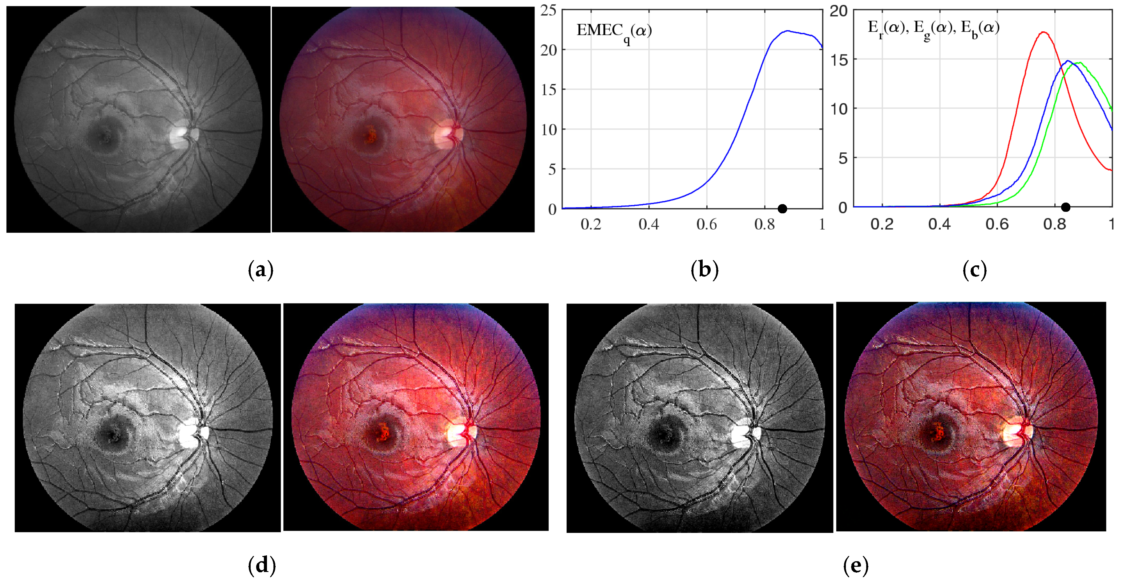
As an example, Figure 11 shows the quaternion image of 877 1024 pixels in part (a). The grayscale image is the real part, and the color image is the imaginary part of the quaternion image. The graph of the EMEC measure as the function of is shown in part (b). The maximum of this function is at point 0.879. In part (c), the graphs of the measured EME of the color channels are given. The point was selected, at which these graphs roughly intersect. The quaternion images after 0.879 and 0.82-rooting enhancements are shown in parts (d) and (e), respectively.
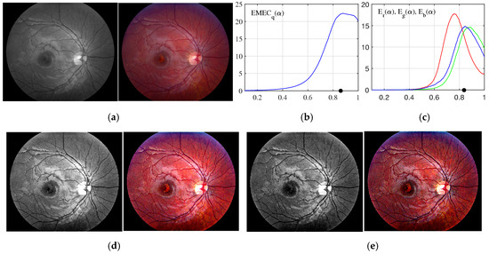
Figure 11.
(a) The quaternion fundus image, (b) the graph of the EMEC function calculated for -rooting by the 2-D QDFT, (c) the graphs of EME functions calculated for red, green, and blue channels of the -rooting. The enhanced quaternion after (d) 0.879-rooting and (e) 0.82-rooting.
5.2. The Separable Alpha-Rooting
The alpha-rooting method by the QDFT can be modified in the following two ways.
- The separable 1-parameter alpha-rooting of the quaternion image is the method of processing the 2D -QDFT of the image as
- The 2-parameter alpha-rooting of the quaternion image uses two parameters and from the interval to process the 2D -QDFT of the quaternion image as follows:
In the case, the 2-parameter alpha-rooting coincides with the 1-parameter alpha-rooting.
5.3. Alpha-Rooting of Color Images and the (1,3)-Model
In the (1,3)-model, we consider one of the 2D QDFTs, namely, the separable right-sided 2D QDFT [27]. This transform of the quaternion image is calculated by
Here, and are pure quaternion units. The transform uses 1D QDFTs by rows and then 1D QDFT by columns. Given quaternion signal and a pure quaternion , the 1D QDFT, , with the basis exponential functions requires four traditional DFTs since it is calculated by [14]
and are the DFTs of the components , and , respectively. and denote the operations of real and imaginary parts of the complex number , respectively. The multiplication of the 4D vector by the matrix requires a maximum of 12 real multiplications. In the case, when and , the exponential basis functions are and The matrices of multiplication have simple forms,
and the corresponding 1D QDFTs are calculated by
These -point QDFTs require four 1D DFTs plus additions. In this case, the right-sided 2D QDFT of the quaternion image is calculated by
A total of 1D QDFTs plus additions are used to calculate the 2D QDFT. The inverse 2D right-sided QDFT is calculated by
The complexity of the QDFTs in the (1,3) and (2,2)-models for images of pixels is described in Table 4.
Table 4.
Complexity of the calculations for the two algebras.
The main steps of the algorithm for -rooting in the (1,3)-model:
- Compose the quaternion image from the color RGB image .
- Calculate the right-sided 2D QDFT, of the quaternion image.
- Given , calculate the coefficients .
- Modify the 2D QDFT as .
- Calculate the inverse 2D QDFT .
- Select the best value for color image enhancement by using the measures EMEQ or EMEC.
6. Experimental Results with Color Images
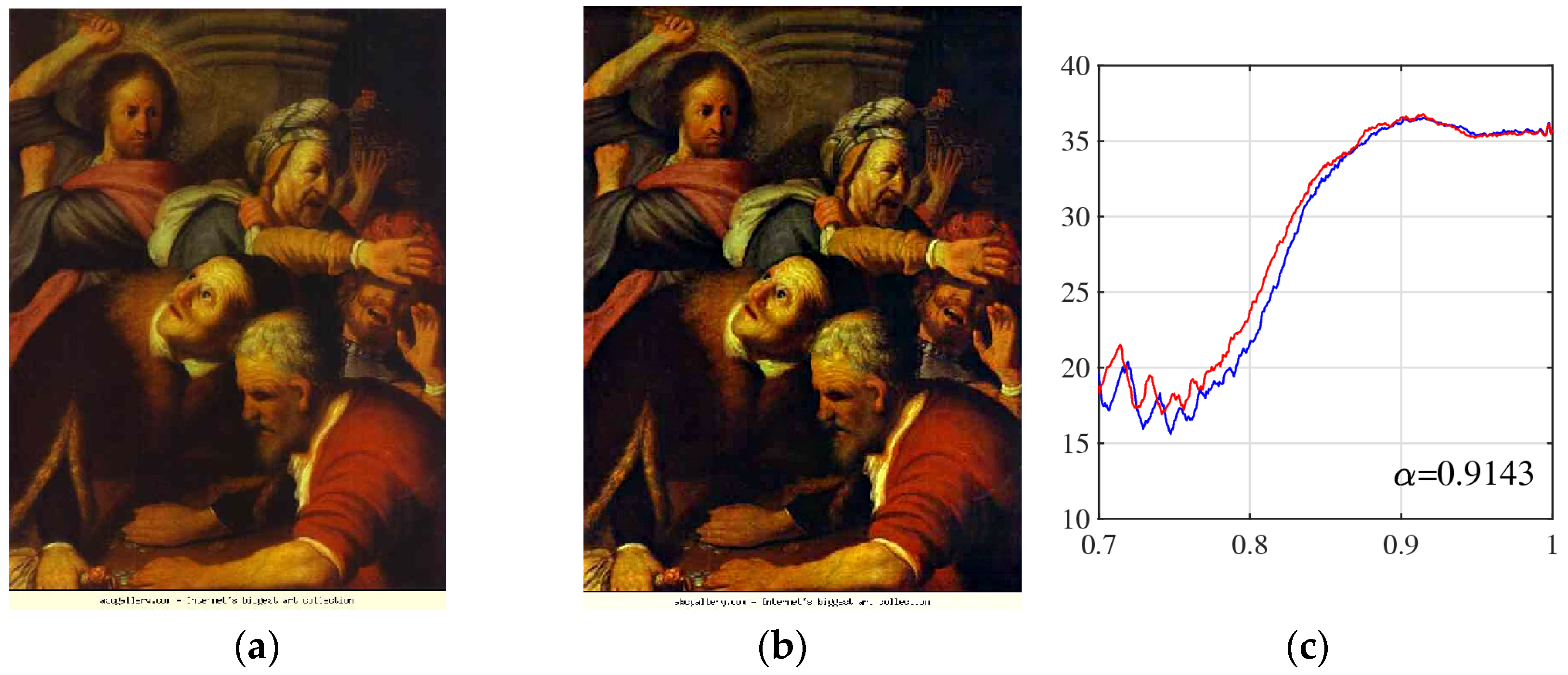
In this section, a few illustrative examples of the 2D QDFT-based alpha-rooting are presented. Many color images of art in this paper are from Olga’s Gallery—Free Art Print Museum by address https://www.freeart.com/gallery/ (accessed on 22 January 2025) with permission to use them in our research. Figure 12 shows the RGB color image ‘rembrandt195.jpg’ in part (a) and the enhanced image in part (b). The enhanced image was calculated by the alpha-rooting with -QDFT, when the parameter This value of the parameter is considered optimal, or best, according to the EMEC measure calculated by Equation (39) with block size 7 7. This measure as the function EMEC() has a maximum of 36.54 at this point. The measure of the original image is EMEC.
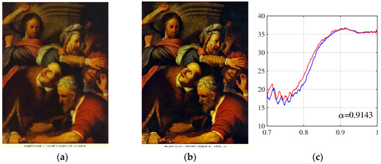
Figure 12.
(a) The original image, (b) 2D e2-QDFT based 0.9143-rooting (with the scaling factor of ), and (c) the two curves of the EMEC.
Two EMEC functions are shown in Figure 12 in part (c); they are close to each other, and both achieve the maximum at the same point. The first graph (which is a little higher than the other one) was calculated by the 2D -QDFT-based alpha-rooting described in Section 5.1, when the transform is modified as , The second graph is for the EMEC measure calculated from the 1-parameter alpha-rooting described in Section 5.2, when the -QDFT of the images is processed as follows: , Figure 13 shows the enhanced image by 1-parameter 0.9143-rooting in part (a). For comparison, the 0.9143-rooting of the image by the 2D QDFT in the (1,3)-model is shown in part (b).
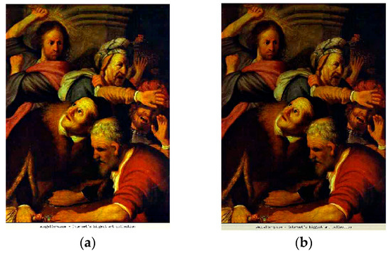
Figure 13.
The enhanced images of the 0.9143-rooting: (a) in the (2,2)-model and (b) in the (1,3)-model.
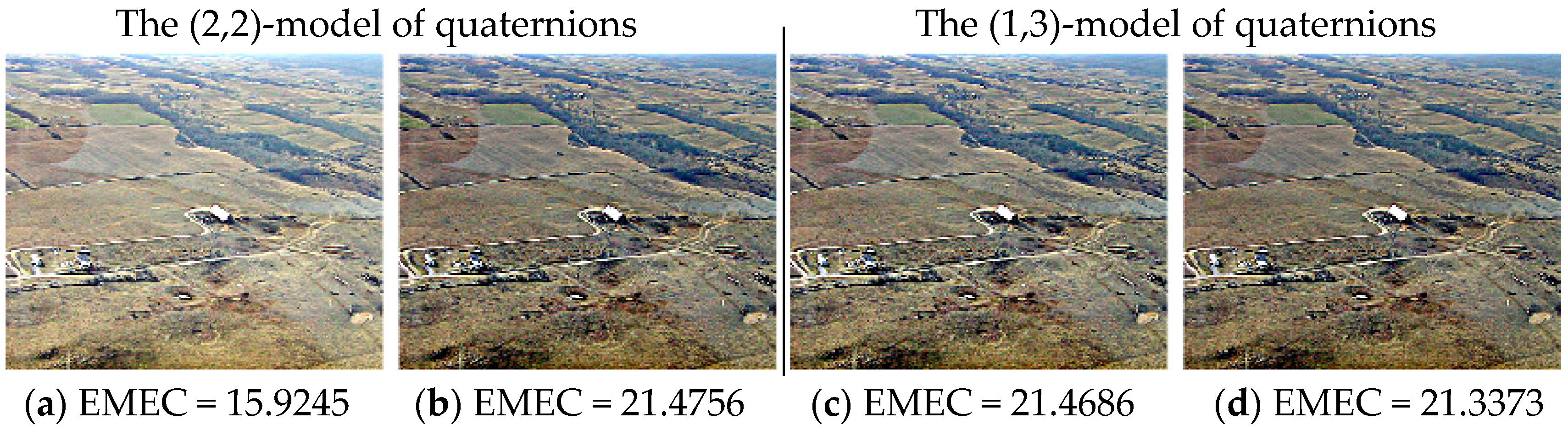
Below are a few results of processing other color images by the alpha-rooting and separate algorithms of the alpha-rooting in the commutative (2,2)-model. The results of image enhancement by the alpha-rooting in the non-commutative (1,3)-model are also shown. Figure 14 shows the results of the 0.92-rootings, when processing the image of San Antonio. The values of the color image enhancement EMEC are shown.
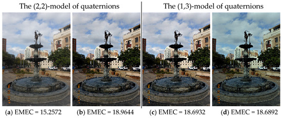
Figure 14.
(a) The original color image. The enhanced images in the (2,2)-model by (b) the main 0.92-rooting and (c) separable 1-parameter 0.92-rooting. (d) The 0.92-rooting in the (1,3)-model.
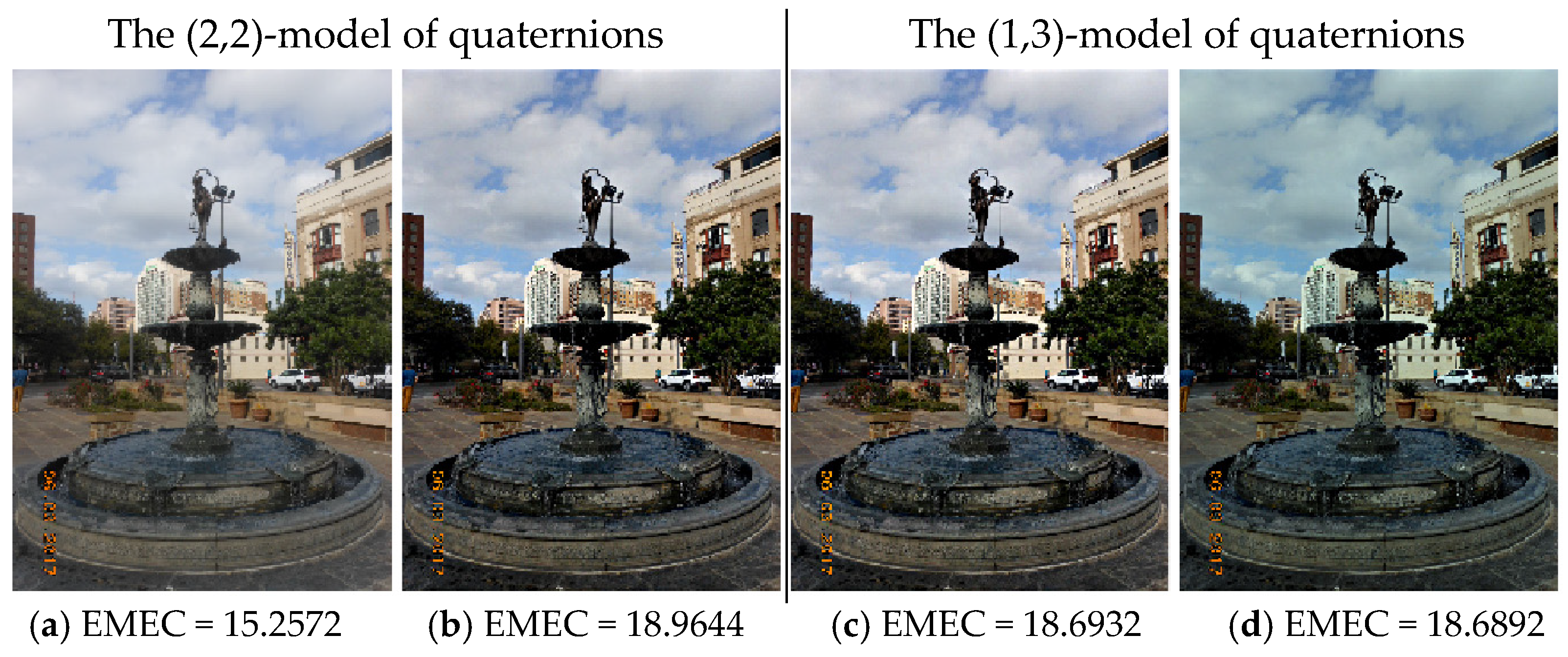
Figure 15 shows the results of the same methods of the 0.92-rootings, when processing another image of San Antonio. One can note that the images processed in the (2,2)-model have higher values of EMEC.
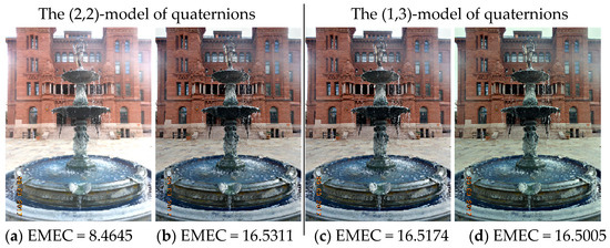
Figure 15.
(a) The original color image. The enhanced images in the (2,2)-model by (b) the main 0.92-rooting and (c) separable 1-parameter 0.92-rooting. (d) The 0.92-rooting in the (1,3)-model.
Figure 16 shows the results of processing image ‘image13-2.jpg.’ The method of alpha-rooting works well in both models for many images. It means that the (2,2)-model does not perform any worse but in fact better than another model, that is, the (1,3)-model.

Figure 16.
(a) The original color image. The enhanced images in the (2,2)-model by (b) the main 0.92-rooting and (c) separable 1-parameter 0.92-rooting. (d) The 0.92-rooting in the (1,3)-model.
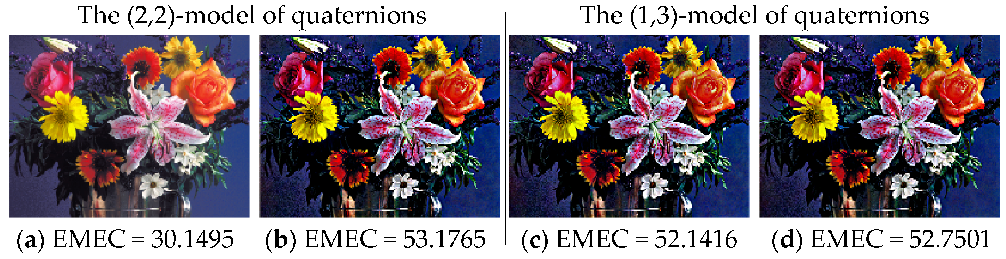
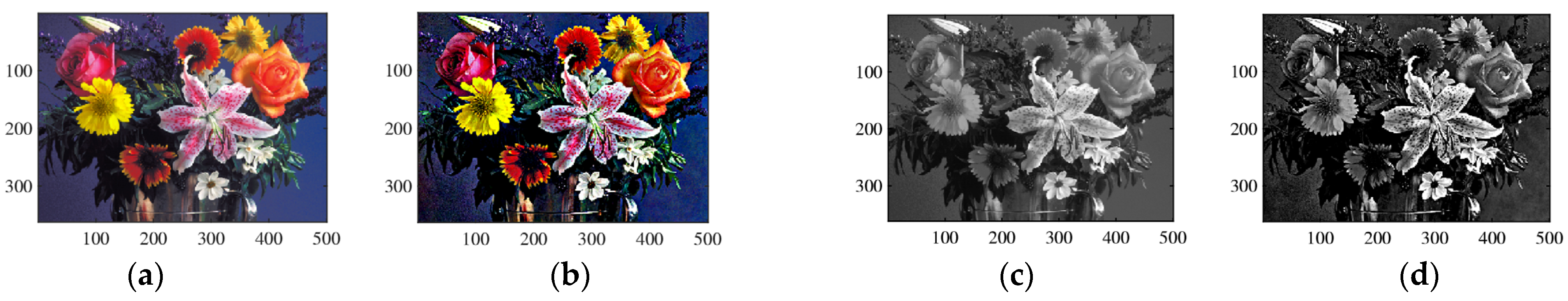
The results of processing the well-known “flowers” image are shown in Figure 17 in parts (a)–(d).
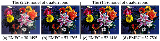
Figure 17.
(a) The original color image. The enhanced images in the (2,2)-model by (b) the main 0.92-rooting and (c) separable 1-parameter 0.92-rooting. (d) The 0.92-rooting in the (1,3)-model.
Now we apply the method of alpha-rooting in the (2,2)-model, when two parameters and are used and the 2D QDFT of the color image is processed as
Figure 18 shows results of the color image enhancement processing by the 2-parameter alpha-rooting with different sets of parameters and . In part (b), the image of San Antonio was processed by the parameters The enhancement by parameters and is shown in part (c).
Figure 18.
(a) The original color image, and (b) the [0.92,0.92]-rooting, and (c) the [0.92,0.93]-rooting in the (2,2)-model.
It should be noted that when processing color images in the quaternion models, the color image is only the imaginary part of the quaternion image. The enhancement of quaternion image includes two images, the color one and the gray one. They are processed together. The first component of the quaternion image, which is referred to as the grayscale image is not the grayscale image of the processed color image. The enhancement of quaternion image results in the enhancement of both images. As examples, we consider a few color images processed in the (2,2)-model by the 2-D -QDFT-based alpha-rooting.
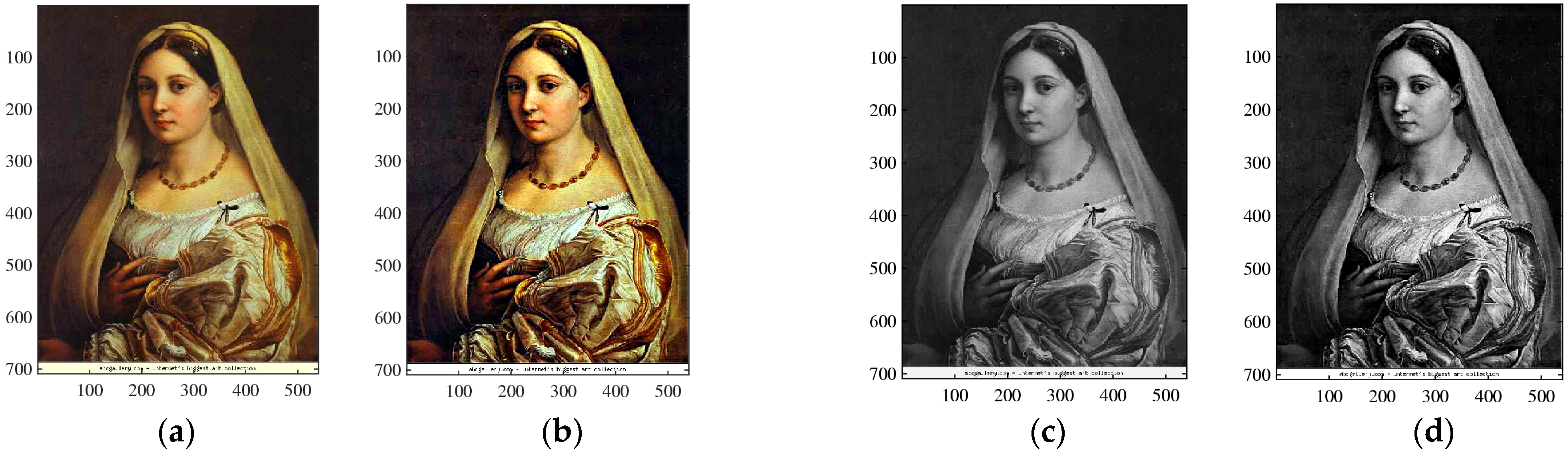
Figure 19 shows the color image ‘raphael155.jpg’ in part (a), which was embedded in the quaternion image as its imaginary part. The imaginary component (the new color image) of the enhanced quaternion image by the 0.92-rooting is shown in part (b). The grayscale image of the original color image is shown in part (c). The real part of the processed quaternion image is shown in part (d). This image is not the average of colors in the image in part (b). Thus, both grayscale and color images were enhanced when processing the quaternion image.

Figure 19.
(a) The original color image and (c) its grayscale image. The processed (b) imaginary and (d) real components of the enhanced quaternion image by the -QDFT 0.92-rooting.
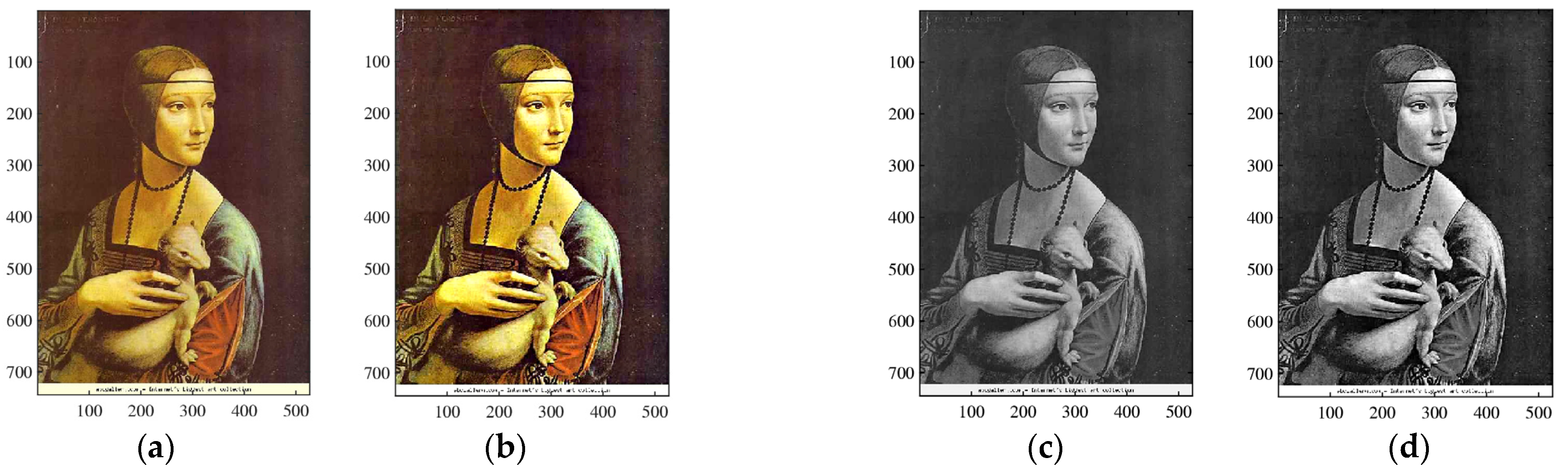
Figure 20 and Figure 21 show the results of enhancement of the quaternion images when the color images ‘leonardo9.jpg’ and ‘flowers’ were used, respectively.
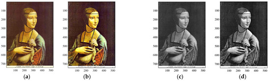
Figure 20.
(a) The original color image ‘leonardo9.jpg’ and (c) its grayscale image. The processed (b) imaginary and (d) real components of the enhanced quaternion image by the -QDFT 0.92-rooting (4).
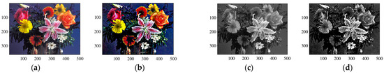
Figure 21.
(a) The original color flowers image and (c) its grayscale image. The processed (b) imaginary and (d) real components of the enhanced quaternion image by the -QDFT 0.80-rooting ().
7. Conclusions
New quaternion algebra, the (2,2)-model, was presented, and new methods of alpha-rooting by the quaternion discrete Fourier transform (QDFT) were described and analyzed in this model. The main properties of this model were considered. This model of quaternions is commutative and associative and allows to calculate the aperiodic convolution of quaternion images in the frequency domain. The results of the image enhancement of color images in this model were compared with the alpha-rooting in the traditional (1,3)-model. The comparison with the known methods of histogram equalization and Retinex is also provided with examples. The preliminary experimental examples show the effectiveness of the proposed methods for color image enhancement by the 2D QDFT. We believe that the commutative (2,2)-model together with the non-commutative (1,3)-model can be effectively used in color image enhancement, as well as other areas of color imaging. The proposed methods of alpha-rooting are fast, because of fast 1D and 2D QDFTs, and do not require much memory, as well as machine learning algorithms, which require much time and memory and do not work well on many images presented in this work.
Author Contributions
Conceptualization, A.M.G.; methodology, A.M.G.; software, A.M.G. and A.A.G.; validation, A.M.G.; formal analysis, A.M.G. and A.A.G.; investigation, A.M.G.; resources, A.M.G.; data curation, A.M.G.; writing—original draft preparation, A.M.G.; writing—review and editing, A.M.G. and A.A.G.; visualization, A.M.G. and A.A.G.; supervision, A.M.G.; project administration, A.M.G. All authors have read and agreed to the published version of the manuscript.
Funding
This research received no external funding.
Data Availability Statement
The original contributions presented in this study are included in the article. Further inquiries can be directed to the corresponding author(s).
Acknowledgments
This article is a revised and expanded version of Ref. [25], which was presented at SPIE 13033 Conference, Defense + Commercial Sensing 2024, National Harbor, MD 20745, USA, 22 April 2024.
Conflicts of Interest
The authors declare no conflicts of interest.
References
- Harris, J.L. Constant variance enhancement: A digital processing technique. Appl. Opt. 1977, 16, 1268. [Google Scholar] [CrossRef] [PubMed]
- Wang, D.C.; Vagnucci, A.H.; Li, C.C. Digital image enhancement: A survey. Comput. Vis. Graph. Image Process. 1983, 24, 363–381. [Google Scholar] [CrossRef]
- Trussell, H.J.; Saber, E.; Vrhel, M. Color image processing [basics and special issue overview]. IEEE Signal Process. Mag. 2005, 22, 14–22. [Google Scholar] [CrossRef]
- Gonzalez, R.C.; Woods, R.E. Digital Image Processing, 4th ed.; Pearson: New York, NY, USA, 2018. [Google Scholar]
- Grigoryan, A.M.; Agaian, S.S. Image processing contrast enhancement. In Wiley Encyclopedia of Electrical and Electronics Engineering; Webster, J.G., Ed.; Wiley: Hoboken, NJ, USA, 2017; pp. 1–22. [Google Scholar]
- Nithyananda, C.R.; Ramachandra, A.C.; Preethi. Survey on histogram equalization method-based image enhancement techniques. In Proceedings of the 2016 International Conference on Data Mining and Advanced Computing (SAPIENCE), Ernakulam, India, 16–18 March 2016; IEEE: New York, NY, USA, 2016; pp. 150–158. [Google Scholar]
- Han, J.-H.; Yang, S.; Lee, B.-U. A novel 3-D color histogram equalization method with uniform 1-D gray scale histogram. IEEE Trans. Image Process. 2011, 20, 506–512. [Google Scholar] [CrossRef] [PubMed]
- Trahanias, P.E.; Venetsanopoulos, A.N. Color image enhancement through 3-D histogram equalization. In Proceedings of the 11th IAPR International Conference on Pattern Recognition, The Hague, The Netherlands, 30 August–3 September 1992; IEEE Comput. Soc. Press: Washington, DC, USA, 1992; Volume IV, pp. 545–548. [Google Scholar]
- Pitas, I.; Kiniklis, P. Multichannel techniques in color image enhancement and modeling. IEEE Trans. Image Process. 1996, 5, 168–171. [Google Scholar] [CrossRef] [PubMed]
- Mlsna, P.A.; Zhang, Q.; Rodriguez, J.J. 3-D histogram modification of color images. In Proceedings of the 3rd IEEE International Conference on Image Processing, Lausanne, Switzerland, 16–19 September 1996; IEEE: New York, NY, USA, 1996; Volume 3, pp. 1015–1018. [Google Scholar]
- Land, E.H.; McCann, J.J. Lightness and retinex theory. J. Opt. Soc. Am. 1971, 61, 1–11. [Google Scholar] [CrossRef]
- Land, E. An alternative technique for the computation of the designator in the retinex theory of color vision. Proc. Natl. Acad. Sci. USA 1986, 83, 3078–3080. [Google Scholar] [CrossRef] [PubMed]
- Agaian, S.S.; Panetta, K.; Grigoryan, A.M. Transform-based image enhancement algorithms with performance measure. IEEE Trans. Image Process. 2001, 10, 367–382. [Google Scholar] [CrossRef] [PubMed]
- Grigoryan, A.M.; Agaian, S.S. Quaternion and Octonion Color Image Processing with MATLAB; SPIE Press: Bellingham, WA, USA, 2018. [Google Scholar]
- Gauss, C.F. Mutationen des raumes [transformations of space] (c. 1819). In Carl Friedrich Gauss Werke, 8th ed.; Brendel, M., Ed.; Teubner: Stuttgart, Germany, 1900; pp. 357–361. [Google Scholar]
- Hamilton, W.R. On a new species of imaginary quantities connected with a theory of quaternions. Proc. R. Ir. Acad. 1844, 2, 424–434. Available online: https://www.emis.de/classics/Hamilton/Quatern1.pdf (accessed on 27 December 2024).
- Hamilton, W.R. Elements of Quaternions; Longmans, Green & Co.: London, UK, 1866. [Google Scholar]
- Kantor, I.L.; Solodovnikov, A.S. Hypercomplex Numbers; Nauka: Moscow, Russia, 1973. [Google Scholar]
- Bülow, T. Hypercomplex Spectral Signal Representations for the Processing and Analysis of Images; Christian-Albrechts-Univ.: Kiel, Germany, 1999; Volume 9903, p. 171. [Google Scholar]
- Yin, Q.; Wang, J.; Luo, X.; Zhai, J.; Jha, S.K.; Shi, Y.-Q. Quaternion convolutional neural network for color image classification and forensics. IEEE Access 2019, 7, 20293–20301. [Google Scholar] [CrossRef]
- Sangwine, S.J. Fourier transforms of colour images using quaternion, or hypercomplex, numbers. Electron. Lett. 1996, 32, 1979–1980. [Google Scholar] [CrossRef]
- Grigoryan, A.M.; Agaian, S.S. Commutative quaternion algebra and DSP fundamental properties: Quaternion convolution and Fourier transform. Signal Process. 2022, 196, 108533. [Google Scholar] [CrossRef]
- Davenport, C. Commutative Hypercomplex Mathematics. Unpublished Work, 2008. Available online: https://swissenschaft.ch/tesla/content/T_Library/L_Theory/EM%20Field%20Research/Hypercomplex%20Commutative%20Mathematics.pdf (accessed on 22 January 2025).
- Ell, T.A.; Sangwine, S.J. Hypercomplex Fourier transforms of color images. IEEE Trans. Image Process. 2007, 16, 22–35. [Google Scholar] [CrossRef]
- Grigoryan, A.M.; Gomez, A.A. Quaternion Fourier transform-based alpha-rooting color image enhancement in 2 algebras: Commutative and non-commutative. In Proceedings of the SPIE 13033 Conference, Defense + Commercial Sensing 2024, National Harbor, MD, USA, 21–25 April 2024; SPIE: Bellingham, WA, USA, 2024; p. 12. [Google Scholar] [CrossRef]
- McClellan, J.H. Artifacts in alpha-rooting of images. In Proceedings of the IEEE International Conference on Acoustics, Speech, and Signal Processing, Denver, CO, USA, 9–11 April 1980; pp. 449–452. [Google Scholar]
- Grigoryan, A.M.; Jenkinson, J.; Agaian, S.S. Quaternion Fourier transform-based alpha-rooting method for color image measurement and enhancement. Signal Process. 2015, 109, 269–289. [Google Scholar] [CrossRef]
- Fechner, G.T. Elements of Psychophysics; Rinehart & Winston: New York, NY, USA, 1960; Volume 1. [Google Scholar]
- Gordon, I.E. Theory of Visual Perception; John Wiley & Sons: New York, NY, USA, 1989. [Google Scholar]
- Zuiderveld, K. Contrast limited adaptive histogram equalization. In Graphics Gems IV; Academic Press: San Diego, CA, USA, 1994; pp. 474–485. [Google Scholar]
- Kim, Y.T. Contrast enhancement using brightness preserving bi-histogram equalization. IEEE Trans. Consum. Electron. 1997, 43, 1–8. [Google Scholar]
- Zhu, H.; Chan, F.H.; Lam, F.K. Image contrast enhancement by constrained local histogram equalization. Comput. Vis. Image Underst. 1999, 73, 281–290. [Google Scholar] [CrossRef]
- Jabson, D.J.; Rahmann, Z.; Woodell, G.A. A multiscale retinex for bridging the gap between color images and the human observations of scenes. IEEE Trans. Image Process. 1997, 6, 897–1056. [Google Scholar] [CrossRef] [PubMed]
- Chen, S.; Beghdadi, A. Nature rendering of color image based on Retinex. In Proceedings of the IEEE International Conference on Image Processing, Cairo, Egypt, 7–10 November 2009; pp. 1813–1816. [Google Scholar]
- Huang, K.-Q.; Wang, Q.; Wu, Z.-Y. Natural color image enhancement and evaluation algorithm based on human visual system. Comput. Vis. Image Underst. 2006, 103, 52–63. [Google Scholar] [CrossRef]
- Struc, V.; Pavei, N. Photometric normalization techniques for illumination invariance. In Advances in Face Image Analysis: Techniques and Technologies; Zhang, Y.J., Ed.; IGI Global: Hershey, PA, USA, 2011; pp. 279–300. [Google Scholar]
- Struc, V.; Pavei, N. Gabor-based kernel-partial-least-squares discrimination features for face recognition. Informatica 2009, 20, 115–138. [Google Scholar] [CrossRef]


Disclaimer/Publisher’s Note: The statements, opinions and data contained in all publications are solely those of the individual author(s) and contributor(s) and not of MDPI and/or the editor(s). MDPI and/or the editor(s) disclaim responsibility for any injury to people or property resulting from any ideas, methods, instructions or products referred to in the content. |
© 2025 by the authors. Licensee MDPI, Basel, Switzerland. This article is an open access article distributed under the terms and conditions of the Creative Commons Attribution (CC BY) license (https://creativecommons.org/licenses/by/4.0/).