MT-TPPNet: Leveraging Decoupled Feature Learning for Generic and Real-Time Multi-Task Network

Abstract

Transportation panoptic perception (TPP) is a fundamental capability for both on-board and roadside monitoring systems. In this paper, we propose an end-to-end lightweight multitask model, MT-TPPNet, which jointly performs three tasks: object detection, drivable area segmentation, and lane line segmentation. To accommodate task differences while sharing a common backbone, we introduce the Asymmetric Projection with Expanded-value (APEX) mechanism, which integrates attention mechanisms with different biases to enhance performance across various tasks. We further propose the Selective Channel–Spatial Coupling (${\mathrm{SC}}^2$) mechanism, which injects complementary frequency-band information into the channel-spatial coupled features. Additionally, by using a unified loss function to simultaneously handle detection and segmentation tasks, we eliminate the need for task-specific customizations, improving both training stability and deployment flexibility. Extensive experiments on self-collected field data and public benchmarks from roadway and railway scenarios demonstrate that MT-TPPNet consistently outperforms strong baselines in terms of mAP, mIoU, and FPS. In particular, MT-TPPNet achieves a mAP50 of 83.2% for traffic object detection, a mIoU of 91.6% for drivable-area segmentation, and an IoU of 28.9% for lane-line segmentation, demonstrating the effectiveness of the proposed approach.

1. Introduction

Transportation systems are essential to the global economy, with railways and road networks serving as the primary means of overland transport for both passengers and goods across long and short distances [1,2,3]. The total length of railways worldwide has surpassed 1.4 million kilometers, while the road network continues to expand with the rise of autonomous driving technologies. As transportation infrastructure grows and becomes more complex, ensuring safety within these systems has become a critical challenge.

In the realm of railway transportation, the issue of railway intrusion, including derailments, vandalism, and suicides, continues to pose significant risks to human life and property. These incidents have highlighted the importance of robust TPP systems [4,5,6,7]. At the same time, the rise of autonomous vehicles has introduced new safety and perception challenges for road transportation, where detecting obstacles, hazards, and vehicle interactions is vital for safe navigation and decision-making.

As a result, the task of TPP has become more crucial than ever. This includes not only the detection of potential intrusions or obstacles but also the segmentation of drivable areas, lane boundaries, and structural elements such as rails or road dividers, as shown in Figure 1. The integration of these tasks into a unified system presents a unique challenge but also offers a powerful solution to enhance both automated driving and railway safety systems.

Numerous methods have been proposed for the constituent sub-tasks of the TPP task, many of which have achieved strong results [8,9]. For example, Faster R-CNN [10] and the YOLO series [11,12,13] are commonly used for object detection; ENet [14] and PSPNet [15] focus on semantic segmentation; and SCNN [16] and ENet-SAD [17] are employed for railway-line detection. For the multi-task setting, there also exist several high-performing approaches, such as A-YOLOM [18], YOLOP [19], and MultiNet [20], developed for automotive autonomous-driving scenarios.

However, existing methods suffer from several limitations. (1) Many multitask approaches directly pass the shared backbone features to downstream heads without task-specific enhancement, which may strengthen certain tasks while degrading the performance of others. (2) In the feature fusion stage of the sub-task networks, task-aware optimization is often not performed, preventing each head from fully leveraging both deep and shallow representations extracted by the shared backbone. (3) Some methods fully decouple the sub-tasks without modeling inter-task behavioral patterns, which increases model complexity and computational cost and renders these solutions impractical for deployment on onboard edge devices.

In this paper, we present MT-TPPNet, a multi-task model purpose-built for the panoptic perception task. Specifically, MT-TPPNet comprises a shared encoder for image feature extraction and three task-specific decoders for three distinct sub-tasks. Motivated by the state-of-the-art performance of the YOLO series, we instantiate the shared encoder with YOLOv9 and YOLOv10.

To enhance the features for the three decoders and improve the performance across different tasks, we reexamined the spatial and channel-wise computation processes of conventional convolutions and proposed the Asymmetric Projection with Expanded-Value (APEX) mechanism. This design enables the encoder to simultaneously leverage attention operators with different biases, thereby strengthening multiple tasks. Furthermore, based on the aforementioned concept, we introduce the Selective Channel–Spatial Coupling (${\mathrm{SC}}^2$) mechanism and utilize it to construct a feature fusion network for the decoders. This mechanism effectively integrates high-frequency spatial details and low-frequency semantic relationships into the feature representations, thereby enhancing the feature expressiveness of each decoder for its respective sub-task.

• We propose a novel paradigm for the TPP task that integrates three sub-tasks into a single framework. This approach is particularly advantageous for multi-task scenarios requiring real-time processing, thereby enhancing the model’s deployability on edge devices such as onboard train computers.
• By decoupling the processing along the spatial and channel dimensions, we propose the APEX and ${\mathrm{SC}}^2$ mechanisms. The former enables the encoder to simultaneously enhance the features of different decoders by leveraging attention operations with complementary inductive biases. The latter integrates high-frequency spatial details and low-frequency semantic relationships into the feature representations.
• Leveraging industrial-grade cameras and generative models, we constructed a dataset for the TPP task and manually annotated it. Extensive experiments on both the self-built and publicly available datasets demonstrate the effectiveness of our approach.

2. Methodology

2.1. Encoder

2.1.1. Backbone

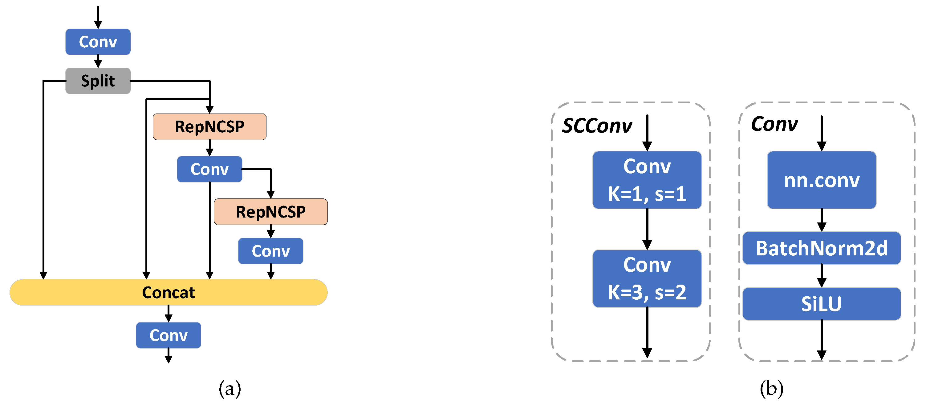
The backbone network is responsible for extracting features from input images, with traditional image classification networks commonly serving as the backbone. Leveraging the exceptional performance of YOLOv9 in object detection, we designed our backbone network using the GELAN structure proposed by YOLOv9, as shown in Figure 2. Specifically, it combines the CSPNet structure of YOLOv5’s backbone network with the ELAN of YOLOv7’s backbone network. This generalizes the functionality of ELAN, which originally stacked only convolutional layers, into a new architecture that can utilize any type of block. By adopting a gradient path planning design, it balances lightweight design, inference speed, and accuracy. By adjusting the depth and width of the network, this paper proposes two models with different parameter sizes: MT-TPPNet and MT-TPPNet(s).

Furthermore, to reduce computational costs and inspired by YOLOv10 [13], modifications were made to the commonly used downsampling operations in the YOLO backbone network. In YOLO models, downsampling operations typically use standard 3 × 3 convolutions to perform both spatial downsampling and channel transformation simultaneously, which introduces significant computational overhead. We propose decoupling the spatial downsampling and channel transformation operations for more efficient downsampling. We use pointwise convolutions for channel transformation and then employ depthwise separable convolutions for spatial downsampling, as shown in Figure 2. This approach maximizes the retention of information during downsampling while reducing computational costs. These enhancements make our backbone more efficient than previous YOLO series models for such tasks.

2.1.2. APEX Mechanism

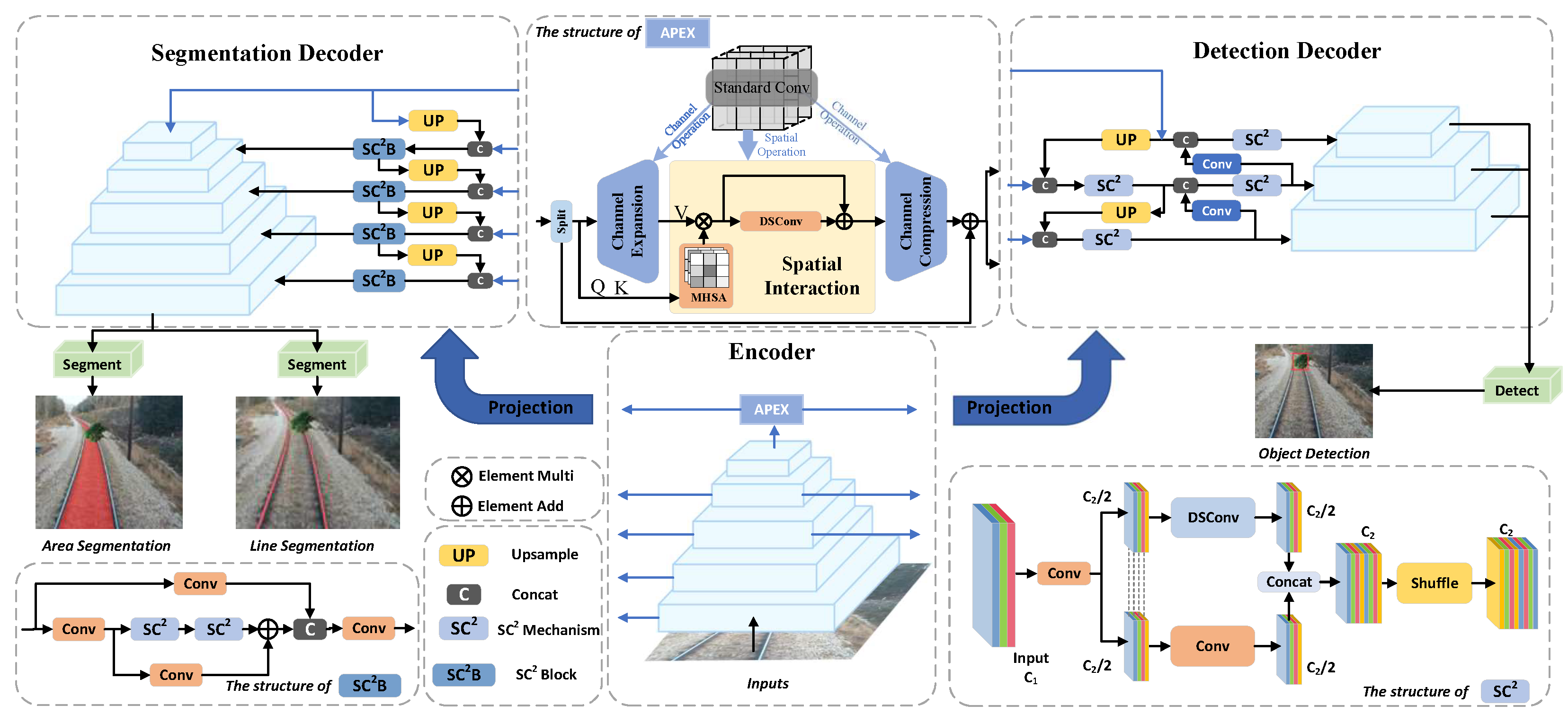
We revisit the processing pipeline of spatial and channel dimensions in conventional convolutions and decouple spatial interactions from channel mixing. As shown in Figure 3, the channel dimension is handled at both ends with $1\times 1$ convolutions for channel expansion/compression and mixing. The formula is:

$$\begin{array}{c}\hfill \widehat{F}=Con{v}_{1\times 1}\left(F\right)\in {\mathbb{R}}^{\lambda C\times H\times W}\end{array}$$

(1)

where F represents the input feature, $\lambda$ is the expansion rate. This decoupling ensures that the channel mixing and spatial interactions are not computationally coupled, which is a crucial advantage, particularly when dealing with high-dimensional features. By using $1\times 1$ convolutions, the method efficiently manages the complexity of the channel dimension without imposing excessive computational overhead.

In the middle of the pipeline, depthwise-separable convolution (DSConv) and Multi-Head Self-Attention (MHSA) [21,22,23,24] operate in parallel, offering a dual approach to modeling spatial interactions. The depthwise-separable convolution focuses on learning local spatial dependencies, while the MHSA, operating in the attention branch, captures long-range spatial dependencies by performing a global interaction across the feature map.

This parallelization of spatial interactions allows each mechanism to specialize in what it does best; DSConv efficiently captures local interactions with minimal computation, while MHSA effectively captures global relationships by leveraging attention weights. The interaction between these two mechanisms is facilitated through a gated fusion, where the features from both branches are combined, resulting in a more expressive representation of spatial information.

In the attention branch, we project the expanded high-dimensional representation to V, while the lower-dimensional representation is mapped to Q and K, yielding an asymmetric projection. The formula is:

$$\begin{array}{c}\hfill Q_i={\varphi }_{Q_i}\left(F\right)K_i={\varphi }_{K_i}\left(F\right)V_i^{ex}={\varphi }_{V_i^{ex}}\left(\widehat{F}\right)\end{array}$$

(2)

where $\varphi$ represents the projection operator. The process of spatial interaction can be expressed as follows:

$$\begin{array}{c}\hfill F_{ex}=\mathrm{MHSA}(Q,K,V^{ex})\end{array}$$

(3)

$$\begin{array}{c}\hfill F_s=\mathrm{DSConv}\left(F_{ex}\right)\oplus F_{ex}\end{array}$$

(4)

where $F_{ex}$ represents the features processed by the asymmetric projection MHSA. To further control computational cost, we partition the feature map along the channel dimension into two subsets; one subset is processed by the APEX mechanism to update the attention weights, whereas the other bypasses attention and is concatenated back afterward. This strategy significantly reduces the computational cost compared to standard attention mechanisms, which apply attention to the entire feature.

2.2. Decoder

2.2.1. ${\mathrm{SC}}^2$ Mechanism

As shown in Figure 3, the proposed ${\mathrm{SC}}^2$ mechanism can be formalized as follows. Given an input feature $X\in {\mathbb{R}}^{C\times H\times W}$, we construct two parallel convolutional branches. The first is a standard convolution branch:

$$\begin{array}{c}\hfill Y_{low}=\varphi \left(Conv\left(X\right)\right)\end{array}$$

(5)

The second is a depthwise-separable branch:

$$\begin{array}{c}\hfill Y_{high}=\varphi \left(DSConv\left(X\right)\right)\end{array}$$

(6)

where $\varphi (·)$ denotes batch normalization followed by a non-linear activation, $Conv(·)$ is a standard $k\times k$ convolution, $DSConv(·)$ is a depthwise-separable Convolution. The overall ${\mathrm{SC}}^2$ operator is then defined as:

$$\begin{array}{c}\hfill Y_{out}=\mathrm{Shuffle}\left([Y_{low},Y_{high}]\right)\end{array}$$

(7)

where $[·,·]$ denotes channel-wise concatenation and $\mathrm{Shuffle}(·)$ is the channel shuffle operation.

From the perspective of the frequency domain, the structure of ${\mathrm{SC}}^2$ can be viewed as a processing and modulation of input features across different frequency bands. Specifically, the standard convolution branch $Y_{low}$ tends to focus on low-frequency information, which allows it to model the channel dimension and capture semantic information within the image. On the other hand, the depthwise–separable branch $Y_{high}$ effectively severs inter-channel dependencies and emphasizes local details and high-frequency components such as edges, textures, and fine structures. By paralleling these two branches and mixing them through the shuffle operation, ${\mathrm{SC}}^2$ enables the network to better balance high-frequency spatial details and low-frequency semantic associations when processing multi-scale image features, while simultaneously reducing computational overhead.

2.2.2. Head

The decoder processes feature maps from the neck and generates predictions for each task, such as object classification, bounding boxes, and masks for segmented objects. In our approach, we utilize two distinct heads: a detection head and a segmentation head.

The detection head employs a decoupled method similar to YOLOv8, utilizing convolutional layers to convert high-dimensional features into class predictions and bounding boxes, without the need for an object branch, making it an anchor-free detector. During validation and prediction, the input passes through three different resolutions, and the output is a tensor containing both class and bounding box predictions. In training mode, the detection head uses convolutional layers on each input to generate three tensors, each with class predictions and bounding boxes corresponding to its resolution. These tensors are then used to compute the loss function.

The segmentation head is consistent for different segmentation tasks. It consists of several convolutional layers to capture contextual information, followed by a deconvolutional layer that restores the resolution to match the original image. Finally, a pixel-level binary mask is generated, with 0 representing the background and 1 representing the object, matching the size of the original image.

2.3. Loss Function

We adopt an end-to-end training approach and a multi-task loss function. Specifically, our loss function comprises three components: one for detection and two for segmentation. The formula is shown as follows:

$$Loss=Los{s}_{\det }+Los{s}_{\mathrm{segda}}+Los{s}_{\mathrm{segll}}$$

(8)

where $Los{s}_{\det }$ for the object detection task, $Los{s}_{\mathrm{segda}}$ for the drivable area segmentation task, and $Los{s}_{\mathrm{segll}}$ for the lane line segmentation task.

For the detection task, the loss function consists of two main components: the classification branch and the bounding box branch. The classification branch uses binary cross-entropy loss, denoted as ${Loss}_{CE}$. The bounding box branch incorporates Distribution Focal Loss (DFL) [25], denoted as ${Loss}_{DFL}$, and Complete Intersection over Union (CIoU) [26], denoted as ${Loss}_{CIoU}$. As a result, the detection loss function ${Loss}_{\det }$ is defined as follows:

$${Loss}_{det}={{\lambda }_{DFL}Loss}_{DFL}+{\lambda }_{CIoU}{Loss}_{CIoU}{+\lambda }_{CE}{Loss}_{CE}$$

(9)

where ${\lambda }_{DFL}$, ${\lambda }_{CIoU}$, ${\lambda }_{CE}$ are corresponding coefficients.

$$\begin{array}{cc}\hfill & {Loss}_{DFL}\left(S_i,S_{i+1}\right)=\hfill \\ \hfill & -(\left(y_{i+1}-y\right)log\left(S_i\right)+\left(y-y_i\right)log\left(S_{i+1}\right))\hfill \end{array}$$

(10)

where $S_i={\displaystyle \frac{y_{i+1}-y}{y_{i+1}-y_i}}$, $S_{i+1}={\displaystyle \frac{y_i-y}{y_i-y_{i+1}}}$. y represents the true values of the bounding box coordinates, expressed as decimals. $y_{i+1}$ is ceiling of ground truth y. $y_i$ is floor of ground truth y. ${Loss}_{DFL}$ measures the displacement between the predicted and ground truth feature locations, aiming to bring the predicted bounding box closer to the actual bounding box.

$${Loss}_{CIoU}=1-IoU+{\displaystyle \frac{{\rho }^2\left(b,b^{gt}\right)}{c^2}}+\alpha v$$

(11)

$$\alpha ={\displaystyle \frac{v}{\left(1-IoU\right)+v}}$$

(12)

$$v={\displaystyle \frac{4}{{\pi }^2}}{\left(arctan{\displaystyle \frac{{\omega }_{gt}}{h_{gt}}}-arctan{\displaystyle \frac{\omega }{h}}\right)}^2$$

(13)

$$CIoU=IoU-({\displaystyle \frac{{\rho }^2\left(b,b^{gt}\right)}{c^2}}+\alpha v)$$

(14)

where b denotes the center of the predicted box, and $b^{gt}$ represents the center of the ground truth box. $\rho$ is the Euclidean distance between the predicted point and the ground truth point. c refers to the diagonal length of the smallest enclosing rectangle between the two boxes. v and $\alpha$ are coefficients that control the ratio. h denotes the width and height of the predicted box, while ${\omega }_{gt}$ and $h_{gt}$ represent the width and height of the ground truth box. ${Loss}_{CIoU}$ combines factors like overlap, distance, and aspect ratio consistency to measure the difference between the predicted and ground truth bounding boxes. As a result, it allows the model to more precisely locate the object’s shape, size, and orientation.

$${Loss}_{CE}=-[y_{n}log{x}_n+\left(1-y_n\right)log(1-x_n)]$$

(15)

where $x_n$ represents the predicted classification for each object, and $y_n$ is the ground truth for each object. ${Loss}_{CE}$ quantifies the classification error between the predicted and ground truth values.

For the segmentation task, we use the same loss function. That is, the formulations of ${Loss}_{segda}$ and ${Loss}_{segll}$ are identical. We collectively refer to them as ${Loss}_{seg}$. The formula is as follows:

$${Loss}_{seg}={{\lambda }_{FL}Loss}_{FL}+{\lambda }_{TL}{Loss}_{TL}$$

(16)

where $Los{s}_{FL}$ and ${Loss}_{TL}$ are the Focal loss [27] and Tversky loss [28], respectively. Both are widely used loss functions in segmentation tasks. ${\lambda }_{FL}$ and ${\lambda }_{TL}$ are the corresponding weight coefficients.

$${Loss}_{FL}=-{\alpha }_t{\left(1-p_t\right)}^{\gamma }log\left(p_t\right)$$

(17)

where ${\left(1-p_t\right)}^{\gamma }$ is the modulation factor, $\gamma$ is the adjustable focusing parameter, and ${\alpha }_t$ is the class weighting factor, used to address class imbalance. $p_t$ represents the predicted probability for each class.

Focal loss provides a powerful solution for handling imbalanced samples, ensuring that the model does not become overly biased toward the dominant and easy-to-learn classes. Instead, it places more emphasis on the challenging and underrepresented areas.

$${Loss}_{TL}=1-{\displaystyle \frac{TP}{TP+\alpha FN+\beta FP}}$$

(18)

Tversky loss is an extension of Dice loss, incorporating two additional parameters ($\alpha$ and $\beta$) to assign distinct weights to false positives and false negatives, thereby improving its ability to address imbalanced tasks.

2.4. Training

Our training approach differs from the popular training methods used in other multi-task networks, such as those in autonomous driving tasks. We adopt an end-to-end training mode, where backpropagation is performed only once per batch. This means the entire network is optimized collectively, without freezing specific layers or alternating optimizations, thus reducing training time. In each epoch, the required predictions $\widehat{y}$, including information such as detection bounding boxes, classification, and segmentation masks, are obtained through a single forward pass. Subsequently, the loss for each task is calculated and summed to form a single loss, Loss. Then, backward propagation is executed only once to optimize the model for all tasks. After completing a training phase, the model is evaluated. If there is no improvement in performance compared to the last 50 epochs, training is terminated early. Otherwise, training will stop after 300 epochs.

3. Experiments and Results

3.1. Experiment Details

3.1.1. Datasets

The proposed model is evaluated using two datasets: (1) Multi-RID datasets consist of 3500 images of railway scenes. These images were collected in the field using the HIKROBOT MV-CA013-A0GC industrial camera (HIKROBOT, Hangzhou, China). Considering the rapid development of diffusion models, we supplemented the dataset by generating additional railway scene images using the state-of-the-art generative model SDXL [29]. Furthermore, a subset of railway scene images from open-source datasets [4] was selected to further augment the dataset. All multi-task labels were manually annotated by our team, and the intrusion object detection task includes seven common categories: person, stone, car, bike, train, animal, and tree. (2) BDD 100K datasets originating from the Berkeley DeepDrive Laboratory, is a crucial resource for autonomous driving research. It contains 100,000 samples with multi-task annotations.

3.1.2. Evaluation Metrics

For the object detection task, we use recall and mAP50 as evaluation metrics, both of which are widely used in detection tasks. Recall measures the model’s ability to correctly detect all object instances of a given class, while mAP50 is calculated by averaging the precision across all categories with an Intersection over Union (IoU) threshold of 0.5. Notably, average precision (AP) represents the area under the precision-recall curve.

For the segmentation task, similar to YOLOP, we use mIoU to assess the drivable area segmentation. For the track line segmentation task, we use accuracy and IoU as evaluation metrics. However, due to the imbalance in pixel numbers between background and foreground in track line segmentation, we use balanced accuracy, a more meaningful metric. Traditional accuracy tends to favor classes with larger sample sizes, leading to biased results, whereas balanced accuracy ensures a fairer evaluation by considering the precision of each class.

$$mIoU={\displaystyle \frac{1}{N}}\sum _{i=1}^{N}Io{U}_i$$

(19)

$$IoU={\displaystyle \frac{TP}{TP+FP+FN}}$$

(20)

$$BalancedAccuracy={\displaystyle \frac{TPR+TNR}{2}}$$

(21)

where N is the number of categories, $TPR={\displaystyle \frac{TP}{TP+FN}}$, and $TNR={\displaystyle \frac{TN}{TN+FP}}$.

3.2. Experiment Results

In this section, we train our model end-to-end on both the BDD 100K and our self-built dataset and then compare it with other outstanding methods on all three tasks.

3.2.1. Inference Speed

One of the primary challenges in deep learning applications is inference speed, which is particularly critical in the context of railway intrusion detection. In

Table 1. Comparison of different models in terms of parameters and FPS.

Model	Parameters	FPS (ba = 16)
YOLOv8s(seg)	11.79 M	256
YOLOv8s(det)	11.13 M	277
A-YOLOM(s) [18]	13.6 M	298
MT-TPPNet(s)	3.71 M	322
MT-TPPNet	13.83 M	285

, we present the FPS of several models, including our own, which were replicated and tested under identical conditions. To clearly highlight the performance differences, all FPS tests were conducted on a Tesla V100 GPU with a batch size of 16, thereby amplifying the FPS variations across the models. We excluded the preprocessing and postprocessing times. Additionally, we report the number of parameters for each model as part of the evaluation.

3.2.2. Multi-RID

As shown in

Table 2. Railway intrusion object detection results. ‘N/A’ indicates unpublished parameters or different evaluation metrics used. Bolded data indicates the best results.

Model	Intrusion Object Detection
	Parameters	Recall (%)	mAP50 (%)
YOLOv8s(det)	11.13 M	82.1	67.7
YOLOv8n(det)	3.01 M	80.9	66.3
YOLOv9(m) [11]	20.0 M	80.5	69.7
YOLOv10(m) [13]	16.49 M	82.5	71.6
MultiNet [20]	N/A	78.3	70.1
YOLOP [19]	7.9 M	80.6	69.7
A-YOLOM(n) [18]	4.43 M	82.4	65.0
A-YOLOM(s) [18]	13.61 M	78.4	69.4
MT-TPPNet(s)	3.71 M	81.8	70.2
MT-TPPNet	13.83 M	83.7	72.4

and

Table 3. Railway area and rail-track line segmentation results. ‘N/A’ indicates unpublished parameters or different evaluation metrics used. Bolded data indicates the best results.

Model	Area	Track-Line
	mIoU (%)	Accuracy (%)	IoU (%)
YOLOv8s(seg)	92.7	87.5	58.2
SCNN [16]	N/A	N/A	62.1
PSPNet [15]	90.6	N/A	N/A
YOLOP [19]	92.7	87.8	68.2
MultiNet [20]	91.1	N/A	N/A
A-YOLOM(n) [18]	92.4	88.4	67.4
A-YOLOM(s) [18]	92.9	88.2	68.0
MT-TPPNet(s)	93.1	88.7	68.1
MT-TPPNet	93.4	88.9	68.8

, the quantitative evaluation results demonstrate that MT-TPPNet achieves the highest mAP50 in the TPP task, surpassing the single-task YOLOv10 and the multitask model YOLOP by 0.8% and 2.7%, respectively. In terms of parameter count, although the complexity of MT-TPPNet(s) is comparable to that of YOLOv8n(det), it still improves recall and mAP. This indicates that our multitask learning approach allows different tasks to assist each other, further enhancing the performance of individual tasks.

In both segmentation tasks, MT-TPPNet also achieves state-of-the-art performance. In the area segmentation task, it surpasses YOLOP by 0.7% in mIoU, and in the rail track line segmentation task, it outperforms A-YOLOM by 0.7% in accuracy and 0.8% in IoU. Its unified architecture and shared loss function also eliminate the need for task-specific hyperparameter tuning.

3.2.3. BDD 100K

This section presents our method’s experimental results on the BDD 100K dataset. Similarly to the previous section, we compare our method with those specifically designed for each individual task.

Following YOLOP’s class-merging strategy, cars, buses, trucks, and trains are grouped into a single ‘vehicle’ category. As shown in

Table 4. Traffic object detection results; ‘N/A’ indicates unpublished parameters or different evaluation metrics used. Bolded data indicates the best results.

Model	Traffic Object Detection
	Parameters	Recall	mAP50
YOLOv8(n) (det)	3.01 M	82.2	75.1
YOLOv10(m) [13]	16.49 M	72.5	81.8
YOLOP [19]	7.9 M	88.6	76.5
MultiNet [20]	N/A	81.3	60.2
DLT-Net [30]	N/A	89.3	68.4
A-YOLOM(n) [18]	4.43 M	85.3	78.0
A-YOLOM(s) [18]	13.61 M	86.9	81.1
MT-TPPNet(s)	3.71 M	83.1	76.8
MT-TPPNet	13.83 M	89.4	83.2

and

Table 5. Drivable area and lane line segmentation results; ‘N/A’ indicates unpublished parameters or different evaluation metrics used. Bolded data indicates the best results.

Model	Area	Lane Line
	mIoU	Accuracy (%)	IoU (%)
SCNN [16]	N/A	N/A	15.84
YOLOv8n(seg)	78.1	80.5	22.9
PSPNet [15]	89.6	N/A	N/A
MultiNet [20]	71.6	N/A	N/A
A-YOLOM(n) [18]	90.5	81.3	28.2
A-YOLOM(s) [18]	91.0	84.9	28.8
YOLOP [19]	91.2	84.2	26.5
MT-TPPNet(s)	89.8	84.8	28.8
MT-TPPNet	91.6	85.1	28.9

, MT-TPPNet attains the highest mAP50, outperforming A-YOLOM(s) and YOLOP by 2.1% and 6.7%, respectively, and surpassing all YOLO baselines. These results demonstrate the strong cross-task transfer capability of our model. Table 5 presents the quantitative results for both the drivable area and lane line segmentation tasks.

For drivable-area segmentation, MT-TPPNet surpasses YOLOP and A-YOLOM in terms of mIoU by 0.4% and 0.6%, respectively. Although MT-TPPNet(s) attains a slightly lower mIoU than YOLOP, it still outperforms methods such as YOLOv8 and PSPNet, while maintaining a considerably smaller parameter budget. For the lane line segmentation task, MT-TPPNet likewise achieves the best performance in terms of IoU. Specifically, MT-TPPNet exceeds A-YOLOM(s) by 0.1%, while MT-TPPNet(s) surpasses YOLOP by 2.3%. Moreover, our models outperform other baselines, including YOLOv8n (seg), MultiNet, and PSPNet. These results underscore the strong cross-task transferability of our approach.

3.2.4. Visualization

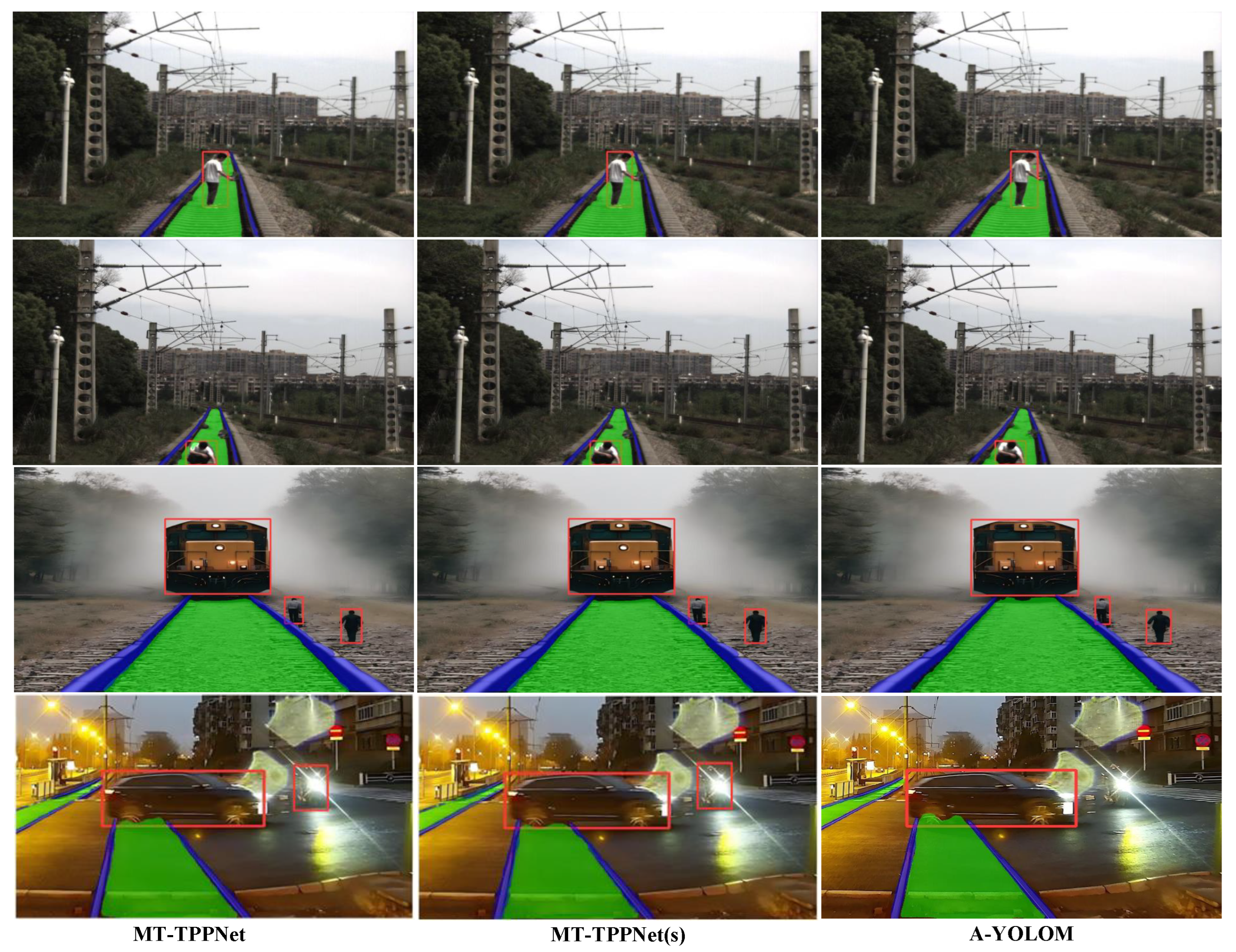
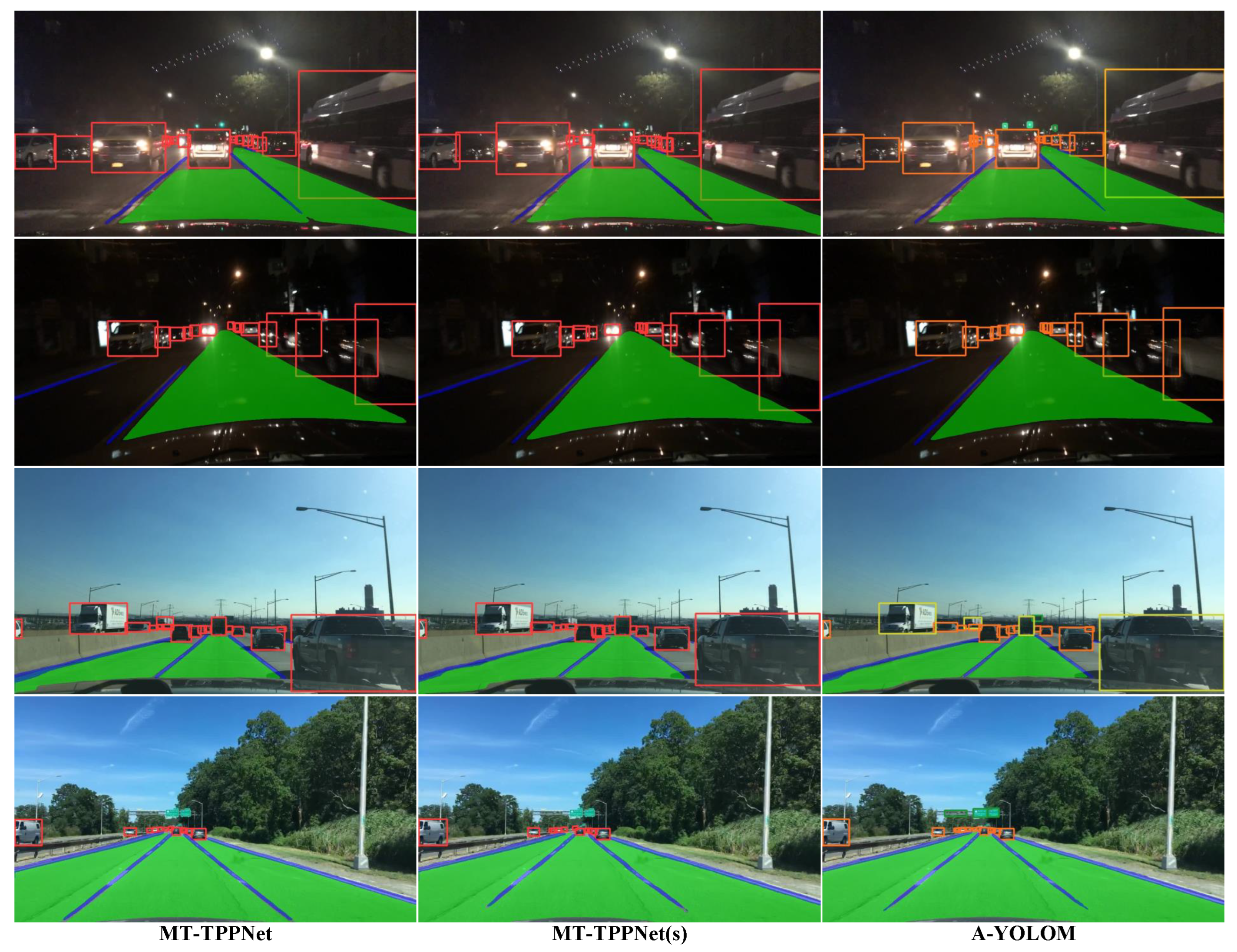
This section evaluates our model on railway intrusion detection and autonomous driving tasks under sunlight, night, rain, and snow. Figure 4 shows precise detection with smooth boundary and railway line annotations on the railway dataset. Figure 5 demonstrates performance comparable to A-YOLOM on BDD 100K in both day and night, effectively identifying vehicles, lanes, and drivable areas. The only shortcoming is slightly less smooth drivable area edges, yet the results confirm the model’s versatility for railway intrusion and broader multi-task applications.

Figure 5 displays the visual results of our model on the BDD 100K dataset. We compare our model with A-YOLOM, an outstanding work in the field of autonomous driving. As shown, our model performs similarly to A-YOLOM(s) in both daytime and nighttime conditions. It effectively detects vehicles and clearly displays lane markings and driving areas. The only noticeable difference is in the smoothness of the boundaries at the edges of the driving area, where our model’s performance is slightly weaker. This visual result highlights that our model is not only capable of effectively handling railway foreign object intrusion detection tasks but is also adaptable to other multi-task scenarios as needed.

3.3. Ablation Studies

This section reports the ablation experiments conducted on the Multi-RID dataset, aimed at quantifying the contribution of each component in MT-TPPNet, as shown in

Table 6. The ablation study for the APEX and SC², ‘Acc’ represents the balanced accuracy. Bolded data indicates the best results.

Model	APEX	${\mathrm{SC}}^2$	Parameters	Recall (%)	mAP50 (%)	mIoU (%)	Acc (%)	IoU (%)
MT-TPPNet(s)	-	-	3.55 M	78.1	67.6	92.1	87.7	67.2
	✓	-	3.87 M	79.6	68.3	92.6	88.2	67.9
	-	✓	3.39 M	78.4	67.8	92.2	88.2	67.7
	✓	✓	3.71 M	81.8	70.2	93.1	88.7	68.1
MT-TPPNet	-	-	13.27 M	82.5	71.1	92.6	88.1	67.7
	✓	-	14.53 M	83.6	72.3	93.2	88.8	68.6
	-	✓	12.57 M	83.0	71.9	93.1	88.2	68.1
	✓	✓	13.83 M	83.7	72.4	93.4	88.9	68.8

. Compared to the baseline model, the introduction of the APEX mechanism in the encoder results in improvements across various metrics, including a 1.2% increase in mAP50, a 0.6% increase in mIoU, and a 0.9% increase in IoU. These results demonstrate that the APEX mechanism can enhance the performance of different sub-tasks simultaneously. After incorporating the ${\mathrm{SC}}^2$ mechanism into the decoder, the model shows a 0.8% improvement in mAP50 and a 0.5% improvement in mIoU. Notably, the overall number of model parameters decreases to some extent, indicating that the introduction of the ${\mathrm{SC}}^2$ mechanism not only slightly improves model performance but also reduces computational cost.

4. Conclusions

This study presents an end-to-end lightweight multi-task model for the TPP task. To enhance the performance and generalization ability of all sub-tasks, we introduce the APEX mechanism by rethinking and decoupling the conventional convolution process along the spatial and channel dimensions. This decoupling enables APEX to exploit attention mechanisms with complementary inductive biases, thereby jointly and effectively improving the performance of the three sub-tasks. In addition, the decoder built upon the ${\mathrm{SC}}^2$ mechanism not only further boosts overall performance but also reduces the number of model parameters, thus satisfying real-time processing requirements. Extensive qualitative and quantitative experiments on our self-built Multi-RID dataset and the public BDD 100K dataset demonstrate that, on the challenging TPP task, the proposed model achieves state-of-the-art performance across all sub-tasks. In future work, we plan to incorporate additional traffic-scene sub-tasks into the framework and further optimize the model for deployment on edge devices.

References

1. Gašparík, J.; Bulková, Z.; Dedík, M. Prediction of Transport Performance Development Due to the Impact of COVID-19 Measures in the Context of Sustainable Mobility in Railway Passenger Transport in the Slovak Republic. Sustainability 2024, 16, 5283. [Google Scholar] [CrossRef]
2. Stopka, O.; Stopková, M.; Ližbetin, J.; Soviar, J.; Caban, J. Development Trends of Electric Vehicles in the Context of Road Passenger and Freight Transport. In Proceedings of the International Science-Technical Conference Automotive Safety, Kielce, Poland, 21–23 October 2020. [Google Scholar]
3. Qiao, W.; Wang, J.; Lu, D.; Liu, J.; Cai, B. BDS for Railway Train Localization Test and Evaluation Using 3D Environmental Characteristics. In Proceedings of the International Conference on Electromagnetics in Advanced Applications, Lisbon, Portugal, 2–6 September 2024. [Google Scholar]
4. Cao, Z.W.; Qin, Y.; Jia, L.M.; Xie, Z.Y.; Gao, Y.; Wang, Y.G. Railway Intrusion Detection Based on Machine Vision: A Survey, Challenges, and Perspectives. IEEE Trans. Intell. Transp. Syst. 2024, 25, 6427–6448. [Google Scholar] [CrossRef]
5. Cao, Z.W.; Qin, Y.; Jia, L.M.; Xie, Z.Y.; Gao, Y.; Wang, Y.G. A systematic review of the literature on safety measures to prevent railway suicides and trespassing accidents. Accident. Anal. Prev. 2015, 81, 30–50. [Google Scholar]
6. Havârneanu, G.M.; Bonneau, M.H.; Colliard, J. Lessons learned from the collaborative European project RESTRAIL: REduction of suicides and trespasses on RAILway property. Eur. Transp. Rer. Rev. 2016, 8, 16. [Google Scholar] [CrossRef]
7. Wang, X.; Liu, J.; Khattak, A.J.; Clarke, D. Non-crossing rail-trespassing crashes in the past decade: A spatial approach to analyzing injury severity. Safety. Sci. 2016, 82, 44–45. [Google Scholar] [CrossRef]
8. Li, H.L.; Li, J.; Wei, H.B.; Liu, Z.; Zhan, Z.F.; Ren, Q.L. Slim-neck by GSConv: A lightweight-design for real-time detector architectures. J. Real-Time Image Pr. 2024, 21, 62. [Google Scholar] [CrossRef]
9. Zhang, J.N.; Li, X.T.; Li, J.; Liang, L. Rethinking Mobile Block for Efficient Attention-based Models. In Proceedings of the IEEE/CVF International Conference on Computer Vision, Paris, France, 1–6 October 2023. [Google Scholar]
10. Ren, S.Q.; He, K.M.; Girshick, R.; Sun, J. Faster R-CNN: Towards Real-Time Object Detection with Region Proposal Networks. IEEE Trans. Pattern Anal. Mach. Intell. 2024, 39, 1137–1149. [Google Scholar] [CrossRef]
11. Wang, C.Y.; Yeh, I.H.; Liao, H.Y.M. YOLOv9: Learning What You Want to Learn Using Programmable Gradient Information. In Proceedings of the European Conference on Computer Vision, Milan, Italy, 29 September–4 October 2024. [Google Scholar]
12. Wang, C.Y.; Bochkovskiy, A.; Liao, H.Y.M. YOLOv7: Trainable Bag-of-Freebies Sets New State-of-the-Art for Real-Time Object Detectors. In Proceedings of the IEEE/CVF Conference on Computer Vision and Pattern Recognition, Vancouver, BC, Canada, 18–20 June 2023. [Google Scholar]
13. Wang, A.; Chen, H.; Liu, L.H.; Chen, K.; Lin, Z.J.; Han, J.G.; Din, G.G. YOLOv10: Real-Time End-to-End Object Detection. In Proceedings of the International Conference on Neural Information Processing Systems, Vancouver, BC, Canada, 10–15 December 2024. [Google Scholar]
14. Paszke, A.; Chaurasia, A.; Kim, S.; Culurciello, E. Enet: A deep neural network architecture for real-time semantic segmentation. arXiv 2016, arXiv:1606.02147. [Google Scholar] [CrossRef]
15. Zhao, H.S.; Shi, J.P.; Qi, X.J.; Wang, X.G.; Jia, J.Y. Pyramid Scene Parsing Network. In Proceedings of the IEEE/CVF Conference on Computer Vision and Pattern Recognition, Honolulu, HI, USA, 21–26 July 2017. [Google Scholar]
16. Pan, X.G.; Shi, J.P.; Luo, P.; Wang, X.G.; Tang, X.O. Spatial as Deep: Spatial CNN for Traffic Scene Understanding. In Proceedings of the AAAI Conference on Artificial Intelligence, New Orleans, LA, USA, 2–7 February 2018. [Google Scholar]
17. Hou, Y.N.; Ma, Z.; Liu, C.X.; Loy, C.C. Learning Lightweight Lane Detection CNNs by Self Attention Distillation. In Proceedings of the IEEE/CVF International Conference on Computer Vision, Seoul, Republic of Korea, 27 October–2 November 2019. [Google Scholar]
18. Wang, J.Y.; Wu, Q.M.J.; Zhang, N. You Only Look at Once for Real-Time and Generic Multi-Task. IEEE Trans. Veh. Technol. 2024, 73, 12625–12637. [Google Scholar] [CrossRef]
19. Wu, D.; Liao, M.W.; Zhang, W.T.; Wang, X.G. Yolop: You only look once for panoptic driving perception. Mach. Intell. Res. 2022, 19, 550–562. [Google Scholar] [CrossRef]
20. Teichmann, M.; Weber, M.; Zöllner, M.; Cipolla, R.; Urtasun, R. MultiNet: Real-time Joint Semantic Reasoning for Autonomous Driving. In Proceedings of the IEEE Intelligent Vehicles Symposium, New York, NY, USA, 26–30 June 2018. [Google Scholar]
21. Zhang, Q.M.; Zhang, J.; Xu, Y.F.; Tao, D.C. Vision Transformer With Quadrangle Attention. IEEE Trans. Pattern Anal. Mach. Intell. 2024, 46, 3608–3624. [Google Scholar] [CrossRef] [PubMed]
22. Grainger, R.; Paniagua, T.; Song, X.; Cuntoor, N.; Lee, M.W.; Wu, T.F. PaCa-ViT: Learning Patch-to-Cluster Attention in Vision Transformers. In Proceedings of the IEEE/CVF Conference on Computer Vision and Pattern Recognition, Vancouver, BC, Canada, 18–22 June 2023. [Google Scholar]
23. Zhu, L.; Wang, X.J.; Ke, Z.H.; Zhang, W.Y.; Lau, R. BiFormer: Vision Transformer with Bi-Level Routing Attention. In Proceedings of the IEEE/CVF Conference on Computer Vision and Pattern Recognition, Vancouver, BC, Canada, 18–22 June 2023. [Google Scholar]
24. Vaswani, A.; Shazeer, N.; Parmar, N.; Uszkoreit, J.; Jones, L.; Gomez, A.N.; Kaiser, Ł.; Polosukhin, I. Attention is all you need. In Proceedings of the International Conference on Neural Information Processing Systems, San Diego, CA, USA, 4–9 December 2017. [Google Scholar]
25. Li, X.; Wang, W.H.; Wu, L.J.; Chen, S.; Hu, X.L.; Li, J.; Tang, J.H.; Yang, J. Generalized focal loss: Learning qualified and distributed bounding boxes for dense object detection. In Proceedings of the International Conference on Neural Information Processing Systems, Vancouver, BC, Canada, 6–12 December 2020. [Google Scholar]
26. Zheng, Z.H.; Wang, P.; Liu, W.; Li, J.Z.; Ye, R.G.; Ren, D.W. Distance-IoU loss: Faster and better learning for bounding box regression. In Proceedings of the AAAI Conference on Artificial Intelligence, New York, NY, USA, 7–12 February 2020. [Google Scholar]
27. Lin, T.Y.; Goyal, P.; Girshick, R.; He, K.; Dollár, P. Focal Loss for Dense Object Detection. In Proceedings of the IEEE/CVF International Conference on Computer Vision, Venice, Italy, 22–29 October 2017. [Google Scholar]
28. Salehi, S.S.M.; Erdogmus, D.; Gholipour, A. Tversky Loss Function for Image Segmentation Using 3D Fully Convolutional Deep Networks. In Proceedings of the International Workshop on Machine Learning in Medical Imaging, Quebec, ON, Canada, 10 September 2017. [Google Scholar]
29. Podell, D.; English, Z.; Lacey, K.; Blattmann, A.; Dockhorn, T.; Müller, J.; Penna, J.; Rombach, R. SDXL: Improving Latent Diffusion Models for High-Resolution Image Synthesis. In Proceedings of the International Conference on Learning Representations, Vienna, Austria, 7–11 May 2024. [Google Scholar]
30. Qian, Y.Q.; Dolan, J.; Yang, M. DLT-Net: Joint Detection of Drivable Areas, Lane Lines, and Traffic Objects. IEEE T. Intell. Transp. 2019, 21, 4670–4679. [Google Scholar] [CrossRef]
Figure 1. Multi-task in traffic panoptic perception: object detection, drivable area segmentation, and line segmentation. (a) Input. (b) Output.
Computers 14 00536 g001
Figure 2. Part of the backbone network structure. (a) GELAN structure. (b) Comparison of spatial–channel separation Conv and standard Conv structures.
Computers 14 00536 g002
Figure 3. Overall network structure of MT-TPPNet.
Computers 14 00536 g003
Figure 4. Visual comparison of results on the Multi-RID.
Computers 14 00536 g004
Figure 5. Visual comparison of results on the BDD 100K.
Computers 14 00536 g005