Abstract
This article describes a novel method for the multi-step forecasting of PM2.5 time series based on weighted averages and polynomial interpolation. Multi-step prediction models enable decision makers to build an understanding of longer future terms than the one-step-ahead prediction models, allowing for more timely decision-making. As the cases for this study, hourly data from three environmental monitoring stations from Ilo City in Southern Peru were selected. The results show average RMSEs of between 1.60 and 9.40 ug/m3 and average MAPEs of between 17.69% and 28.91%. Comparing the results with those derived using the presently implemented benchmark models (such as LSTM, BiLSTM, GRU, BiGRU, and LSTM-ATT) in different prediction horizons, in the majority of environmental monitoring stations, the proposed model outperformed them by between 2.40% and 17.49% in terms of the average MAPE derived. It is concluded that the proposed model constitutes a good alternative for multi-step PM2.5 time series forecasting, presenting similar and superior results to the benchmark models. Aside from the good results, one of the main advantages of the proposed model is that it requires fewer data in comparison with the benchmark models.
1. Introduction
The global burden of disease associated with the exposure to air pollution causes millions of deaths and years of healthy life lost annually [1]. The burden of disease attributable to air pollution is estimated to be on par with other major global health risks, such as unhealthy diet and smoking [2,3]; air pollution is now recognized as the greatest environmental threat [4] to human health.
PM2.5 is one of the main pollutants [5,6,7], and it can accumulate in the respiratory system. It is associated with numerous negative effects on the health, such as increased respiratory diseases and decreased lung function. Thus, PM2.5 can cause premature death in people with heart [8] or lung disease [9,10] and can lead to non-fatal myocardial infarctions [11], irregular heartbeats [12], aggravated asthma [13,14], reduced lung function, and increased respiratory symptoms, such as irritation in the airways [15], cough, and difficulty breathing.
In this context, it is clear that there is a need to implement air quality monitoring stations and, from these, develop tools that allow for the analysis and prediction of the volumes of PM2.5 and other pollutants. According to the literature, numerous works have been found that address the topic of PM2.5 forecasting; however, most studies have addressed PM2.5 forecasting through the implementation of one-step-ahead forecasting. This means that the models predict only one value, which is not very useful if the prediction of more than one value is required; thus, in this context, multi-step forecasting models become important.
The proposed model is a novel and simple multi-step model for PM2.5 forecasting. It is inspired by weighted moving averages [16,17] and polynomial interpolation [18]; it uses data that are closer to the predicted values because these are more relevant [19], assuming that the near future is close to the near past. In this sense, the proposed model uses data from just two days (48 h) to predict 24, 48, and 72 h in the future; thus, it requires a small amount of data to produce similar and superior results to those made by the state-of-the-art techniques such as deep learning-based approaches, including long short-term memory (LSTM), bidirectional LSTM (BiLSTM), gated recurrent unit (GRU), bidirectional GRU (BiGRU), and LSTM with attention mechanism (LSTM-ATT).
The main contributions of this work are as follows:
- -
- A novel model for multi-step forecasting of PM2.5 time series;
- -
- A comparative analysis between proposal results and benchmark models based on deep learning;
- -
- A web application for PM2.5 time series forecasting.
Some of the limitations of this work lie in the type of forecasting model that is proposed here (a univariate model) and in the number of case studies which is limited to three monitoring stations located in Southern Peru.
2. Literature Review
2.1. Overview of Forecasting Models
Forecasting models for time series have evolved from statistical models to machine learning and deep learning models. Among the statistical models, one of the best-known models is ARIMA [20]. Machine learning-based models include the support vector machine (SVM) [21], nearest neighbors regression [22], and ensemble models such as random forests [23], gradient boosting [24], and Adaboost [25]. Deep learning models such as those based on recurrent neural networks include LSTM, GRU, BiLSTM, BiGRU, and RNNs with attention layers; finally, those based on Transformers [26,27] are gaining popularity.
2.2. One-Step-Related Works in PM2.5 Forecasting
Most of the related works have proposed and implemented LSTMs; among these, the research presented in [18,28,29,30,31,32,33] has included decomposition techniques, and others have combined LSTM with other techniques. In [30], the authors added a decomposition technique named Singular Spectrum Analysis (SSA). In [28,29], bidirectional LSTM (BiLSTM) and LSTM were used, respectively. In [31], LSTM was combined with convolutional neural networks (CNNs). In [33], a bidirectional LSTM model was combined with a CNN model. In [32], an LSTM was used with decomposition techniques such as CEEMDAN and FCM. Additionally, in [34,35], GRU was implemented with data augmentation and with Q-Learning, respectively.
Support vector regression (SVR) and random forest have been used in works such as [36,37,38]. The first uses SVR in a hybrid way with quantum particle swarm optimization (QPSO), while the second adds a decomposition technique named hybrid modified variational mode decomposition, and the last one uses a random forest model alone.
Furthermore, some related works, including [39,40,41,42,43], implemented different approaches to those cited before. In [39], a Hammerstein recurrent neural network was proposed; in [24], a decomposition ensemble learning model was used, based on the variation-mode decomposition approach and a whale-optimization algorithm (IWOA); in [42], an attention-based deep neural network was used; in [43], a multivariate deep belief network using PM2.5 and temperature data was implemented; in [40], a multiple model adaptive unscented Kalman filter was utilized.
2.3. Multi-Step-Model-Related Works in PM2.5 Forecasting
In [44,45], the authors proposed an extreme learning machine (ELM), which was used to obtain MAPEs between 5.11% and 37.23% for three-step forecasting and MAPEs between 5.12% and 22.2% for seven-step forecasting.
In [46], a hybrid CNN–LSTM model was used for a ten-step forecasting, obtaining MAPEs between 22.09% and 25.94%.
In [47], AdaBoost was proposed, obtaining MAPEs between 15.32% and 23.75% for three-step forecasting.
In [48], a support vector machine (SVM) was used for four-step predictions, obtaining RMSEs between 8.16 and 39.04 ug/m3.
In [49], a self-organizing memory neural network was implemented for 1-, 4-, 8-, and 12-day forecasting, obtaining MAPEs between 6.66% and 14.08%.
In [50], a feature-selection approach based on a genetic algorithm was used to implement an LSTM model for one- to six-step forecasting, obtaining MAEs between 3.592 and 6.684.
In [51], a BiLSTM was used for three-step forecasting, obtaining MAPEs between 27.33% and 40.73%.
In [52,53], a CNN was proposed for ten-step predictions and four-step predictions, obtaining MAPEs between 28.51% and 33.29%.
Finally, in [54], a point system for three-step forecasting was implemented, obtaining MAPEs between 7.53% and 16.18%.
According to the literature review for single and multi-step PM2.5 forecasting, most researchers have focused on machine learning and deep learning techniques; some researchers considered hybrid models, decomposition techniques, and data augmentation. Most researchers addressed the problem of PM2.5 forecasting in a single step. According to [55], decisions about air quality often need to be made more than 10 h in advance; according to the literature, the maximum number of steps used for PM2.5 forecasting was 10 steps ahead (10 h). This finding served as a motivation for this work, prompting the authors to propose a different multi-step forecasting proposal with a greater number of steps than those reported in the literature. It is important to highlight that, according to the literature, the term “steps” refers to the number of forecasted points.
The main differences between the related literature and the present study are summarized in Table 1.

Table 1.
Differences between related research and the present study.
3. Materials and Methods
3.1. Data Collection
The hourly data used for this work were downloaded from OEFA’s server (located at https://pifa.oefa.gob.pe/VigilanciaAmbiental/, accessed on 2 May 2023), and they span the period between 1 August 2020 and 30 April 2023. They correspond to three environmental monitoring stations (Pacocha, Bolognesi, and Pardo) located at Ilo city, Moquegua region, Southern Peru.
The downloaded data had several missing values, so the days that presented missing values were discarded. The available records for each station remaining after this process are shown in Table 2. Likewise, since the present study addresses a regression problem, according to the literature for statistical models, the dataset was split into the following two sets: the training set (80%) and the test (20%) set.

Table 2.
Data of environmental monitoring stations.
3.2. Selection of Days
The proposed model does not work with all the training data; it only works with the two historical days. For this selection, first, the correlations of the hours between the last 24 days of the training data of the three stations were analyzed separately. For this, the data were organized in a matrix manner, and the correlation matrix that is commonly used for feature selection [56] in classification tasks using machine learning and deep learning models was utilized. The respective correlation matrices for each monitoring station are shown in Figure 1, Figure 2 and Figure 3.
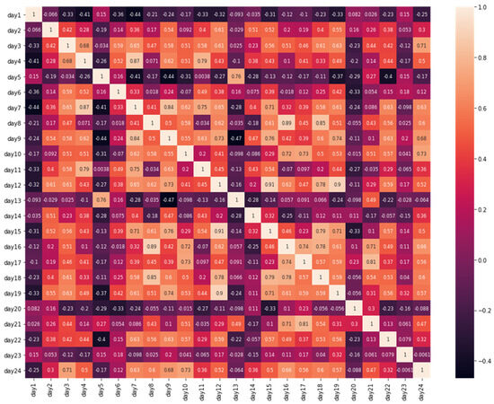
Figure 1.
The 20-day correlation of Pacocha station.
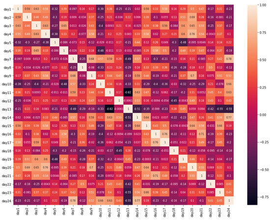
Figure 2.
The 20-day correlation of Bolognesi station.
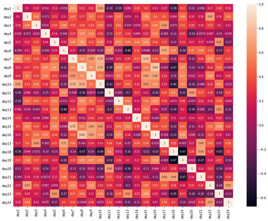
Figure 3.
The 20-day correlation of Pardo station.
In this study, the correlation between a given day and the subsequent days is of interest; this correlation can be determined by looking at the values above the main diagonal of the respective correlation matrix, C. If the day to be analyzed is located on the main diagonal in row i, then the prior days to i will begin in row i − 1, column j = i; thus, the average correlation is given by Equation (1). For the following previous day, it also starts in row i − 1 but in column j = i + 1 (2). The following previous day starts in row i − 1, column j = i + 2 (3), and so on.
Equations (1)–(3) can be summarized in (4) as follows:
where is the average correlation of day j.
Using Equation (4), Table 3 was formulated.

Table 3.
Average correlations between days.
According to Table 3, on day i, there is an average correlation of 0.2013 with the previous day, i − 1, an average correlation of 0.1527 with day i − 2, an average correlation of 0.2400 with day i − 3, and so on.
It is important to highlight that, according to Figure 4, the different numbers of days were used for estimating average correlations. Thus, for day i − 1, there are n − 1 days, for day i − 2, there are n − 2 days, and so on; for the last day, or the one furthest from the main diagonal, there is only one day.

Figure 4.
How matrix M is used to make predictions.
Just two days were chosen for the implementation of the proposed model. A greater number of days can be chosen, but the results do not improve significantly. According to Table 1, for the implementation of the proposed model, days 1 and 3 were chosen. Day 1 was chosen because—despite not having the highest average correlation—it showed a good correlation with the highest number of days (0.2013), with little deviation. It can be seen in all stations that there are correlations greater than 0.14. Similarly, day 3 was selected because it has an average correlation of 0.2400, which is higher than those of day 1, day 2, day 4, day 5, day 6, and others. Days 7 and 8 present average correlations higher than 0.22 and are higher than day 1, but they were discarded due to their deviation. For the Pacocha and Pardo stations, their correlations are higher than 0.30 and 0.20, respectively; for the Bolognesi station, the correlations are less than 0.10.
The result of this stage is a matrix, M, of the order 3 × 4, with the data of the last 72 h, according to Equation (5). The first row corresponds to day 3, the second to day 2, and the third to day 1. New rows (4th, 5th, 6th, …) are added according to the performed predictions.
Here, S is the training data vector of an environmental monitoring station and n is the vector length.
The first row contains the 24 h of day 3, the second contains the 24 h of day 2, and the third contains the 24 h of day 1.
According to Figure 4, in the first step, M was used to obtain the predicted day 1 (24 h ahead) using day 1 and day 3. Then, the predicted day 2 was obtained using day 2 and the predicted day 1. Finally, the predicted day 3 was obtained using day 1 and the predicted day 2. More details about the estimation of predicted days are presented in the next section.
3.3. Estimating Weighted Averages (WAs)
The hours of the two selected days in the previous stage were averaged; however, this was not performed in the traditional way, considering the same weight for each day. Instead, the values from Table 2 were used to create the matrix Corrs (6). The weights were important since the days did not have the same correlation.
The first row of the matrix represents the weights of days 1 and 3 for the Pacocha station, the second represents the weights of days 1 and 3 for the Bolognesi station, and the third represents the weights of days 1 and 3 for the Pardo station.
From (5), the weights for each station were obtained according to (7) as follows:
where i is the environmental monitoring station. According to (5), j is the day, 1 is the first day, and 2 is the third day. w1 is the weight for the first day and w3 is the weight for the third day.
According to Figure 4, in the predicted day 1, Sn−71 and Sn−23 were used for the first hour, Sn−70 and Sn−22 were used for the second hour, Sn−69 and Sn−21 were used for the third hour, and so on.
Then, the weighted average (WA) Equations (8)–(10) for different predicted days were implemented.
E1, E2, and E3 are the vectors of predicted days 1, 2, and 3, respectively. Equations (8)–(10) can be summarized in (11) as follows:
where i is the predicted day, j is the j-th hour of the day, w1 is the weight for day 1, and w3 is the weight for day 3.
An example of how WA (11) predicts 24 h for Pardo station can be seen in Figure 5.
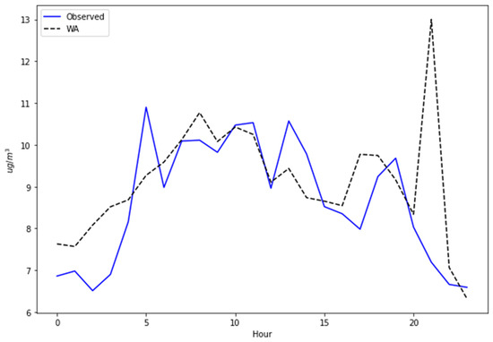
Figure 5.
The 24 predicted hours with the weighted average equation.
3.4. Applying Polynomial Interpolation (PI)
To reduce the error of the weighted average (WA) predictions, in this stage, polynomial interpolation (PI) was used to smooth the curve of the predicted values, bringing them closer to the observed ones.
For this, from the 24 predicted points in each iteration of WA, a representative number was selected; in this case, the optimal number was seven, being the seven positions, 0, 3, 7, 11, 15, 19, and 23. Then, NumPy’s polyfit function was used with the optimal degree of five. Finally, the obtained function was used to predict the 24 values. The corresponding polynomial function is expressed in Equation (12) as follows:
where a0, a1, a2, a3, a4, and a5 are the coefficients of the polynomial function.
Figure 6 shows a comparison between the observed values, the WA, and the WA + PI predicted values for 24 h for the Pacocha station.
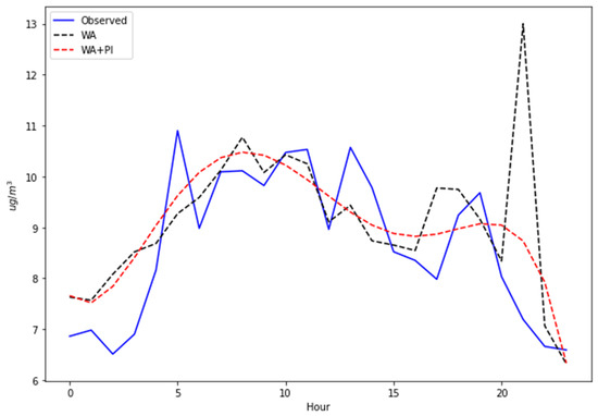
Figure 6.
Multi-step predictions of WA and WA + PI.
The corresponding algorithm for the WA + PI proposal is shown in Figure 7.
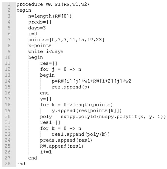
Figure 7.
The WA + PI algorithm.
According to Figure 7, the procedure receives RW, w1, and w2 as parameters. RW is a matrix with the data from the last three days of the training data. The algorithm was set to predict 3 days (72 h); for this, an iterative process (while) was performed, going from 0 to 2, predicting 24 h in each iteration. Between lines 12 and 16, the WA predictions were made. Between lines 17 and 20, from the WA predictions, the polynomial function was obtained using the array points. Between lines 21 and 25, the polynomial function was used to make predictions, and the RW matrix was updated. The process continued, with the next day being used to predict the following 24 h. The loop ended when 72 h had been predicted.
The corresponding obtained results are described in the Results and Discussion section.
3.5. Evaluation
The evaluation of the results was carried out through the root mean squared error (RMSE), which allows one to measure the error in terms of ug/m3, mean absolute percentage error (MAPE), which allows one to measure the error of the predictions in percentage terms, and finally the correlation coefficient R2, which allows one to measure the correlation between the predicted and observed values. These metrics are implemented through Equations (13)–(15) as follows:
where P is the predicted value vector, O is the observed value vector, is the mean of observed values, and is the mean of the predicted values.
4. Results and Discussion
In this section, the achieved results are described.
4.1. Results
4.1.1. Weighted Averages and Polynomial Interpolation (WA + PI)
Table 4, Table 5 and Table 6 show comparisons between WA and WA + PI for each environmental monitoring station.

Table 4.
Results of WA and WA + PI (Pacocha).

Table 5.
Results of WA and WA + PI (Bolognesi).

Table 6.
Results of WA and WA + PI (Pardo).
In Table 4, Table 5 and Table 6, it can be seen that, in terms of RMSE (66.67%) and MAPE (50.00%), in most cases, polynomial interpolation (PI) allows one to improve the results derived using the weighted average (WA), improving the WA between 0.0582% and 1.6433%; hence, one can see the importance of PI in the implementation of the model proposed in this work.
4.1.2. A Web Application Based on WA + PI
The constructed model was used for the implementation of a web application. It has a simple architecture, which includes the front-end and the back-end. HTML5, Javascript, Bootstrap, and Chart.js were used to implement the front-end. The back-end was Python, and the Flask framework was used for the development of the web application. Figure 8 shows the main view of the web application.
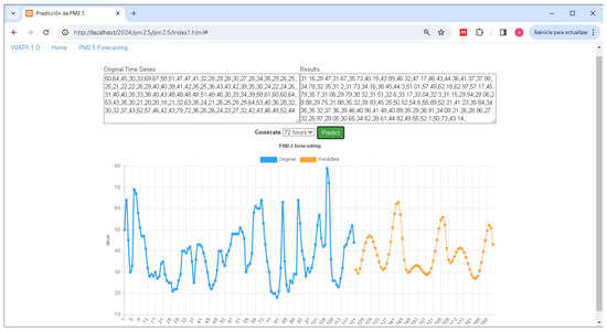
Figure 8.
Web application for PM2.5 forecasting.
4.2. Discussions
4.2.1. Comparison with Benchmark Models
To evaluate how the proposed model contributes to advancing the state of knowledge in this field, well-known, multi-step, deep learning-based, state-of-the-art models—such as LSTM, BiLSTM, GRU, BiGRU, and LSTM-ATT—were implemented.
LSTM is a type of recurrent neural network (RNN) that is used to process and predict data sequences. An LSTM cell is composed of an input gate, an output gate, and a forget gate, which enables useful information to be remembered.
The BiLSTM is based on LSTMs, with the main difference being that it is bidirectional. In LSTMs, information flows in a single direction from left to right; meanwhile, with BiLSTM, information flows in both directions, from left to right and from right to left. BiLSTMs can learn more complex relationships, but the computational cost is higher.
GRU is a type of RNN; GRU has fewer gates (only two: reset and update) and fewer parameters than LSTMs. LSTMs are more complex and effective in modeling complex patterns; meanwhile, GRU is more efficient and easier to train. The choice between an LSTM and a GRU depends on the specific problem and the available resources.
BiGRU is similar to BiLSTM, with the main difference being that the BiGRU is based on GRU.
LSTM-ATT is a variant of LSTMs that incorporates an attention mechanism to improve the ability to model data sequences. The attention mechanism allows the model to focus on certain parts of the input sequence that are more relevant to a specific task. This is useful when working with long sequences, where only some parts of the sequence are important for predictions.
A graphical view of the benchmark model architectures can be seen in Figure 9.
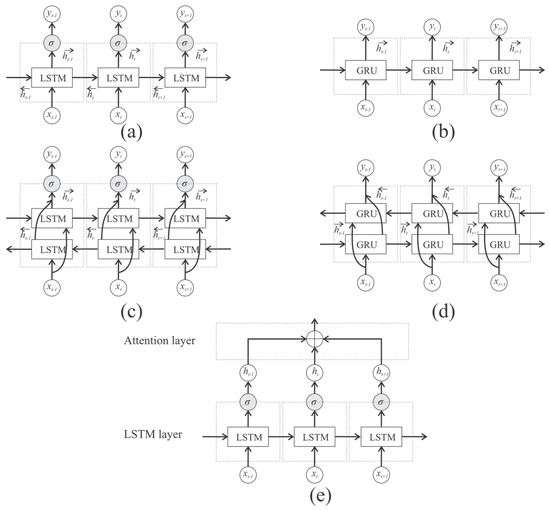
Figure 9.
Architectures of the benchmark models: (a) LSTM, (b) GRU, (c) BiLSTM, (d) BiGRU, and (e) LSTM−ATT.
The hyperparameters of the benchmark models are listed in Table 7.

Table 7.
Hyperparameters of the benchmark models.
The lock-back for each model was set to 24 h. RNNs, with no attention mechanism, include three layers of 30 neurons each, while RELU is the activation function, and drop_rates of 0.1 were used after each layer to avoid overfitting.
An LSTM with an attention mechanism includes one LSTM layer with 100 neurons, followed by a dense layer with one neuron and tanh as activation, an activation layer (softmax), a repeatVector(100), a permute layer, a multiply layer, a lambda, and a final dense layer with n neurons, depending on the number of hours to be predicted.
All models were trained with 100 epochs, using adam as the optimizer and mse as the loss function. The 100 epochs used produced the best results for each model.

Table 8.
The benchmark models vs. the proposed model in Pacocha station.

Table 9.
The benchmark models vs. the proposed model in Bolognesi station.

Table 10.
The benchmark models vs. the proposed model in Pardo station.
According to Table 8, for the Pacocha station, in terms of RMSE, the proposed model outperformed the benchmark models in most cases (66.67%) for 24 and 72 predicted hours, obtaining RMSEs of 4.0954 and 12.9212, respectively. For 48 predicted hours, the proposed model was only surpassed by the BiLSTM and LSTM. In terms of MAPE, the proposed model outperformed all the benchmark models (100%). In terms of R2, it outperformed all benchmark models for 24 predicted hours; it was outperformed by BiLSTM and BiGRU for 48 predicted hours; and for 72 predicted hours, it was outperformed by BiLSTM only.
According to Table 9, for the Bolognesi station, the proposed model obtained the worst results. In terms of RMSE, for the 24 predicted hours, the proposed model was the worst, with 3.2104 ug/m3; for the 48 predicted hours, the proposed model was outperformed by LSTM-ATT and LSTM. For the 72 predicted hours, the proposed model was the worst model, with 7.7738 ug/m3. In terms of MAPE, the proposed model was outperformed by all the benchmark models. In terms of R2, the proposed model was outperformed by all models for 24 and 48 predicted hours, and for 72 predicted hours, it outperformed only BiGRU. The best model for Bolognesi station was LSTM-ATT.
According to Table 10, for the Pardo station, the proposed model obtained the best results. In terms of RMSE and MAPE, the proposed model outperformed all the benchmark models. In terms of R2, for 24 predicted hours, the proposed model (0.6414) was outperformed by BiLSTM (0.6472); for 48 predicted hours, the proposed model (0.2315) was outperformed by BiLSTM (0.3075), LSTM (0.3008), and GRU (0.2422); for 72 predicted hours, the proposed model was outperformed by all the benchmark models except GRU.
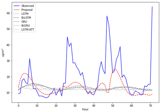
Figure 10.
The 72 predicted hours for Pacocha station.
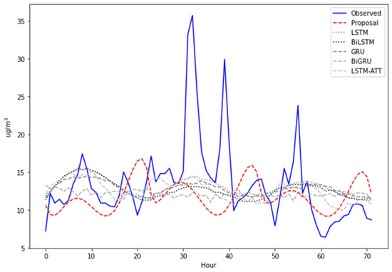
Figure 11.
The 72 predicted hours for Bolognesi station.

Figure 12.
The 72 predicted hours for Pardo station.
In this work, three different prediction horizons were experimented with for multi-step forecasting—24, 48, and 72 h. The proposed model produced similar and superior results to the benchmark models, surpassing them in most cases in terms of RMSE and MAPE. However, it is important to explain why the proposed model produced these results for the different environmental monitoring stations; for this purpose, correlations were determined between the first day of the test data and the last training days. Table 10 shows these correlations.
According to Table 11, it can be seen that in the case of the Bolognesi station—which is where the proposed model presented the worst results—the last training data that correspond to day 1 present a very low correlation (0.0115). Likewise, the data for the other day used, which is day 3, also present a very low correlation (−0.009).

Table 11.
Correlations between the first day of test data and the last training days.
However, for the Pacocha and Pardo stations, for the first day and third day, there are better correlations of between 0.293 and 0.6018, and this is reflected in the results of the proposed model.
The above means that the average correlation used for the selection of days may not be good in some cases; because it is an average, it may only be good for some cases. For future work, different day selections could be made for each station and not just the ones used in this work.
4.2.2. Comparison with Related Works
Next, the proposed model results were compared with the results of multi-step related works.
Finally, the results of the proposed model were compared with those reported in related works; according to Table 12, in terms of the five studies addressing MAPE, the research presented in [44,45,47,49,54] obtained MAPEs of 5.11%, 5.12%, 15.32%, 14.08%, and 7.53%. These studies reported MAPEs higher than those obtained by the proposed model (17.69%); three of them used three-step forecasting, and two of them used twelve- and seven-step forecasting. Therefore, there is an enormous difference between the number of steps in the related works and the proposed model. This is a factor that is in favor of the results presented in these other studies; this is because, as the number of steps increases, the accuracy of the results worsens.

Table 12.
Related works vs. proposal.
On the other hand, the results for the proposed model surpass the results presented in [46,51,53]; the authors of these works implemented techniques similar to the benchmark models implemented in the present paper.
In terms of RMSE, the proposed model considerably exceeds the RMSEs reported in [48,52].
5. Conclusions and Future Work
According to the obtained results, it can be concluded that the proposed model based on weighted averages (WAs) and polynomial interpolation (PI) constitutes a good alternative for the multi-step forecasting of PM2.5 time series. The proposed model outperformed the other models for most of the analyzed environmental monitoring stations. The well-known, state-of-the-art models that were used for these comparisons included LSTM, BiLSTM, GRU, BiGRU, and LSTM-ATT. The proposed model outperformed these models in terms of the average MAPE obtained (between 2.4010% and 17.6208%). One of the main advantages of the proposed model is that it requires few data compared to these benchmark models, which are based on deep learning.
Although the results are interesting, and the implemented benchmark models had been outperformed in most cases, some aspects still need improvement. The achieved MAPEs were between 17.69% and 28.91%. According to [57], if the MAPE is less than 10%, then the model is highly accurate; if the MAPE is between 10% and 20%, then the model is good; if the MAPE is between 20% and 50%, then the model is reasonable. Thus, the proposed model can be considered as being between good and reasonable; it should be highly accurate. In pursuit of a highly accurate rating, in future work, instead of working with only two days, it could be adjusted to function with three or more days, depending on the level of the correlations. Similarly, instead of polynomial interpolation, other types of interpolation, such as linear, Stineman, inverse distance weighting, or kriging, could be used. On the other hand, ensemble and hybrid models could be created with other forecasting techniques, such as autoregressive integrated moving average (ARIMA).
Author Contributions
Conceptualization, A.F. and H.T.-C.; Methodology, A.F.; Software, A.F.; Validation, V.Y.-M. and C.R.-C.; Formal analysis, A.E.-E.; Investigation, C.R.-C. and A.E.-E.; Resources, V.Y.-M.; Data curation, H.T.-C.; Writing—original draft, A.F.; Writing—review & editing, H.T.-C.; Visualization, A.E.-E.; Supervision, V.Y.-M.; Project administration, C.R.-C.; Funding acquisition, V.Y.-M. All authors have read and agreed to the published version of the manuscript.
Funding
This research received no external funding and the APC was funded by Universidad Nacional de Moquegua.
Data Availability Statement
Data are available at “https://pifa.oefa.gob.pe/VigilanciaAmbiental/ (accessed on 2 May 2023)” or by contact to the corresponding author.
Conflicts of Interest
The authors declare no conflict of interest.
References
- WHO. WHO Global Air Quality Guidelines. 2021. Available online: https://iris.who.int/bitstream/handle/10665/345329/9789240034228-eng.pdf?sequence=1&isAllowed=y (accessed on 5 July 2024).
- Martinez-Lacoba, R.; Pardo-Garcia, I.; Amo-Saus, E.; Escribano-Sotos, F. Socioeconomic, demographic and lifestyle-related factors associated with unhealthy diet: A cross-sectional study of university students. BMC Public Health 2018, 18, 1241. [Google Scholar] [CrossRef] [PubMed]
- Imanda, A.; Martini, S.; Artanti, K.D. Post hypertension and stroke: A case control study. Kesmas Natl. Public Health J. 2019, 13, 164–168. [Google Scholar] [CrossRef]
- Landrigan, P.J.; Stegeman, J.J.; Fleming, L.E.; Allemand, D.; Anderson, D.M.; Backer, L.C.; Brucker-Davis, F.; Chevalier, N.; Corra, L.; Czerucka, D.; et al. Human health and ocean pollution. Ann. Glob. Health 2020, 86, 151. [Google Scholar] [CrossRef]
- Abutalip, K.; Al-Lahham, A.; El Saddik, A. Digital Twin of Atmospheric Environment: Sensory Data Fusion for High-Resolution PM2.5 Estimation and Action Policies Recommendation. IEEE Access 2023, 11, 14448–14457. [Google Scholar] [CrossRef]
- Xu, J.; Hu, W.; Liang, D.; Gao, P. Photochemical impacts on the toxicity of PM2.5. Crit. Rev. Environ. Sci. Technol. 2022, 52, 130–156. [Google Scholar] [CrossRef]
- Jiang, X.; Luo, Y.; Zhang, B. Prediction of pm2.5 concentration based on the lstm-tslightgbm variable weight combination model. Atmosphere 2021, 12, 1211. [Google Scholar] [CrossRef]
- Oh, J.; Choi, S.; Han, C.; Lee, D.-W.; Ha, E.; Kim, S.; Bae, H.-J.; Pyun, W.B.; Hong, Y.-C.; Lim, Y.-H. Association of long-term exposure to PM2.5 and survival following ischemic heart disease. Environ. Res. 2023, 216, 114440. [Google Scholar] [CrossRef] [PubMed]
- Guo, H.; Li, W.; Wu, J. Ambient PM2.5 and annual lung cancer incidence: A nationwide study in 295 Chinese counties. Int. J. Environ. Res. Public Health 2020, 17, 1481. [Google Scholar] [CrossRef] [PubMed]
- Huang, F.; Pan, B.; Wu, J.; Chen, E.; Chen, L. Relationship between exposure to PM2.5 and lung cancer incidence and mortality: A meta-analysis. Oncotarget 2017, 8, 43322–43331. [Google Scholar] [CrossRef]
- Jalali, S.; Karbakhsh, M.; Momeni, M.; Taheri, M.; Amini, S.; Mansourian, M.; Sarrafzadegan, N. Long-term exposure to PM2.5 and cardiovascular disease incidence and mortality in an Eastern Mediterranean country: Findings based on a 15-year cohort study. Environ. Health 2021, 20, 112. [Google Scholar] [CrossRef]
- Amegah, A.K.; Dakuu, G.; Mudu, P.; Jaakkola, J.J.K. Particulate matter pollution at traffic hotspots of Accra, Ghana: Levels, exposure experiences of street traders, and associated respiratory and cardiovascular symptoms. J. Expo. Sci. Environ. Epidemiol. 2022, 32, 333–342. [Google Scholar] [CrossRef]
- Chen, S.-J.; Huang, Y.; Yu, F.; Feng, X.; Zheng, Y.-Y.; Li, Q.; Niu, Q.; Jiang, Y.-H.; Zhao, L.-Q.; Wang, M.; et al. BMAL1/p53 mediating bronchial epithelial cell autophagy contributes to PM2.5-aggravated asthma. Cell Commun. Signal. 2023, 21, 39. [Google Scholar] [CrossRef]
- Wang, P.; Liu, H.; Fan, X.; Zhu, Z.; Zhu, Y. Effect of San’ao decoction on aggravated asthma mice model induced by PM2.5 and TRPA1/TRPV1 expressions. J. Ethnopharmacol. 2019, 236, 82–90. [Google Scholar] [CrossRef] [PubMed]
- Bu, X.; Xie, Z.; Liu, J.; Wei, L.; Wang, X.; Chen, M.; Ren, H. Global PM2.5-attributable health burden from 1990 to 2017: Estimates from the Global Burden of disease study 2017. Environ. Res. 2021, 197, 111123. [Google Scholar] [CrossRef] [PubMed]
- Moritz, S. Package imputeTS. 2022. Available online: https://cran.r-project.org/web/packages/imputeTS/imputeTS.pdf (accessed on 11 May 2023).
- Moritz, S.; Bartz-Beielstein, T. imputeTS: Time series missing value imputation in R. R J. 2017, 9, 207–218. [Google Scholar] [CrossRef]
- Flores, A.; Tito-Chura, H.; Centty-Villafuerte, D.; Ecos-Espino, A. Ecos-Espino, Pm2.5 Time Series Imputation with Deep Learning and Interpolation. Computers 2023, 12, 165. [Google Scholar] [CrossRef]
- Rakholia, R.; Le, Q.; Vu, K.; Ho, B.Q.; Carbajo, R.S. AI-based air quality PM2.5 forecasting models for developing countries: A case study of Ho Chi Minh City, Vietnam. Urban Clim. 2022, 46, 101315. [Google Scholar] [CrossRef]
- Box, G.E.P.; Jenkins, G.M.; Reinsel, G.C. Time Series Analysis: Forecasting and Control, 4th ed.; Wiley: Hoboken, NJ, USA, 2008. [Google Scholar]
- Tax, D.M.J.; Duin, R.P.W. Duin, Support vector domain description. Pattern Recognit. Lett. 1999, 20, 1191–1199. [Google Scholar] [CrossRef]
- Kumbure, M.M.; Luukka, P. A generalized fuzzy k-nearest neighbor regression model based on Minkowski distance. Granul. Comput. 2022, 7, 657–671. [Google Scholar] [CrossRef]
- Fan, G.-F.; Zhang, L.-Z.; Yu, M.; Hong, W.-C.; Dong, S.-Q. Applications of random forest in multivariable response surface for short-term load forecasting. Int. J. Electr. Power Energy Syst. 2022, 139, 108073. [Google Scholar] [CrossRef]
- Polo, J.; Martín-Chivelet, N.; Alonso-Abella, M.; Sanz-Saiz, C.; Cuenca, J.; de la Cruz, M. Exploring the PV Power Forecasting at Building Façades Using Gradient Boosting Methods. Energies 2023, 16, 1495. [Google Scholar] [CrossRef]
- Busari, G.A.; Lim, D.H. Crude oil price prediction: A comparison between AdaBoost-LSTM and AdaBoost-GRU for improving forecasting performance. Comput. Chem. Eng. 2021, 155, 107513. [Google Scholar] [CrossRef]
- L’heureux, A.; Grolinger, K.; Capretz, M.A.M. Transformer-Based Model for Electrical Load Forecasting. Energies 2022, 15, 4993. [Google Scholar] [CrossRef]
- Hertel, M.; Beichter, M.; Heidrich, B.; Neumann, O.; Schäfer, B.; Mikut, R.; Hagenmeyer, V. Transformer training strategies for forecasting multiple load time series. Energy Inform. 2023, 6, 20. [Google Scholar] [CrossRef]
- Zhang, L.; Liu, P.; Zhao, L.; Wang, G.; Zhang, W.; Liu, J. Air quality predictions with a semi-supervised bidirectional LSTM neural network. Atmos. Pollut. Res. 2021, 12, 328–339. [Google Scholar] [CrossRef]
- Pak, U.; Ma, J.; Ryu, U.; Ryom, K.; Juhyok, U.; Pak, K.; Pak, C. Deep learning-based PM2.5 prediction considering the spatiotemporal correlations: A case study of Beijing, China. Sci. Total Environ. 2020, 699, 133561. [Google Scholar] [CrossRef]
- Zhang, Y.; Li, W. SSA-LSTM neural network for hourly PM2.5 concentration prediction in Shenyang, China. J. Phys. 2021, 1780, 012015. [Google Scholar] [CrossRef]
- Wang, W.; Mao, W.; Tong, X.; Xu, G. A novel recursive model based on a convolutional long short-term memory neural network for air pollution prediction. Remote Sens. 2021, 13, 1284. [Google Scholar] [CrossRef]
- Zhang, L.; Xu, L.; Jiang, M.; He, P. A novel hybrid ensemble model for hourly PM2.5 concentration forecasting. Int. J. Environ. Sci. Technol. 2023, 20, 219–230. [Google Scholar] [CrossRef]
- Zhu, M.; Xie, J. Investigation of nearby monitoring station for hourly PM2.5 forecasting using parallel multi-input 1D-CNN-biLSTM. Expert Syst. Appl. 2023, 211, 118707. [Google Scholar] [CrossRef]
- Nguyen, M.H.; Le Nguyen, P.; Nguyen, K.; Le, V.A.; Nguyen, T.-H.; Ji, Y. PM2.5 Prediction Using Genetic Algorithm-Based Feature Selection and Encoder-Decoder Model. IEEE Access 2021, 9, 57338–57350. [Google Scholar] [CrossRef]
- Flores, A.; Valeriano-Zapana, J.; Yana-Mamani, V.; Tito-Chura, H. PM2.5 prediction with Recurrent Neural Networks and Data Augmentation. In Proceedings of the 2021 IEEE Latin American Conference on Computational Intelligence (LA-CCI), Temuco, Chile, 2–4 November 2021. [Google Scholar] [CrossRef]
- Zheng, G.; Liu, H.; Yu, C.; Li, Y.; Cao, Z. A new PM2.5 forecasting model based on data preprocessing, reinforcement learning and gated recurrent unit network. Atmos. Pollut. Res. 2022, 13, 101475. [Google Scholar] [CrossRef]
- Li, X.; Luo, A.; Li, J.; Li, Y. Air Pollutant Concentration Forecast Based on Support Vector Regression and Quantum-Behaved Particle Swarm Optimization. Environ. Model. Assess. 2019, 24, 205–222. [Google Scholar] [CrossRef]
- Chu, J.; Dong, Y.; Han, X.; Xie, J.; Xu, X.; Xie, G. Short-term prediction of urban PM2.5 based on a hybrid modified variational mode decomposition and support vector regression model. Environ. Sci. Pollut. Res. 2021, 28, 56–72. [Google Scholar] [CrossRef]
- Li, J.; Garshick, E.; Hart, J.E.; Li, L.; Shi, L.; Al-Hemoud, A.; Huang, S.; Koutrakis, P. Estimation of ambient PM2.5 in Iraq and Kuwait from 2001 to 2018 using machine learning and remote sensing. Environ. Int. 2021, 151, 106445. [Google Scholar] [CrossRef]
- Chen, Y.-C.; Lei, T.-C.; Yao, S.; Wang, H.-P. Pm2.5 prediction model based on combinational hammerstein recurrent neural networks. Mathematics 2020, 8, 2178. [Google Scholar] [CrossRef]
- Li, J.; Li, X.; Wang, K.; Cui, G. Atmospheric pm2.5 prediction based on multiple model adaptive unscented kalman filter. Atmosphere 2021, 12, 607. [Google Scholar] [CrossRef]
- Guo, H.; Guo, Y.; Zhang, W.; He, X.; Qu, Z. Research on a novel hybrid decomposition–ensemble learning paradigm based on VMD and IWOA for PM2.5 forecasting. Int. J. Environ. Res. Public Health 2021, 18, 1024. [Google Scholar] [CrossRef] [PubMed]
- Shi, P.; Fang, X.; Ni, J.; Zhu, J. An improved attention-based integrated deep neural network for pm2.5 concentration prediction. Appl. Sci. 2021, 11, 4001. [Google Scholar] [CrossRef]
- Xing, H.; Wang, G.; Liu, C.; Suo, M. PM2.5 concentration modeling and prediction by using temperature-based deep belief network. Neural Netw. 2021, 133, 157–165. [Google Scholar] [CrossRef]
- Jiang, F.; Qiao, Y.; Jiang, X.; Tian, T. Multistep ahead forecasting for hourly pm10 and pm2.5 based on two-stage decomposition embedded sample entropy and group teacher optimization algorithm. Atmosphere 2021, 12, 64. [Google Scholar] [CrossRef]
- Yin, S.; Liu, H.; Duan, Z. Hourly PM2.5 concentration multi-step forecasting method based on extreme learning machine, boosting algorithm and error correction model. Digit. Signal Process. 2021, 118, 103221. [Google Scholar] [CrossRef]
- Shao, X.; Kim, C.S. Accurate multi-site daily-ahead multi-step PM2.5 concentrations forecasting using space-shared CNN-LSTM. Comput. Mater. Contin. 2022, 70, 5143–5160. [Google Scholar] [CrossRef]
- Liu, H.; Jin, K.; Duan, Z. Air PM2.5 concentration multi-step forecasting using a new hybrid modeling method: Comparing cases for four cities in China. Atmos. Pollut. Res. 2019, 10, 1588–1600. [Google Scholar] [CrossRef]
- Zhou, Y.; Chang, F.-J.; Chang, L.-C.; Kao, I.-F.; Wang, Y.-S.; Kang, C.-C. Multi-output support vector machine for regional multi-step-ahead PM2.5 forecasting. Sci. Total Environ. 2019, 651, 230–240. [Google Scholar] [CrossRef]
- Liu, Q.; Zou, Y.; Liu, X. A self-organizing memory neural network for aerosol concentration prediction. Comput. Model. Eng. Sci. 2019, 119, 617–637. [Google Scholar] [CrossRef]
- Liu, H.; Duan, Z.; Chen, C. A hybrid multi-resolution multi-objective ensemble model and its application for forecasting of daily PM2.5 concentrations. Inf. Sci. 2020, 516, 266–292. [Google Scholar] [CrossRef]
- Kow, P.-Y.; Wang, Y.-S.; Zhou, Y.; Kao, I.-F.; Issermann, M.; Chang, L.-C.; Chang, F.-J. Seamless integration of convolutional and back-propagation neural networks for regional multi-step-ahead PM2.5 forecasting. J. Clean. Prod. 2020, 261, 121285. [Google Scholar] [CrossRef]
- Zhang, K.; Yang, X.; Cao, H.; Thé, J.; Tan, Z.; Yu, H. Multi-step forecast of PM2.5 and PM10 concentrations using convolutional neural network integrated with spatial–temporal attention and residual learning. Environ. Int. 2023, 171, 107691. [Google Scholar] [CrossRef]
- Li, H.; Yu, Y.; Huang, Z.; Sun, S.; Jia, X. A multi-step ahead point-interval forecasting system for hourly PM2.5 concentrations based on multivariate decomposition and kernel density estimation. Expert Syst. Appl. 2023, 226, 120140. [Google Scholar] [CrossRef]
- WHealth, Washington Children and Youth Activities Guide for Air Quality. 2024. Available online: https://doh.wa.gov/sites/default/files/legacy/Documents/Pubs/334-332.pdf (accessed on 20 June 2024).
- Arya, M.; Sastry, G.H.; Motwani, A.; Kumar, S.; Zaguia, A. A Novel Extra Tree Ensemble Optimized DL Framework (ETEODL) for Early Detection of Diabetes. Front. Public Health 2022, 9, 797877. Available online: https://www.frontiersin.org/article/10.3389/fpubh.2021.797877 (accessed on 20 June 2024). [CrossRef] [PubMed]
- Moreno, J.J.M.; Pol, A.P.; Abad, A.S. Using the R-MAPE index as a resistant measure of forecast accuracy. Psicothema 2013, 25, 500–506. [Google Scholar] [CrossRef]
Disclaimer/Publisher’s Note: The statements, opinions and data contained in all publications are solely those of the individual author(s) and contributor(s) and not of MDPI and/or the editor(s). MDPI and/or the editor(s) disclaim responsibility for any injury to people or property resulting from any ideas, methods, instructions or products referred to in the content. |
© 2024 by the authors. Licensee MDPI, Basel, Switzerland. This article is an open access article distributed under the terms and conditions of the Creative Commons Attribution (CC BY) license (https://creativecommons.org/licenses/by/4.0/).