Time Series Forecasting via Derivative Spike Encoding and Bespoke Loss Functions for Spiking Neural Networks

Abstract

The potential of neuromorphic (NM) solutions often lies in their low-SWaP (Size, Weight, and Power) capabilities, which often drive their application to domains that could benefit from this. Nevertheless, spiking neural networks (SNNs), with their inherent time-based nature, present an attractive alternative also for areas where data features are present in the time dimension, such as time series forecasting. Time series data, characterized by seasonality and trends, can benefit from the unique processing capabilities of SNNs, which offer a novel approach for this type of task. Additionally, time series data can serve as a benchmark for evaluating SNN performance, providing a valuable alternative to traditional datasets. However, the challenge lies in the real-valued nature of time series data, which is not inherently suited for SNN processing. In this work, we propose a novel spike-encoding mechanism and two loss functions to address this challenge. Our encoding system, inspired by NM event-based sensors, converts the derivative of a signal into spikes, enhancing interoperability with the NM technology and also making the data suitable for SNN processing. Our loss functions then optimize the learning of subsequent spikes by the SNN. We train a simple SNN using SLAYER as a learning rule and conduct experiments using two electricity load forecasting datasets. Our results demonstrate that SNNs can effectively learn from encoded data, and our proposed DecodingLoss function consistently outperforms SLAYER’s SpikeTime loss function. This underscores the potential of SNNs for time series forecasting and sets the stage for further research in this promising area of research.

1. Introduction

When considering the application domains for spiking neural networks (SNNs), the literature is rich with works focusing on resolving tasks like tracking, object detection, classification, and optical flow, to name a few. Typically, the end goal of these applications is to develop an algorithm that could be deployed onto an edge system with limited capabilities (hence requiring low Size, Weight, and Power—SWaP), which, as largely discussed in the literature [1], can be achieved by leveraging the neuromorphic (NM) technologies that could host such algorithms; equally, one may want to leverage the high dynamic range of an NM camera that allows it to see rapidly moving objects better than a conventional vision sensor; or yet again, one could inspect a scene where the background is relatively static, and where, potentially, an NM approach could therefore drastically reduce the memory requirements. To this extent, researchers make use of a plethora of different datasets as a means to validate a given NM algorithm. However, understanding what makes a good dataset to prove an SNN’s worth is still a very active field of research [2,3] and wide consensus is yet to be reached. At the same time, the research community is always active in trying to determine potential applications where employing NM-based systems could prove to be beneficial when compared to more conventional methods [1]. Time series forecasting is an ever-present task of interest in various research fields. Some examples are finance, meteorology, and logistics, but the list is long. When broken down into its core components, other types of data like videos or NM recordings can also be regarded as being time series, as they are but a collection of time-indexed images or events. However, when referring to time series, the most common connotation is that of time-indexed data points that are not normally associated with the visual domain.

Traditional methods for time series forecasting include ARIMA, SARIMA, and Exponential Smoothing [4,5]. These methods are based on mathematical models that capture the statistical properties of the time series data, such as trends, seasonality, and residual errors. While these methods have been widely used for many years, they can falter in accurately capturing complex non-linear dependencies in the data [6]. More recent methods include Wavelet-based and Fourier Transform-based ones that can capture more complex properties in the data [7,8].

With the recent advancements in deep learning (DL), deep neural networks (DNNs) have become a popular approach for time series forecasting. Methods such as Long Short-Term Memory (LSTM) networks and Recurrent Neural Networks (RNN) have shown promising results on a range of time series datasets, thus proving DNNs to be a viable solution in this domain. However, these require utilizing complex systems to be able to process data in the time dimension, so methods are often unfeasible for real-time or online deployment [9,10].

Spiking neural networks operate on the principles of spike-based information processing, which is thought to be more biologically plausible and energy-efficient than traditional, rate-based neural networks [11]. However, in the context of time series forecasting, their inherent time-based nature is what puts them forward as a potential alternative to the systems mentioned above. In fact, thanks to the combined action of the learned synaptic weights and complex internal dynamics of spiking neurons, SNNs have the capability to create internal representations (and thus, extract) of complex temporal features in the data [11]. As such, they could be employed to resolve this kind of task not only efficiently, but also effectively. As a matter of fact, the performance gap between conventional DL algorithms and NM-based ones has been a critical aspect limiting the use of NM systems. However, recent research [12,13,14] is increasingly demonstrating how that gap can be narrowed, thus bringing the SNNs close to being on par with their ANN counterparts, if not surpassing them on certain tasks. In this work, we aim to contribute to the exploration of time series forecasting as a potential main direction of research where the use of SNNs could prove a valid alternative to conventional systems; or, on the reverse, where time series forecasting could be used as a benchmark task to assess the performance of an SNN model in general. In this sense, we provide a proof-of-concept study that covers a few of the main points required to construct a time series forecasting paradigm with SNNs, starting from the encoding of the data into spikes to the design of the learning scheme.

To perform this exploration, we use two electricity load forecasting datasets. Time series data are normally recorded by means of conventional sensors that report values in the $\mathbb{R}$ domain of real numbers as a continuous stream. To transform the dataset into a format that is more amenable to an SNN, we propose a novel encoding algorithm that is inspired by dynamic vision sensors, and by the concept of derivative of a signal. We build a relatively simple SNN to verify its ability to learn from such data, and train it utilizing the Spike Layer Error Reassignment (SLAYER) [15] learning rule. As a means to further improve the learning ability of the network, we propose two novel loss functions inspired by the biological concept of inter-spike interval [16], and by the knowledge of the meaning of each spike from the encoding. We begin the exploration by analyzing the effects of our derivative-like encoding. To do this, we manually sample the encoding parameter space in a manner that is suitable for the dataset at hand, and then we reconstruct the signal starting from the obtained spike encoding and quantify the error. We devise a set of experiments aimed at observing whether the SNN is able to resolve a forecasting task utilizing a sinusoid signal as input and compare the decoded result with the derivative of the input signal. Following this, we run a series of experiments with varying hyper-parameters and loss functions on both datasets, aimed at gathering a number of results that can be utilized for an in-depth and robust analysis of our system.

Other works in the literature have also explored this area with different approaches. In [17], the authors do an excellent job of reviewing and testing several different real-to-spike encoding systems. The encoding system we present in this work is similar to the Send On Delta (SOD) presented there. However, they apply the encoding to the result of a spectrogram and cochleagram and they consider the difference between the signal at the current time step and the signal at the time step when a spike was emitted last. In our case, we encode the signal itself and always consider two consecutive time steps. Another difference is in the thresholding system. Because they employ Short-Time Fourier Tranforms and cochleagrams, they use two encoding neurons (positive and negative change) for each frequency bin, each with the same threshold. In our case, we define a baseline threshold and a set of multiplicative thresholds based on this. A further spike-encoding mechanism is developed in [18]. Here, the authors focus on the interval between two spikes to perform the encoding and train their SNN using an evolutionary algorithm.

In [19], the authors perform a comparison of a conventional multi-layer perceptron (MLP) and LSTM with their spiking implementations on financial time series. In [20], the authors also consider financial data and compare a polychronous spiking network with conventional DL systems. However, the two works above do not perform any spike-encoding on the real-valued data.

In the following sections, we will elaborate on the details of our devised system, from the encoding to the developed loss functions. We will then describe the experimental pipeline and report the results obtained. Finally, we will conclude with a discussion of the results and the potential effects of employing our encoding and forecasting pipeline.

2. Materials and Methods

To approach the time series forecasting problem, we primarily utilized two datasets, the Panama short-term electricity load forecasting (Panama) [21] and the Electricity Transformer Temperature with one-hour resolution (ETTh1) [22] datasets. Both these datasets contain energy readings coupled with other information, such as temperature at the time of the reading and wind speed. In this work, we focus on a univariate forecasting problem; therefore, we only consider the electricity load readings and use them as the input variable and the target variable. 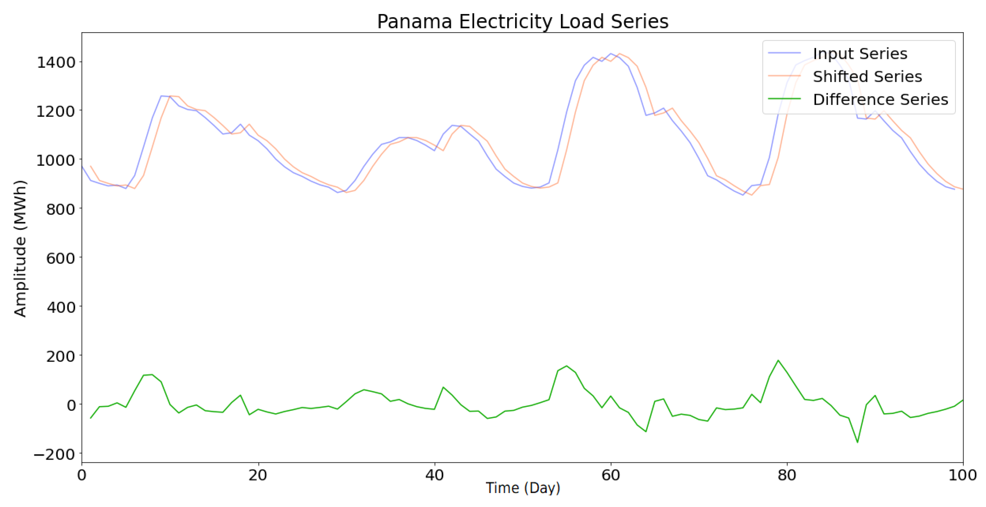In Figure 1, we report an excerpt of the electricity load from the Panama dataset. The datasets above were collected using conventional (non-neuromorphic) sensors; therefore, they are composed of real-valued data points. Because of this, to conceive an end-to-end NM system, we need to transform the data into a spike-based representation that can be processed by an SNN. We design an encoding mechanism that draws inspiration from NM vision sensors [23]. These, in a few words, produce a positive or negative event at pixel-level whenever there is a light intensity change in the scene (positive for low-to-high, negative for high-to-low). The change needs to be strong enough, i.e., above a chosen threshold, for the camera to consider it as such and thus emit an event. As a result, the NM vision sensors perform thresholding on the input, increasing sparsity in the representation, reducing noise propagation and omitting unchanging, i.e., redundant, elements. Drawing inspiration from this, our encoding mechanism transforms a real-valued input into a sequence of spikes emitted by a population of neurons. Each neuron in such a population is responsible for emitting a spike whenever the change in the signal is above a certain threshold $V_{th}^{\left(i\right)}$, both in a positive and negative direction. In other words, if the input signal has a strong enough variation from time step t to time step $t+1$, one of the neurons will emit a spike; if no change happens, or if the change is too small, no spike will be emitted, hence increasing sparsity and reducing noise, similarly to an NM camera. 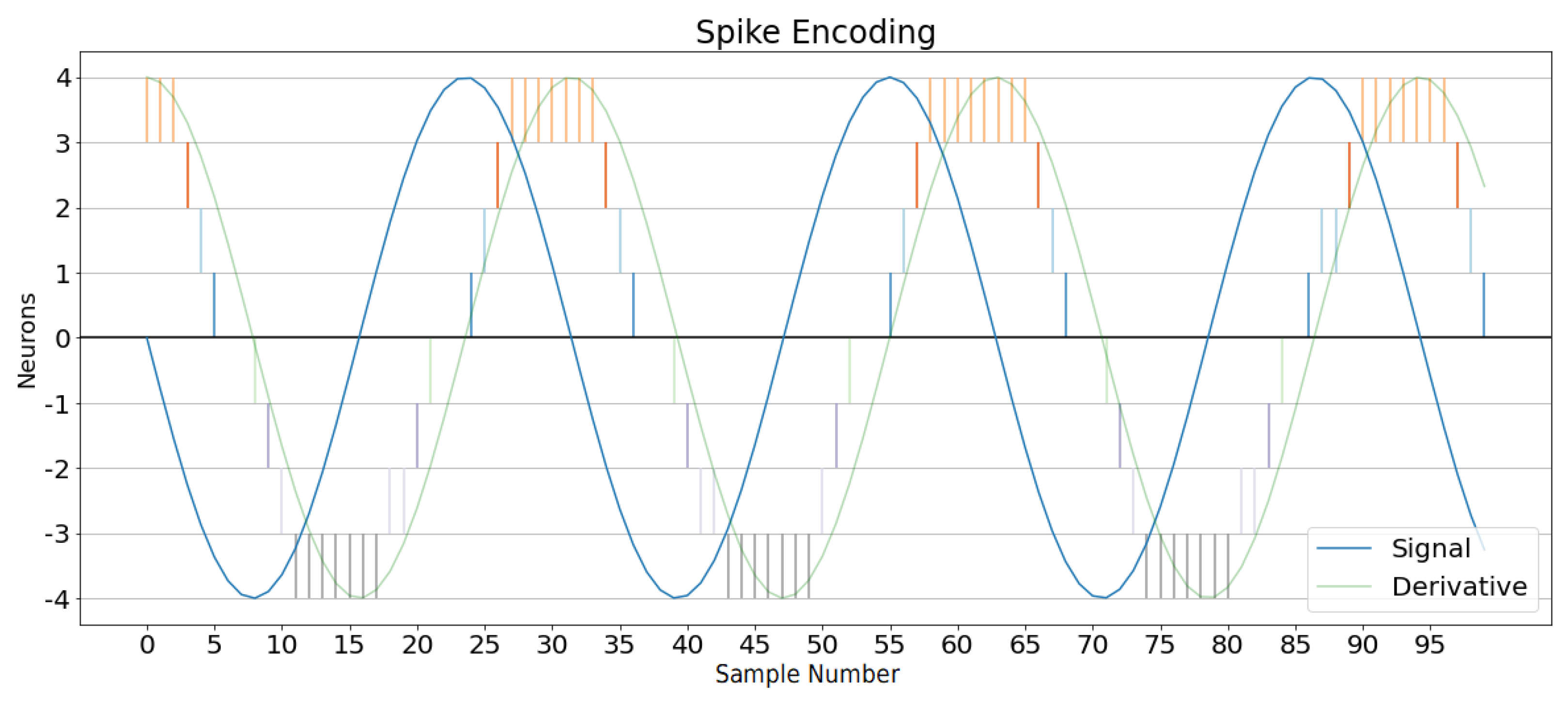In Figure 2, we provide a schematic example of our encoding system. The input is parsed by the population of encoding neurons and a spike train is produced as an output. During the encoding, neurons associated with higher thresholds implicitly inhibit those corresponding to lower thresholds. In terms of simulation using the datasets above, this is achieved by considering the difference in the input signal with a delayed version of itself by one time step. A representation of this can be seen in Figure 1 (green line).

The so-obtained encoding can be reversed by considering the threshold each neuron is associated with. Similarly to a quantization problem, the fidelity of the reconstruction of the original signal from the encoding is proportional to the granularity (number of neurons and value of thresholds) of the encoding.

In order to quantify the information loss from the encoding, in

Table 1. Mean squared error between the original signal and reconstructed signal using different encodings. Neuron multipliers should be interpreted as referring to two neurons each (positive and negative versions of each). For instance, (1, 2) with base threshold 9 refers to neurons with thresholds (−18, −9, 9, 18). The range(1, 60, step = 2) indicates a range of values starting from 1 and increasing by two up to 60. In bold, are the best MSE values from the reconstructions.

Neuron Multipliers	Base Threshold
	9	13	23	33	53
(1)	2852.88	2578.11	2033.40	1690.30	1476.04
(1, 2)	2259.65	1846.16	1187.73	910.15	944.43
(1, 2, 3)	1788.29	1328.03	731.51	576.37	814.01
(1, 2, 3, 4)	1417.18	962.62	478.96	433.10	800.42
(1, 2, 3, 4, 5)	1126.00	704.65	337.55	380.05	791.72
(1, 2, 3, 4, 5, 10)	494.50	274.81	311.93	354.15	773.62
(1, 2, 3, 4, 5, 10, 20, 30)	347.37	274.67	283.07	338.37	767.10
range (1, 60, step = 2)	509.33	938.30	2530.13	4449.87	6885.43

, we report an exploratory search of the reconstruction mean squared error (MSE) on the Panama dataset using a different number of encoding neurons with different thresholds. We used different sets of multiplicative thresholds for our encoding, i.e., each neuron was assigned a value $n\in \mathbb{Z}\setminus \left\{0\right\}$, then multiplied by the base threshold, so that the actual threshold would be $V_{th}^{\left(i\right)}=n·V_{th}$. The selection of the base thresholds was performed manually and was aided by the analysis of the value changes present in the dataset. By visualizing the count of each value change from time t to time $t+1$ (e.g., how many times the time series has had a change of 20 MWh at one time?) as reported in Figure 3, we can estimate the ranges the threshold could be varied in. In the case of the Panama dataset, there is a higher number of negative variations, but they hardly surpass the ±100 MWh. Interestingly, the minimum MSE is not obtained by using the largest number of neurons and lowest threshold, thus highlighting how threshold selection can be a crucial step. Figure 4 shows an excerpt using the parameters relative to the minimum MSE value obtained. As can be observed, the reconstructed signal follows rather faithfully the original signal, but it incurred some information loss for certain ranges of values.

2.1. Approximation of the Derivative

In its essence, our encoding method considers the average variation in amplitude of an input signal between two points in time, such that:

$$m={\displaystyle \frac{x(t+\Delta t)-x\left(t\right)}{\Delta t}}$$

(1)

where $x\left(t\right)$ is the input signal and $\Delta t$ is the chosen time step. We observe that (1) denotes the difference quotient, or the slope, of signal x around time t. Interestingly, as $\Delta t$ becomes smaller, (1) becomes an increasingly better approximation of the derivative of the signal over time as in (2):

$${\displaystyle \frac{d}{dt}}x\left(t\right)\approx {\displaystyle \frac{x(t+\Delta t)-x\left(t\right)}{\Delta t}}.$$

(2)

Thus, assuming that $x\left(t\right)$ is smooth around time t, our encoding method approximates the instantaneous rate of change, or the derivative, of $x\left(t\right)$. In practical terms, the goodness of such approximation is constrained by our choice of thresholds for the neurons, which directly affects the granularity of the encoded changes, and by the time resolution (sampling frequency) of the datasets. However, considering a single time step interval and a small enough threshold, such an approximation can be relatively accurate. In Figure 5, we intuitively show the goodness of the approximation when the input signal is a sine wave (hence with a cosine derivative). Here, the amount of change in the original sinusoidal signal is encoded by different neurons in the population. It can be seen how the activity from different neurons closely follows the cosine curve (light green).

By means of our encoding system, we obtain two major advantages. Firstly, by taking the (approximate) derivative of the signal, we are looking at its rate of change. This tells us how fast the signal will increase or decrease, regardless of its absolute value at a certain point in time. Secondly, by performing this operation, we are applying a differencing Transform to the input signal, which, in the context of time series analysis, helps increase stationarity and thus make the forecasting of the signal more precise and reliable [24,25].

2.2. Learning and Loss Functions

For the learning part of our work, we develop a simple two-layer fully connected neural network architecture using Intel’s LAVA framework [26]. More specifically, the SNN consists of two layers of fully connected Current-Based (CuBa) Leaky Integrate-and-Fire (LIF) [27] neurons, representable by the discrete system in (3):

$$\begin{array}{cc}\hfill & v\left[t\right]=(1-\alpha )v[t-1]+x\left[t\right]\hfill \\ \hfill & s\left[t\right]=v\left[t\right]\ge v_{th}\hfill \end{array}$$

(3)

where $v\left[t\right]$ is the discrete-time internal state (voltage) of the neuron, $\alpha$ is a leakage factor, $x\left[t\right]$ is the discrete-time input, $s\left[t\right]$ is the spiked value a time t, and $v_{th}$ is the threshold of the neuron. The neuron is also paired with a reset mechanism that resets the voltage to zero whenever a spike is emitted. While it has been shown that better-performing spiking neuron model alternatives might exist [11], the LIF neuron is arguably the most widely used in the literature, hence making it a good choice for future benchmarking purposes. Other than this, it can represent a valid option to increase efficiency, due to its simplicity of implementation.

We adopt an advanced version of the SLAYER learning rule to train our network in a supervised manner. SLAYER is a widely used spike-based back-propagation learning rule that allows using surrogate gradients of the neuronal spiking functions to learn weights and delays in the SNN. Furthermore, using SLAYER in the context of LAVA also allows seamless future implementations on neuromorphic chips such as Loihi 2 [28]. The standard way of utilizing SLAYER is with the loss function defined by Equations (6) and (7) in [15], named SpikeTime in the LAVA framework. Through this, the trains of target spikes and output spikes are convolved in the time dimension with a Finite Impulse Response (FIR) exponential kernel and then compared using MSE. By convolving with the FIR kernel, the loss aims to aid the resolution of the credit assignment problem through time. Further to this, we also experimented with two different loss functions that we designed specifically for this time series forecasting task. The first one draws inspiration from the concept of minimizing the differences in the inter-spike intervals (ISI) in the target and output spike train; the second one leverages the information from the encoding paradigm to decode the signal and compare the reconstructed versions of the target and output.

2.2.1. ISILoss Function

As outlined above, the ISILoss function is inspired by the concept of minimizing the differences in inter-spike intervals between two spike trains. Ideally, the ISIs should be computed for each spike train and then compared to each other. However, this is non-trivial in a back-propagation environment for several reasons. Two spike trains may have different numbers of spikes and, hence, different numbers of ISIs to compare. A possible solution for this is to adopt placeholders with pre-assigned values where the number of spikes differs. Still, it can be time-consuming and sensitive to the chosen pre-assigned value for the interval. Furthermore, this will likely include non-derivable operations, which could break the gradient calculation chain and result in unwanted behavior. For this reason, we adopted a heuristic method based on transforming the spike trains by means of derivable operations only. Specifically, we define a time-step vector R such that:

$$R=[1,2,\dots ,N]$$

where N is the number of time steps in the spike trains. We use R to re-scale each spike in the spike train by the time step at which it occurred:

$$s_R\left(t\right)=s\left(t\right)\odot R$$

(4)

where ⊙ denotes the element-wise multiplication (Hadamard product) between the spike train $s\left(t\right)$ and R. Finally, we perform a cumulative sum operation on the re-scaled spike train. To do this, we define the unitary upper triangular matrix T of size $N\times N$:

$$T=\left[\begin{array}{cccc}1& \cdots & \cdots & 1\\ & \ddots & \cdots & ⋮\\ & & \ddots & ⋮\\ & & & 1\end{array}\right]$$

and perform a matrix multiplication with $s_R\left(t\right)$. By doing this, we obtain a vector of size N that contains the cumulative sum of $s_R\left(t\right)$. The result is then normalized with respect to R.

$$\begin{array}{c}\hfill s_{cs}\left(t\right)=(s_R\left(t\right)·T)\odot {\displaystyle \frac{1}{R}}.\end{array}$$

(5)

The final loss is calculated as a mean squared error of the resulting vectors:

$$L(s_{cs}\left(t\right),s_{cs}^{*}\left(t\right))={\displaystyle \frac{1}{N}}\sum i=0N{(s_{cs}^{\left(i\right)}\left(t\right)-{s^{*}}_{cs}^{\left(i\right)}\left(t\right))}^2$$

(6)

where $s_{cs}^{*}$ denotes the target spike train, transformed as discussed. The idea behind such a heuristic is that by utilizing a cumulative sum, all the time steps present in the spike train contribute to the final loss calculation by some value (likely) different from zero. This allows us to carry some information about the cumulative time of the last spikes with each time step, and hence assign some weight to their role in the spike train, even if no spike was present.

2.2.2. DecodingLoss Function

What we call DecodingLoss is a function that builds on top of another piece of knowledge from the time series encoding: the meaning of each neuron’s firing. As a matter of fact, by means of our encoding, each neuron will be assigned a specific threshold, and will encode values that fall in the range $V_{th}^{\left(i\right)}\le x\left(t\right)<V_{th}^{(i+1)}$. We use this to reconstruct a signal starting from some output spike train $s\left(t\right)$ (see Section 2) and compare it with the decoded target spike train $s^{*}\left(t\right)$. This is possible by following a similar paradigm as in Section 2.2.1. We start by defining a vector of values that correspond to each neuron’s threshold:

$$V={\left[\begin{array}{cccccc}-V_{th}^{(M/2)},& \dots ,& -V_{th}^{\left(1\right)},& V_{th}^{\left(1\right)},& \dots ,& V_{th}^{(M/2)}\end{array}\right]}^T$$

where $V_{th}^{\left(i\right)}$ denotes the (positive) threshold of neuron i. We also define a convenience unitary vector A of size M that we can use to perform a neuron-wise addition per each time step:

$$A={\left[\begin{array}{ccc}1,& \dots ,& 1\end{array}\right]}^T.$$

In our experiments, we test both with and without this step in the DecodingLoss function. Finally, we utilized the unary upper triangular matrix T that we previously defined to perform a cumulative sum. The final reconstructed output is thus obtained as:

$$s_{rec}\left(t\right)=(A·(s\left(t\right)\odot V))·T$$

(7)

where $s_{rec}\left(t\right)$ is the reconstructed output and can be either of size N or $M\times N$ depending on whether the matrix multiplication by A was performed. Finally, the MSE is computed on the reconstructed output and target output:

$$L(s_{rec}\left(t\right),s_{rec}^{*}\left(t\right))={\displaystyle \frac{1}{N}}\sum _{i=0}^N{(s_{rec}^{\left(i\right)}\left(t\right)-{s^{*}}_{rec}^{\left(i\right)}\left(t\right))}^2$$

(8)

where $s_{rec}^{*}\left(t\right)$ denotes the reconstructed target signal. In this case, the cumulative sum has a more physical meaning than the ISILoss, as each value obtained thus directly corresponds to the value of the reconstructed signal due to all the previous changes. We can hence make a comparison of the two signals straight in the signal’s original domain and calculate the MSE loss on the final result of the obtained spikes. This theoretically opens up to the SNN learning spike trains that are not precisely the same as the target spikes, as long as the final result is still correct.

3. Results

In order to evaluate the ability of our system to learn the prediction task, we devise a series of experiments comprising a number of different settings that span across different values of parameters. In our pipeline, the data are first split into smaller segments (or windows) before being encoded. Segments can either be 128 or 256 time steps long, and each segment has an overlap of 75% with the preceding one. Using this type of windowing operation helps augment the overall dataset and helps the network build a more complete representation of the data. For each input segment, a target one is generated by looking at one time step ahead, effectively creating a challenge for the network to learn the upcoming spike. 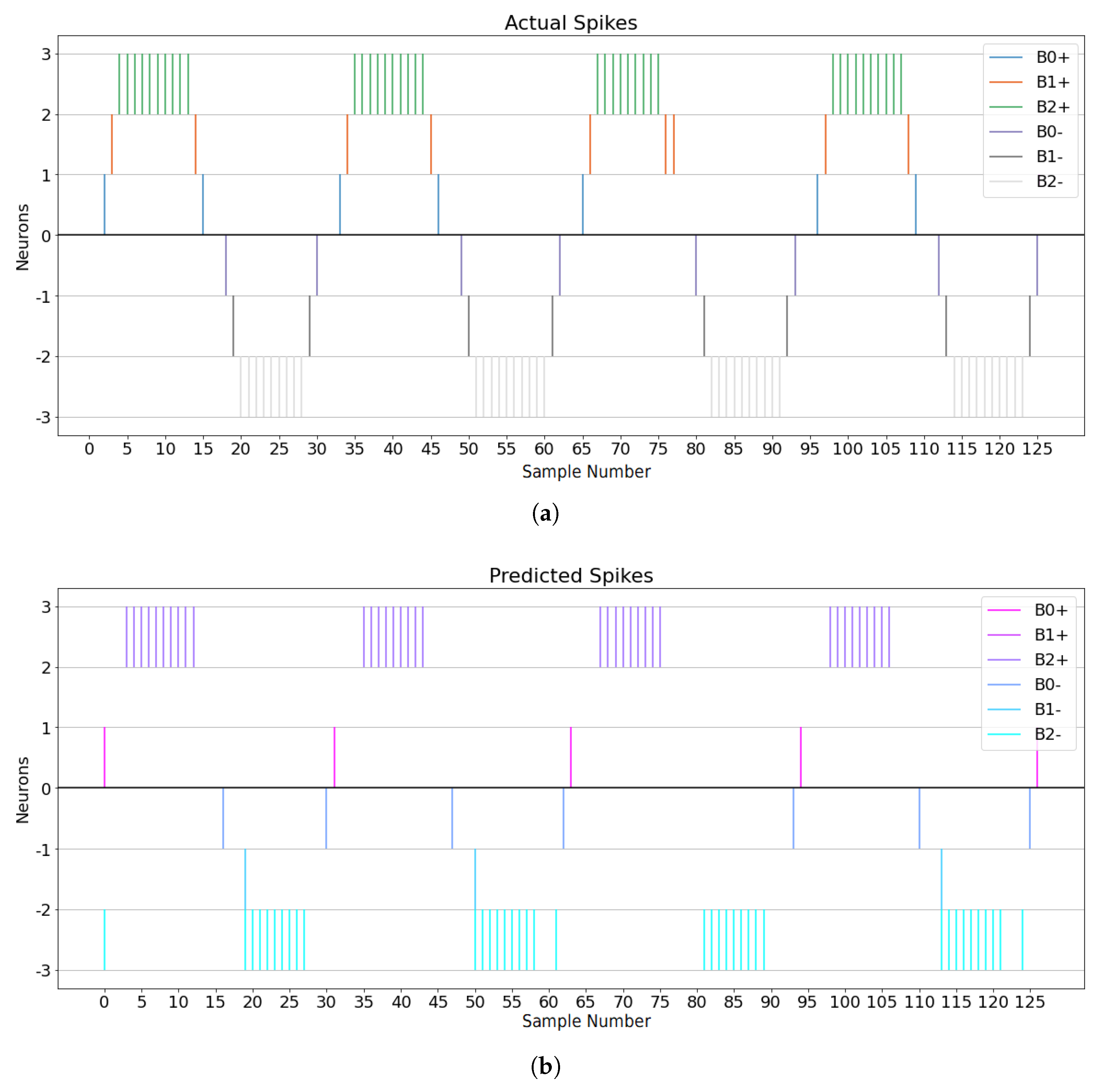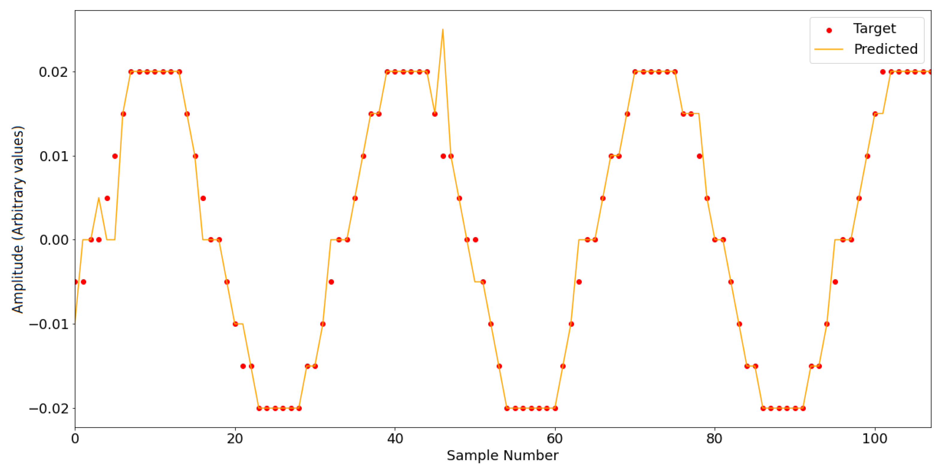A first batch of experiments was carried out utilizing a generated sinusoidal signal as an input, similar to what is shown in Figure 5, as a means to determine whether the system, as devised, would be able to learn the task. We report a qualitative result in Figure 6 and Figure 7, where we compare a target spike train with the prediction from the SNN and their respective decoded versions.

In the figures, the predicted spike train follows the periodicity found in the target train (Figure 6), aside from some mistakes, and the overall reconstruction closely matches the target one (Figure 7), thus showing how the SNN has learned to predict the next change in the signal. We therefore proceed to cross-experiment our SNN with different combinations of segment lengths, number of encoding neurons and loss functions. Each combination of parameters is repeated 150 times for a total number of experiments exceeding 15,000. To evaluate the quality of the prediction, we compare the decoded output with the decoded target sequence.

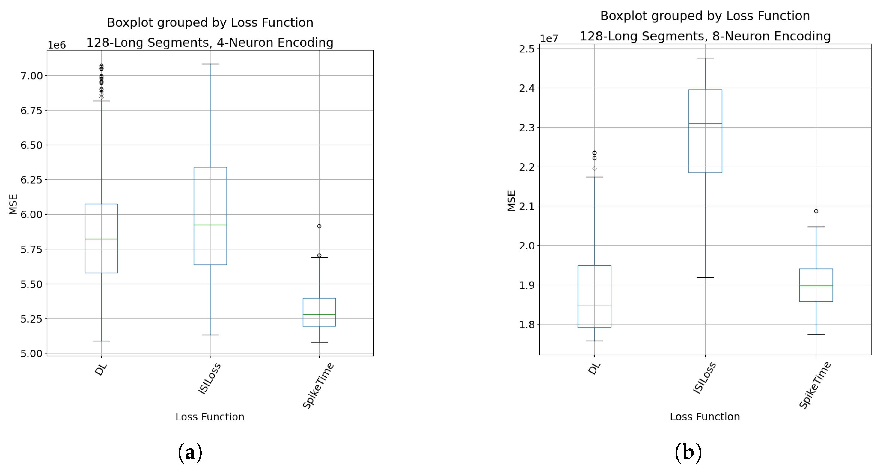
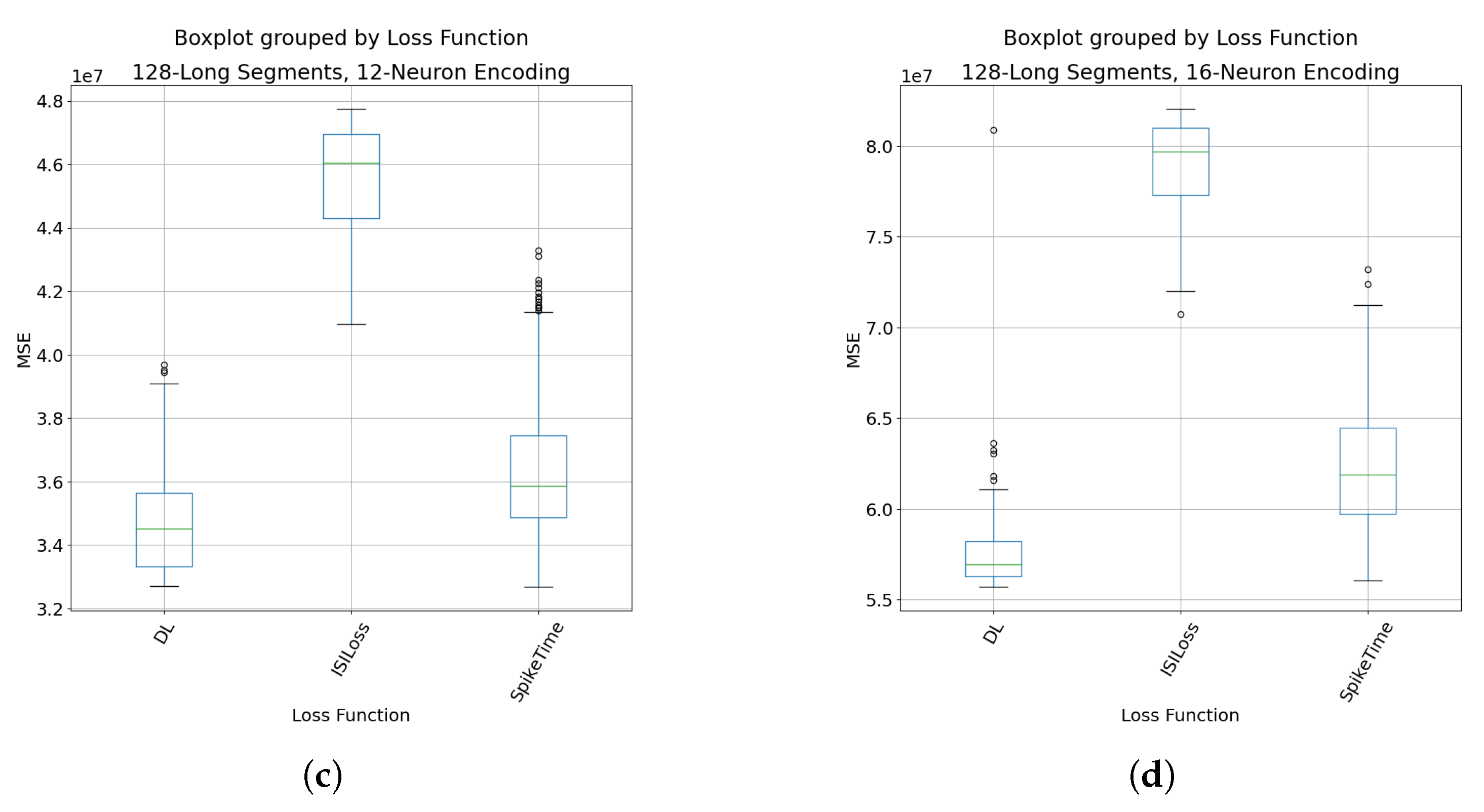
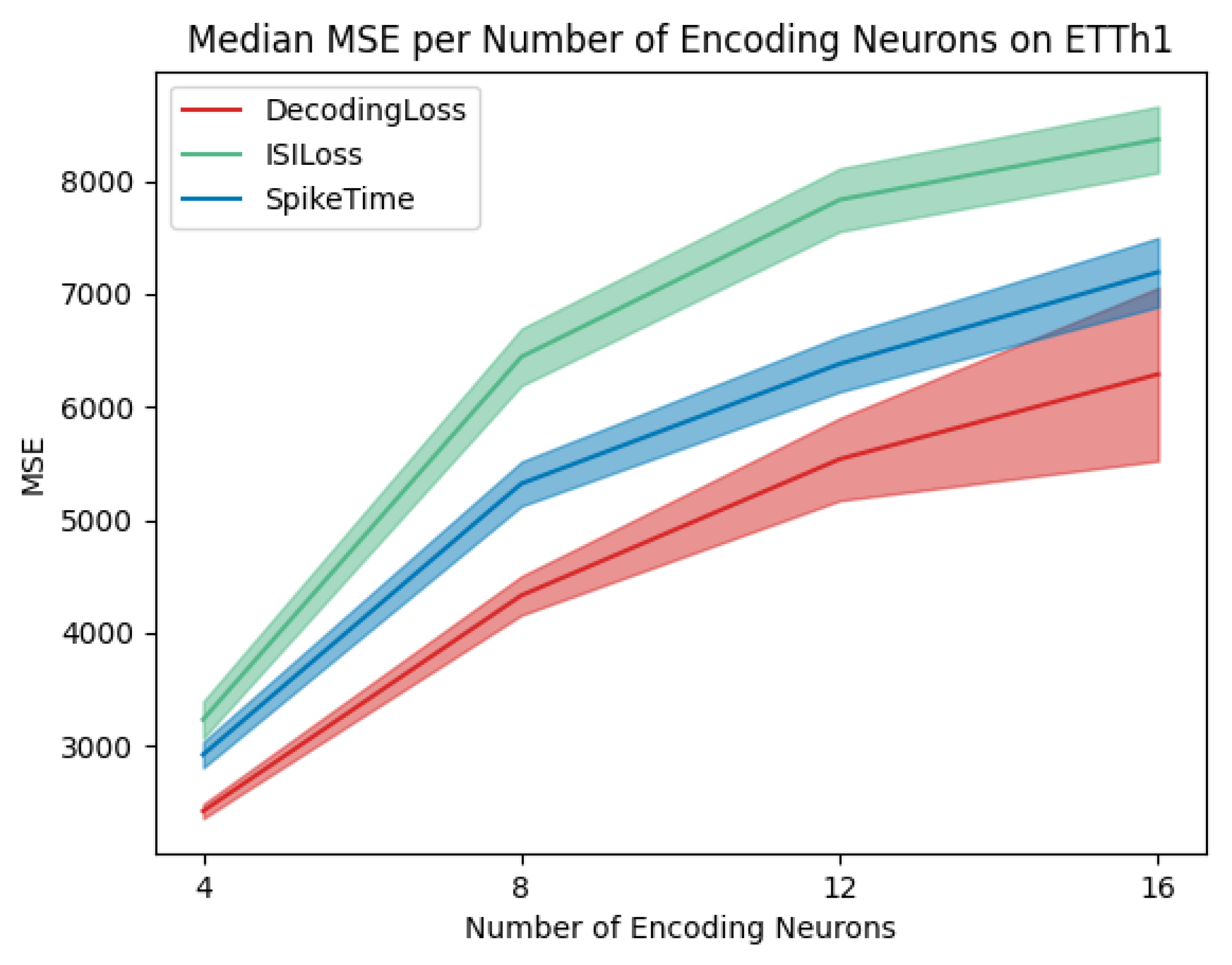
To better understand the interplay of the number of neurons with the choice of loss function on the overall performance of the SNN, we report and analyze the boxplots of the MSE of the reconstruction of the output signal with respect to the reconstructed target signal, and group them by number of encoding (and thus decoding) neurons for the case with 128-step-long segments. As Figure 8 and Figure 9 demonstrate, while the ISILoss does not seem to enable achieving better performances than the SpikeTime Loss, possibly due to an oversimplification of the initial concept to suit backpropagation needs, the DecodingLoss steadily attains lower MSE with all hyper-parameter settings, in both datasets. As the number of neurons increases, however, the overall error does too in all cases. For ease of visualization, we also report the overall performance trend across experiments with different numbers of encoding neurons in Figure 10 and Figure 11. Here, it is appreciable how the DecodingLoss achieves better results and consistently outperforms the other two counterparts. An interesting observation is in the difference in the spread of the MSE using the DecodingLoss in the two datasets. While in the Panama dataset, the results are rather consistent in terms of MSE, in the ETTh1 the spread enlarges as the number of neurons increases. Upon further analysis, we found that this could be due to the DecodingLoss assigning different and increasing values to the spikes emitted by the neurons according to the initial threshold decided for the encoding. Because of this, when the number of neurons increases, the output spikes of the added neurons are decoded into larger values; therefore, errors in the emission of spikes can become rather high for some of the neurons. This highlights the importance of the optimization of the choice of number of neurons and encoding thresholds in our setting and sets the ground for future works on researching regularization strategies for the DecodingLoss function. Finally, from the figures above, we also observe that the overall errors increase with the number of encoding neurons with all the loss functions. This is not surprising, as, given that the task is evaluated against an encoded and then decoded target rather than the original signal itself, the number of neurons that need to be trained to perform prediction is greater. In practical terms, this results in a more complex task, as would be a standard classification task with an increased number of classes.

4. Discussion

In Section 2, we described the nuances of our encoding system, and Section 3 highlighted the importance of an accurate selection of encoding parameters. What appears clear is that each dataset or use case requires an ad hoc optimization of such parameters, depending on the key elements that require capturing and the objective of the task to learn. From a broader perspective, we can identify two main limit cases. The first one concerns using two neurons only for the encoding step (one for positive and one for negative changes). Here, much of the original information could be lost due to larger changes being encoded in the same way as smaller ones. The second one is about using an infinite number of neurons with an infinitesimal threshold. By doing so, the original signal could be perfectly reconstructed. The first case would be conceivable in a scenario where the task of interest would be to merely predict whether a change is going to take place in either direction, like a simple trend prediction system. The second case (albeit requiring infinite computational resources) could be of interest in high-fidelity settings, like medical imaging, or fine-grain control systems. These two cases represent the two extremes of least computational power and least power of representation and vice versa, but in most cases, they would not arguably be acceptable and a trade-off between computational power and representational ability must be sought. By assuming another perspective, however, such a trade-off could still be beneficial to other aspects. Let us assume, for instance, that we are aware of noise and outliers being present in our data. A typical example would be an underlying current inducing small changes to be read from a sensor, or sudden surges of voltage that are not informative about the phenomenon we want to measure. In this case, limiting the largest represented value can be beneficial to our prediction system, as well as setting a minimum threshold that would nullify smaller changes. The encoding layer would therefore act as a passive filter for noise, which could otherwise potentially render the overall prediction process more difficult.

Another point worth discussing concerns the overall decrease in performance as the number of encoding/decoding neurons increases. As previously suggested, the reason behind this observation is likely to be attributed to the increase in complexity that derives from adding more neurons to the system. In the experiments that we devised, an input sequence is encoded into a spike representation and is fed to the SNN. The SNN processes said sequence one time step at a time and outputs one or more spikes that are apt to predict what the next time step’s value is going to be. The predicted value (spike) is thus compared with the target value depending on the choice of the loss function, and the quality of the prediction is evaluated by comparing the decoded versions of the two. The output of the network, therefore, is not directly compared with the same original time series values in every case, but with its encoded and then decoded version from time to time. This effectively equates to posing a more difficult task to the SNN every time the neuron number increases. As discussed above, fewer encoding neurons would naturally incur a higher quantization error due to their limited representational power, therefore by utilizing the same neurons and comparing them against the original time series’ signal, the MSE should be expected to be higher. Instead, by comparing them with an encoded-decoded version of it, we disregard the quantization effect and therefore simplify the task. At the same time, we should expect more neurons to incur lower errors, as they could potentially create representations that resemble the original signal more closely. However, for the same reason as earlier, the overall error sits higher than the cases with fewer neurons. Analyzing more in-depth the causes of such effects will be the focus of future research on this topic. Finally, we focus on the potential effects of utilizing the DecodingLoss as opposed to the SpikeTime loss on the output of the SNN. The SpikeTime loss is built to promote learning to match exactly the position (in terms of which neurons have to emit it) and the timing of the spikes. Because each spike is reached by building up a neuron’s internal membrane potential, errors are assigned through time, and not just at the moment of the emission of the spike (i.e., also the preceding time steps are affected to a certain degree). When it comes to the DecodingLoss, instead, the focus is on learning a sequence of spikes that, once decoded, achieves the same result as some reference value, or signal, over a period of time. This subtle difference makes it such that the SNN does not necessarily need to learn exactly the timing and position of some spikes, so long that the resulting decoded signal is good enough. This leaves more flexibility to the SNN, which has therefore access to a greater number of minima to reach, as the combinations of spikes that can achieve this are larger. The degree of freedom allowed by the DecodingLoss is, however, modifiable depending on the modeling needs by including a decoding window in the formed of a modified triangular matrix. If a closer resemblance to the target spike train as-is is required, the decoding window can be reduced accordingly to achieve this result.

Limitations

The presented work envisions an end-to-end sensing and prediction system for time series, but it does come with certain limitations. Neuromorphic technologies have seen a surge in interest and proactive research, but remain in the prototyping phase, lacking a general consensus on best practices. The number and types of sensors and neuromorphic chips are limited, hence the necessity for an encoding layer, as not all data types can be directly sensed by an ad hoc neuromorphic sensor. This requirement for data conversion into spikes or events introduces an overhead that would not exist if sensors with the same sensing capabilities were available. While this might be acceptable in the current stage of research, it adds an extra layer of complexity.

Moreover, the power and time efficiency advantages highlighted in the literature rely on the vision of an implementation of algorithms within a fully end-to-end neuromorphic system. However, designing or finding such a system remains challenging. As a result, algorithms are often evaluated through simulations, and their power and time efficiencies are often, although not always, estimated based on specific criteria rather than measured directly.

Additionally, this work focuses on predicting one time step ahead in the time series to demonstrate a proof of concept. More conventional applications typically require predictions of multiple time steps ahead, which will be addressed in future research on this topic.

5. Conclusions

In this work, we approached the problem of time series forecasting using SNNs. We introduced a novel encoding scheme inspired by the NM vision sensors and showed its affinity with the concept of the derivative of a signal by means of a purposely built sinusoid series. The neuron encoding, in fact, closely resembles a cosine signal. To demonstrate an SNNs ability to learn to predict the next upcoming spike in a so-encoded series, we build a relatively simple SNN and train it using the SLAYER learning rule. Further to this, we develop two loss functions to be paired with SLAYER and our encoding system, the ISILoss and the DecodingLoss. We perform an exploratory analysis of our encoding system, and test our solution on a number of different parameter configurations, so as to obtain more insights on the interplay amongst them. From our results, we deduce that our encoding scheme can effectively be employed for time series data to be learned by the SNN and that different levels of granularity in the encoding resolution can yield different results. In particular, we discuss the relationship between the number of neurons in the encoding population and the thresholds assigned to them. We also observe that the ISILoss does not perform at the same level as the other two tested loss functions, potentially due to the approximation of the original concept into a version that is much simpler and more amenable to backpropagation. At the same time, our results show a higher consistency in obtaining better prediction results when employing the DecodingLoss rather than the SpikeTime when used in combination with our encoding system. Due to the nature of the DecodingLoss, this suggests that it might be beneficial not to force the SNN into learning a predefined set of spikes to represent some value, but that it could instead prove better to let it find appropriate ways to do so from the point of view of the reconstruction accuracy. To conclude, we have proposed a proof-of-concept novel NM approach to the forecasting of time series. The encoding leverages ideas from NM cameras, concepts from derivatives of signals, and advantages from the differentiation process, which helps in rendering the data more stationary. Our results demonstrate an ability to learn future spikes from the input data, however, this represents just a first step towards further developments in this direction. Future research will focus on optimizing the loss functions and the encoding system to better learn and represent the data according to the task at hand, and on integrating readings from a number of sources to implement multi-variate time series forecasting.