1. Introduction
The rapid advancement of technology, and the increasing dependence on computational systems, has generated concern over the security of these systems from adversarial agents. In recent years, technology has brought about a profound metamorphosis in our daily lives as a society. The influence of disruptive technologies such as Internet of Things (IoT), 5G networks, artificial intelligence (AI), machine learning (ML), and quantum computing is leaving an unprecedented mark on the world [
1,
2]. On one side, we can celebrate having more digital tools, more information all the time, and more facilities in a digital society. On the other hand, the advent of these potentially transformative technologies carries significant ramifications for cybersecurity [
3,
4].
The prevalence of diverse cybersecurity threats in recent years cannot be understated when evaluating the safety of a system. While modern techniques for preventing the spread of malware have proven to show some effect in specific domains, it is well established that their failures continue to result in damages exceeding billions of dollars. In 2020, losses due to Internet crime exceeded USD 4 billion, up from USD 3.5 billion in 2019 [
3,
5]. This statistics, however, only represents reported losses with directly traceable and quantifiable measures—it does not represent the true scope of potential damage.
Of these sharp dangers, malware ranks among the most significant. Financial incentive among malware developers is so extreme that some 350,000 new malware samples can be discovered in a single analysis [
6]. Each and every sample represents a unique challenge for detection and classification that far outpaces the expertise of the already limited professionals in the field.
Unfortunately, the scope of traditional approaches for malware detection is incapable of keeping up with the exponential development of recent malware [
4]. Promisingly, AI methods may have the answer [
3,
7,
8]. ML has demonstrably worked on capturing the essence of malware samples to effectively combat the growing threat [
9]. These methods are dynamic in their capacity to identify previously unknown dangers [
4], offering a promising general-case solution to protect against malware.
In this paper, we present an analysis of three widely used ML algorithms: artificial neural networks (ANNs) [
10], support vector machines (SVMs), and gradient boosting machines (GBMs), for malware detection with computational resource constraints. Our research is based on the evaluation of these algorithms’ key result metrics using a publicly available dataset of malware samples [
11].
We used program metadata, obtained from our VirusShare dataset, to train and test the algorithms. The metadata provides valuable information on the behavior and characteristics of malware, which enables the algorithms to detect new or previously unknown malware. We also incorporated strategies for reducing each model’s memory footprint in the hopes that they may be adopted by the low-resource hardware frequently found in IoT [
1].
The structure of this paper is as follows:
Section 2 details the state of the art, previous research, and the modern technologies adjacent to our work.
Section 3 covers the materials and methods implemented to develop the experiments and how the results are obtained.
Section 4 presents the produced results. Then,
Section 5 and onward offer a comprehensive analysis of the meaning and significance of our results, where our research is situated, and our conclusions.
2. State of the Art
Researchers have extensively explored ML techniques to enhance malware detection, especially within specific domains.
Table 1 presents a selection of papers that are related to malware detection using ML.
The portable executable (PE) file format, which is standard for Windows executable files, has attracted attention for malware analysis. ML demonstrates robust efficacy in identifying malicious PE files [
12,
13], with some studies leveraging deep networks [
14]. Emphasis is placed on feature extraction from PE files for enhanced detection [
15]. The rapid expansion of Android devices also instigated research into malware detection on this platform using both machine and deep learning, which yields high accuracy rates [
5,
16,
17]. The integration of static and dynamic analysis methods, like OPEM, offers increased detection capabilities [
18]. Feature extraction, specifically focusing on opcode frequency, emerges as pivotal in distinguishing malicious from benign software [
19]. Comparative studies benchmark the success of ML-based methods against traditional antivirus systems [
20], while others explore dataset bias and innovative techniques like image processing applied towards the goal of malware pre-processing [
21].
Table 1.
State of the art in machine learning for malware detection.
Table 1.
State of the art in machine learning for malware detection.
| Topic | Authors |
|---|
| Portable executable (PE) file-based detection | Mithal et al. [12], Malik et al. [13],
Vinayakumar et al. [14], Baldangombo et al. [15] |
| Android malware detection | Amin et al. [5], Milosevic et al. [16],
Agrawal et al. [17], Feng et al. [22],
Pan et al. [23] |
| Combining static and dynamic analysis | Santos et al. [18],
Mangialardo et al. [24], Jain et al. [25] |
| Feature extraction and reduction | Rathore et al. [19] |
| Comparative analysis and literature review | Fleshman et al. [20],
Vinayakumar et al. [21] |
| General overview and robustness in dynamic analysis | Ijaz et al. [9], Or et al. [26] |
| Behavioral data and short-term predictions | Rhode et al. [27] |
| IoT device malware detection | Baek et al. [28] |
| Vulnerabilities and evasive techniques in IoT | Fang et al. [29] |
Multiple approaches have been deployed to enhance the prompt identification of diverse malware types, as detailed in [
30]. The taxonomy of malware analysis distinguishes between static and dynamic analyses. Static analysis centers on identifying malicious files without execution, while dynamic analysis involves the initial execution of the file. A hybrid strategy integrates the elements of both static and dynamic analyses. Research in malware detection showcases a dual emphasis on feature-specific analysis and the integration of various tools.
On one hand, static analysis allows researchers to focus on unique malware characteristics, such as those found in ransomware, demonstrating the adaptability of this analysis [
3]. The literature frequently discusses refining this strategy by enhancing strengths and simplifying metrics [
31,
32]. On the integration front, the development of comprehensive tools enhances malware analysis. Examples include platforms offering comparative insights into different detection tools in the context of static analysis [
33]. Specifically, for Android-based malware detection, AndroPyTool stands out as a multi-tool integrative system, exemplifying the strength of unified analytical frameworks [
34].
On the other hand, dynamic analysis is an integral facet of malware detection. The robustness and intricate aspects of this method have been underscored by various researchers, with some highlighting the benefits of incorporating ML for an enriched analysis [
9,
26]. Taking a more specialized approach, certain studies advocate for the utilization of short-term behavioral data snapshots to differentiate between malicious and benign software. Techniques like these offer swift and accurate detection, successfully navigating hurdles such as code obfuscation and latency in data capture [
27].
The application of malware detection extends to IoT devices given their ubiquity and connectivity [
2]. As evidenced by the literature, they are tempting targets for malware programs [
1,
28]. With the spotlight in this domain, there is research on two-stage hybrid malware detection schemes which merge static opcode analysis with dynamic methodologies tailored for IoT environments.
As malware detection evolves, evasion techniques also evolve [
29]. In some cases, researchers delve into the vulnerabilities intrinsic to deep learning-based static malware models, utilizing Windows PE features. By exploring adversarial sample generation via deep reinforcement learning, they illuminate the ongoing tug-of-war between malware authors and detectors.
This consolidated view captures the breadth and depth of contemporary research in malware detection, demonstrating the multifaceted approaches and innovations driving this domain. It is evident from the literature that the domain of malware analysis via ML, aided by adjacent detection mechanics, is both large and successful in producing experimental results. To foster new development in this field, the aim of our paper is tailored towards exploring the efficacy, limitations, and capabilities of low-parameter ML models. The dependence on cheap hardware for modern service infrastructure necessitates advancements in lightweight malware detection, and as such, our experiments are presented with this in mind.
3. Materials and Methods
In the following subsections, relevant information regarding the process of conducting the experiment will be presented. A desktop application, hosted in our public repository, has been developed in order to facilitate the replication of the experiment [
35]. The GitHub repository contains all the files, datasets, and resources required to build and run the application. This includes the codebase, configuration files and dependencies needed for successful execution.
3.1. Dataset
The dataset used in the experiment was generated using parameters from PE format files, whose content was analyzed and subsequently classified as malicious software on the basis of the VirusShare public data and evaluation techniques. The files were collected from the malware collection at
virusshare.com accessed on 8 November 2022 [
11], from which only PE files with extractable characteristics were retained. Subsequently, they were analyzed using the Pefile tool. Pefile is a cross-platform tool written in Python for analyzing and working with PE files. In PE files, most of the information contained in the headers is accessible, as well as details and data for executable sections. Relevant information for malware identification, such as section entropy for packer detection, was extracted from these files.
In total, the dataset contains 57 attributes. The attribute ‘legitimate’, obtained from VirusShare’s data, is used for the ground truth of the experiment (see
Table 2). The dataset consists of 152,227 samples of program metadata, among which 138,047 are considered for our experiments; while 14,180 samples were discarded due to empty, corrupted, or incomplete data. Among the 14,180 samples, 13,289 corresponded to corrupted data and 891 samples were too obfuscated to use. The decision for removing excessively obfuscated samples was motivated by an interest in avoiding the sparsity introduced. The missing entries are deemed unnecessary for the purposes of this experiment. Of the 138,047 remaining program metadata samples, 96,724 represent malware metadata and 41,323 represent legitimate program metadata. The distribution is approximately 2.3:1 as a ratio of the malware program to legitimate program metadata.
A complete and comprehensive analysis of the dataset is available in our project repository [
35]. It contains information regarding the meaning of the metadata, as well as a broader statistical analysis of the elements contained within.
3.1.1. Data Preprocessing
To proceed with the experiment, we decided to remove 14,180 malware samples from our dataset. Out of these, 13,289 were excluded because they were damaged in some way, while 891 were left out due to being too obfuscated for analysis. Adding these incomplete samples had negative effects, reducing both the accuracy and the memory efficiency of our models. Initially, we tried to compensate for the missing data by filling in gaps with zeros, thus introducing sparsity into the data. We found that our models needed more complex adjustments to accurately deal with the subsequent bias. Our early calculations indicated that the sparsity introduced by the zeros of these incomplete samples would have increased our memory usage by a surprising 31% to address less than 9% of the dataset. In the case of the SVM, the model with the least internal parameters, the accuracy fell by around 11% with a staggering 158% increase in false positives (incorrectly identifying safe programs as malware). Moreover, we found no proof to suggest that our other models would have benefited from including these samples. In fact, doing so might have misled the models into incorrectly associating random data patterns or zeros with malware, which is not always the case. This concern was confirmed by further analysis, which showed that the rate of false positives increased by up to 22% even in our most robust model, the ANN.
3.1.2. Statistical Measures of Data
In
Table 3 and
Table 4, we present the general statistical tendencies measured for each of the attributes of the dataset. This report does not include all the metadata as it merely serves to represent the methodology. The factors considered are the element counts (which are equal among all fields), statistical mean, standard deviation, minimum, and percentiles per attribute.
3.1.3. Value Correlations
To understand the behavior of each attribute relative to the ground truth, we compute the correlations. The role of each value becomes clearer once evaluated through this, as seen in
Table 5. Certain attributes from the dataset might have a high correlation but they cannot be feasibly scanned in real-world samples. The unfortunate situation is the result of overfitting from the dataset, because it incorrectly assumes that it is representative of broader real-world software.
It is essential to understand the meaning of each dataset value to reproduce results with newly generated data. Below, there is an explanation of the most important attributes in the dataset, selected from the elements with high absolute value correlation to the ground truth.
Machine (positive correlation): This property indicates the architecture of the target machine for which the binary was compiled (e.g., x86, x64, ARM). A hypothesis could be that certain architectures are more commonly associated with legitimate software than with malware, or vice versa. This, however, might prove problematic as it may not be necessarily indicative of real-world malware samples.
SizeOfOptionalHeader (Positive Correlation): The size of the optional header can vary based on the format or version of the binary. The property attempts to classify this information. One possible insight comes from the fact that legitimate software may contain more standardized, recent formats.
MajorSubsystemVersion (Positive Correlation): Indicates the major version number of the required subsystem. Legitimate software might be updated more frequently to use the latest subsystems. So, malware might target older versions which are more vulnerable subsystems.
SectionsMaxEntropy (Negative Correlation): Entropy is a measure of randomness or unpredictability. This measure is indicative of either obfuscation or encryption. These techniques have valid use-cases for legitimate programs, but they are frequently used by malware to protect the nature of a payload.
DLLCharacteristics (Negative Correlation): This represents certain flags or attributes set in the binary related to DLLs. Malware might use certain methods of obfuscation and dependency to achieve persistence or evasion.
SizeOfStackReserve (Negative Correlation): This property defines the amount of memory required in the stack for the program to execute correctly. It is possible that malware programs might manipulate this information for any number of reasons. The more likely candidates include detection evasion or simply exploit vulnerabilities related to the stack of a system.
ResourcesMaxEntropy (Negative Correlation): Similarly to SectionsMaxEntropy, high entropy in resources might indicate that malware is either embedding encrypted data or obfuscated data.
3.2. Representation
We also performed an analysis of each attribute to determine the distribution of the data. The objective is to determine which normalization strategy might most accurately depict the information. In this step, we discard string-based fields and entirely focus on a numerical approach. To pre-emptively select the normalization strategy, we employ an algorithm that factors in statistical tendencies to form a conclusion.
As evidenced in
Table 6, we most frequently observe the selection of a robust scaling strategy by the algorithm. This strategy is crucial for handling outliers, which is logical for this dataset because values frequently fall outside a simple norm.
After the algorithm evaluates the basic tendencies of the data, we manually analyze column histograms to determine the most suitable normalization strategy. One common observation is that bimodal or trimodal clusters manifest frequently in the data. By human inspection, we determine where to consider remapping bimodal distributions into simpler integer values such as binary or ternary. Once factored in, we produce an attribute-by-attribute normalization of the data on the basis of machine and human inspection. We believe this effectively normalizes the data for the subsequent models to train on.
3.3. Selection of Algorithms
The following algorithms were used to classify the processed dataset: artificial neural networks (ANN) [
7,
36] with the internal structure determined by a genetic algorithm, support vector machines (SVMs) and gradient boosting machines (GBMs). The hyperparameter settings for both GBM and SVM were determined by testing and iterative experimentation to generate optimal results with respect to memory optimization. To compensate for different ratios of malware to legitimate programs, and to ensure a reduction in false negatives, the penalty weights were modified based on the type of program evaluated. L1 regression was used to reduce the trade-off of extreme outliers for both legitimate and malicious programs.
3.3.1. Neural Network Optimized through Genetic Algorithm
Genetic algorithms have been used in combination with ANN for many years [
37,
38,
39] to optimize the architecture of the ANN. It has been shown to be effective in finding high-performance solutions to complex problems. However, despite the potential of this technique, there is a lack of research on methods for constraining the complexity of the neural network architectures generated by a genetic algorithm [
40]. Given the importance of automatically selecting ANN, it is also necessary to develop techniques for preventing overfitting. Here, we propose a novel approach based on genetic algorithms to select an optimal ANN structure. This approach incorporates a constraint on the depth of each network architecture as well as the parameters. This approach offers a number of benefits over existing methods, and can help to improve the performance and robustness of the generated ANN.
Let
X be an ANN composed of
N layers such that
. Where
represents the input layer, and
represents the output. This architecture corresponds to a multilayer neural network and backpropagation, see
Figure 1 [
7,
36].
When an ANN is deployed, there must be a direct relationship between and the input parameters P such that for any positive real value of Q. Next, we define as the final layer output of the ANN. Depending on the type of answer we want, we modify its size. Roughly speaking, each possible answer that the network can give represents another neuron in this layer. If we are trying to classify an input into one of three classes, then .
Let
A be the architecture of the network such that:
We can see that A simply represents the inner layers of the ANN X. Designing the inner layers is significantly more challenging than the input and output layers. We need to consider several aspects such as: (i) the length of A; (ii) every value ; and (iii) to evaluate how each one plays a meaningful role in the convergence of the output.
To determine an optimal value of A, a genetic algorithm is used. We define a genetic algorithm G, a population P, a chromosome C, a fitness function F, and a mutation rate M as a tuple .
Let such that all are subject to the previously defined ANN definition.
Let
where the resulting operation yields:
and
A follows the previous definition.
Let M be a fixed mutation rate such that .
Let
where
C is the previously defined chromosome. We define the fitness function as:
For G, we attempt to find a from P that minimizes F. If there is no that sufficiently satisfies F, we update P by replacing the lowest performing p with children bred from the highest performing p. We define the breeding procedure as a random selection of two parent solutions. We randomly select two chromosomal characteristics, and swap them, subject to M, to create a child which replaces the next worst performing p. We repeat the breeding procedure until we have replaced a sufficient proportion of the population. We repeat the iterations until we have sufficiently minimized F.
3.3.2. Gradient Boosting Machines Optimized for Limited Resources
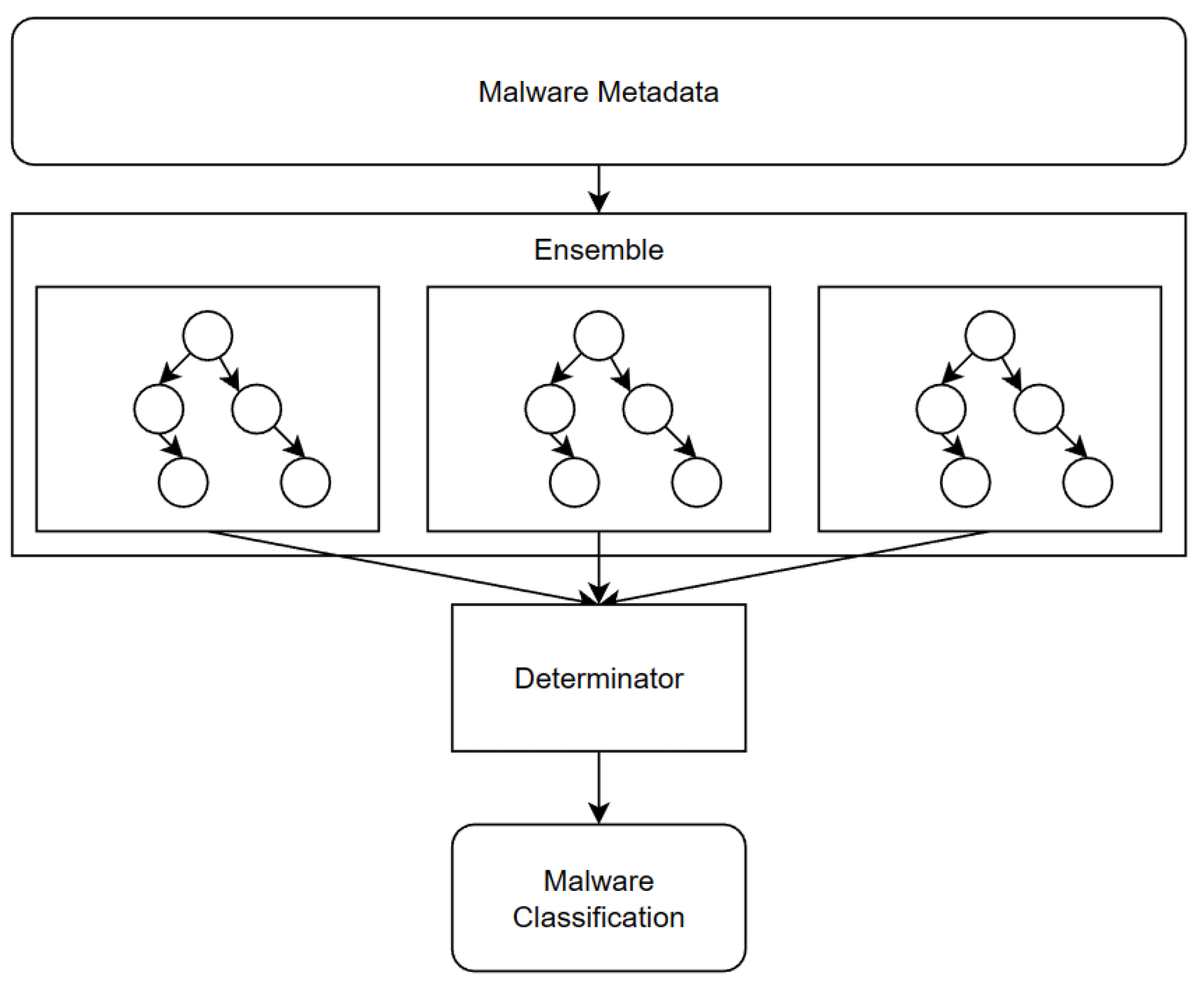
In this study, the efficacy of a GBM was also investigated as per the architecture detailed in
Figure 2. To optimize the GBM’s performance for the dataset, a grid search was implemented. This search was designed to explore a comprehensive range of hyperparameters, specifically focusing on five key elements: the number of estimators, learning rate, maximum tree depth, minimum samples required to split a node, and the number of iterations without improvement before early stopping.
Table 7 delineates the values evaluated for each hyperparameter.
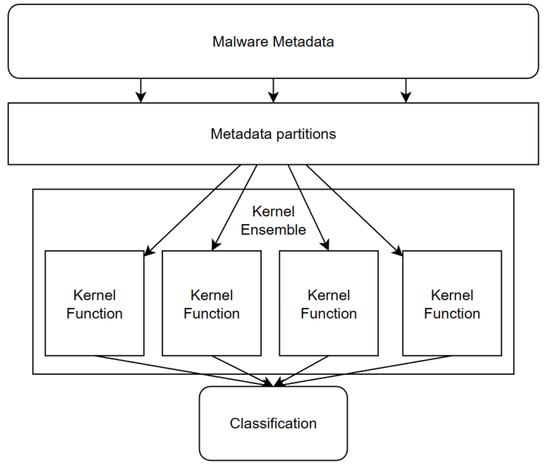
3.3.3. RBF Support Vector Machine
With a similar intent as the GBM, a SVM was implemented to explore results in low-parameter models. The interest of SVM lies in its capacity to approximate the ground truth with the assumption that it is close to linearly separable. To obtain the best hyperparameters here, C and gamma were explored exhaustively as seen by the values in
Table 8. The architecture is briefly detailed in
Figure 3.
3.4. Training and Evaluation
In our experiment, we focused on the evaluation of machine learning algorithms, centering our assessment on two metrics: the accuracy and loss of the model in its evaluation phase and its size. The objective of our study was twofold. Firstly, we aimed to ensure that the models generated are of the highest accuracy, ensuring that predictions and classifications are as close to the actual outcomes as possible. Simultaneously, we were keen on ensuring that these models are lightweight, maximizing their efficiency without compromising on their accuracy.
To facilitate this, we employed a data splitting strategy, segmenting the dataset into training and testing subsets. Specifically, 80% of the entire dataset was allocated for training, while the remaining 20% was set aside for testing. Furthermore, within the training subset, we earmarked 15% for validation. This validation set plays a crucial role, especially in tuning the model parameters and preventing overfitting, which can adversely affect the model’s performance on unseen data.
For the ANN component of our experiment, we leveraged the binary cross-entropy as our loss function, a common choice for classification tasks. The model was compiled using the Adam optimization strategy, which is favored for its efficiency and quick convergence in training deep learning models. The combination of these choices aimed to achieve optimal results in the training and evaluation phases of our study.
3.5. Experimental Setup and Hardware Configuration
To carry on the experiments, Google Colab was employed to accelerate the training process. The programming language Python 3.9 was selected in conjunction with libraries commonly utilized in data analysis and machine learning tasks. These libraries encompassed scikit-learn for the preprocessing of data, selection of features, and evaluation of models; matplotlib for the purpose of data visualization; numpy for performing numerical computations; tkinter for the creation of a graphical user interface; pandas for the manipulation and analysis of data; and TensorFlow for the construction and training of neural network models. The integration of these libraries yielded a resilient software ecosystem, thereby facilitating the efficient analysis, modeling, visualization, and user interaction throughout the entirety of the experiment.
4. Results
In this section, we present the results of the tests performed on each of the proposed ML models (ANN, SVM, and GBM). Our objective is to compare and evaluate the performance of the models in terms of accuracy and loss as well as resource requirements for the classification to take place.
Table 9 demonstrates the best raw results for each of the three ML models implemented, in bold are the best results. The results clearly demonstrate that each of the three models can be effectively implemented in some capacity towards the goal of classification. We also introducing a false positive ratio (
) and false negative ratio (
), defined, respectively, as:
where
denotes false positives,
denotes true negatives,
denotes false negatives, and
denotes true positives. These metrics are essential as they allow us to further compare the rates and the nature of the models’ failures.
denotes the likelihood that a model will produce a false positive classification. Meanwhile,
denotes the likelihood that a model will produce a false negative classification. The values range from 0 to 1, where 0 indicates a perfect model and 1 indicates an inverse relationship to ground truth. Though it would be ideal for models to have values close to 0, our target is to ensure that models have an
below 0.05 and an
below 0.1. Loosely speaking, this would suggest that the models are twice as likely to accidentally flag false positives as they are to flag false negatives. In the case of malware analysis, this is consistent with a preference towards caution when handling foreign software.
4.1. ANN Results
Figure 4 demonstrates the drop-off in performance of the ANN as the genetic algorithm constraints increase to favor reduced parameters, and subsequently, memory constraints. While it is clear that, as alpha increases, so does accuracy, and the diminishing returns for values beyond 0.6, with an accuracy of 93.44%, may indicate that there is no reason to exceed it. Values of 0.8, with an accuracy of 94.74% or higher seem to align with overfitting, see confusion matrix in
Table 10; while values below 0.5 offer far too little precision in the context of malware analysis. A key demonstration of the efficacy of this model lies in the inspection of the
and
at an alpha of 0.6. Of the three models tested, the ANN has the lowest ratio of False Negatives and False Positives, demonstrating a clear competence in evaluating samples. This aligns with the hypothesis that the genetic algorithm provides a useful framework for improving the ANN.
4.2. SVM Results
The strength of the SVM model is that it requires less tuning to determine whether or not it is useful. The results of this experiment, with an accuracy of 91.07%, indicate that the model, while using the RBF kernel, yields useful results in this domain, see confusion matrix in
Table 11. The reduced parameters of this model offer an advantageous performance in inference and training when compared to more sophisticated models such as the GBM ensemble and the ANN. An important consideration of the SVM is that its
and
values stand out among the three model options. With an
of 0.158 and an
of 0.053, it is higher than both the GBM and ANN. This indicates that the model is less flexible than its counterparts when handling legitimate programs—a consequence of it being a lighter model.
4.3. GBM Results
For the case of the GBM models,
Figure 5 shows the behavior of the accuracy as preference towards accuracy increases. The best accuracy is 0.92 (92%), see confusion matrix in
Table 12. The value of the preference towards accuracy is computed as
. This, however, comes with a negative memory overhead. The critical points of the models occur at 0.64 and 0.79, where the largest differences in model accuracy occur. And, 0.79 appears more favorable for this experiment as it is not significantly larger than the former point while consistently providing significant improvements. For the case of malware analysis, we consider that an accuracy of 0.85 or lower does not offer sufficient coverage, especially when considering the risks of the dataset not representing the entire space of both malware and legitimate programs. With an
of 0.050, the GBM is close behind the ANN in managing the detection of malware. Interestingly, the
of 0.133 indicates that the model has a significantly higher likelihood of falsely flagging a legitimate program than the ANN when accounting for accuracy. With a sharp skew towards false positives, this suggests the model would be better suited as a first line of analysis via filtering as opposed to the conclusive classifier.
5. Discussion
The comparative analysis of the ANN, SVM, and GBM models in the context of classifying program metadata as malware or legitimate provides valuable insights into the strengths and trade-offs of each approach. This discussion synthesizes these findings and offers practical considerations for their application.
The ANN model demonstrates the highest level of accuracy found, particularly when the alpha parameter is finely tuned. However, there is a noticeable trade-off between accuracy and computational efficiency. The diminishing returns observed beyond an alpha value of 0.6 suggest that this might be the optimal setting for balancing accuracy with resource utilization. This balance is crucial in the context of malware analysis, where both precision and efficiency are paramount. However, the lengthy training time (over 13 h on Google Colab) highlights a significant area for optimization in future research, perhaps through more efficient training algorithms or parallel processing techniques. The ANN model is best suited for environments where high accuracy is needed and computational resources, especially time, are not a primary constraint. The alpha value of 0.6 should be considered as a starting point for achieving a balance between efficiency and accuracy. On top of offering leading accuracy over the competing models, its and scores are excellent indicators of the fact that the model was most correctly generalized from the dataset. This suggests that the ANN might be the best rounded tool for the broader purpose of malware detection among the three models explored.
The SVM, particularly with the RBF kernel, stands out for its lower need for parameter tuning and its competent performance, achieving an accuracy of 91.07%. This makes it an appealing choice for scenarios where rapid model deployment is essential, or resources for extensive model tuning are limited. Its advantageous performance in both training and inference, compared to the more complex ANN and GBM models, also makes it suitable for applications where computational resources are a constraint. The SVM model is ideal for rapid deployment scenarios and where model simplicity and lower computational overhead are valued. This model is particularly useful when the data are not excessively large or complex. For more difficult datasets, the and scores indicate that the model will not perform as favorably. Considering the fact that this model is the least flexible out of the three considered, its use should be limited to low resource contexts only.
The GBM model exhibits a direct relationship between its complexity (as indicated by the number of estimators and tree depth) and accuracy. This model reaches efficient accuracy at an accuracy preference value of 0.79, suggesting a preferable trade-off point for this specific task. The higher memory requirement associated with this setting is justified by the substantial improvements in accuracy, which is particularly critical in malware detection scenarios where the cost of false negatives can be high. This is corroborated by an of 0.133, which indicates a skew towards false positives anyway. This result signifies that the GBM might be suited as an initial filtering technique as opposed to providing the final verdict.
Among the three models tested, the ANN outperformed the others. The genetic algorithm used for model selection not only enforces a memory optimization strategy but also ensures that the best parameters are retained. This combination between the ANN and genetic algorithm give us an optimized architecture for generalizing beyond the dataset without the risk of overfitting and bias. This supports our belief that our ANN architecture is an optimal candidate for resource-constrained static malware analysis. We have effectively demonstrated the efficacy of lightweight models in this context, and we hope that they can be applied to better address emerging IoT safety concerns.
6. Limitations
With an ever-changing software environment, it is difficult to predict the full scope of advancements in malware. As such, a critical limitation of this research is in anticipating state-of-the-art malware and future adjacent technologies. Our dataset, although providing a comprehensive snapshot of malware in recent years, cannot and should not attempt to account for future malware, technologies, and cybercriminal strategies.
With research centered around binary classification, we do not make an attempt to further classify detected malware into its respective categories. Although an important field, it sits beyond the intended goals of this study because it would require far more robust models.
Strategies for detecting more sophisticated, obfuscated, or otherwise disguised malware are omnipresent and a growing threat [
12]. It is known that more robust ML strategies are required to handle such adversity [
7], but ML tailored towards IoT and other low resource hardware is not designed for this task.
7. Conclusions
The application of ML and deep learning models for malware detection has gained significant traction in recent years, as is evident from the state-of-the-art literature. With sharp results across various domains, it is clear that this topic is an important field of study moving forward.
We assert that our study contributes to this domain of research by focusing on the efficacy of ANN, SVM, and GBM models in static malware detection. The focus on lightweight models augments some of the state of the art while primarily focusing on delivering results within the constraints of broader IoT devices and subsequent applications.
Our experiment found that our ANN architecture performed favorably in malware detection with an accuracy of over 94% when classifying programs into malware or legitimate. However, to adhere to the constraints of IoT, our projected architecture may instead be sufficiently effective with an accuracy of 93.44% at alpha values of 0.6, roughly reducing the parameter count of the neural network by 40% over competing ANNs while preserving proper generalization.
The SVM and GBM architectures proposed, though less effective than our ANN architecture, offer useful insight into the behavior of machine learning for malware classification. On one hand, the SVM is significant because of its resource efficacy. With fewer parameters than the competing models, it offers a relatively effective first line of defense for the most resource constrained devices in IoT. The GBM, on the other hand, is a well-rounded alternative to our ANN architecture with potential use in conjunction with other models.
While other works have extraordinary results in classification [
3,
22], they do not present as many resource constraints as we do. Additionally, when factoring in the current implementation for malware detection, where results can be as low as 63% and 70% [
25], we consider our 93% accuracy a strong indicator of viability for our architecture. Of course, the results depend on the dataset used. Without more comprehensive testing of modern software suites, it is difficult to determine how closely they align with contemporary data in practice.
In summary, our experiment presents a compelling case for the use of lightweight machine learning models in malware detection. We believe that we offer researchers and practitioners a viable and efficient alternative for combating the growing sophistication of malware via lightweight ML models. Our findings reaffirm the potential of machine learning in cybersecurity and encourage further exploration and innovation in this crucial field.
If one removes the experiment constraints of requiring lightweight models, then we can test more sophisticated deep learning models such as convolutional neural networks [
7]. We expect an improvement in accuracy, but high computational resources are required to train these kinds of deep learning models. As such, although significant, these experimental conditions sit outside the scope of this research and is a fundamental limitation of machine learning with a goal of low-parameter models.
Author Contributions
Conceptualization, R.B.d.A., C.D.C.P. and A.G.S.-T.; methodology, R.B.d.A., C.D.C.P. and A.G.S.-T.; software, R.B.d.A. and C.D.C.P.; validation, R.B.d.A., A.G.S.-T., J.N.-V. and J.C.C.-T.; formal analysis, R.B.d.A. and C.D.C.P.; research, R.B.d.A. and C.D.C.P.; resources, R.B.d.A., C.D.C.P. and A.G.S.-T.; data curation, R.B.d.A.; visualization, C.D.C.P.; supervision, A.G.S.-T., J.C.C.-T. and J.N.-V.; project administration, C.D.C.P. All authors have read and agreed to the published version of the manuscript.
Funding
This research received no external funding.
Data Availability Statement
Acknowledgments
The authors wish to acknowledge the technical support provided by Arturo Emmanuel Gutierrez Contreras and Jose Martin Cerda Estrada.
Conflicts of Interest
The authors declare no conflicts of interest.
References
- Wang, H.; Zhang, W.; He, H.; Liu, P.; Luo, D.X.; Liu, Y.; Jiang, J.; Li, Y.; Zhang, X.; Liu, W.; et al. An evolutionary study of IoT malware. IEEE Internet Things J. 2021, 8, 15422–15440. [Google Scholar] [CrossRef]
- Gregorio, L.D. Evolution and Disruption in Network Processing for the Internet of Things: The Internet of Things (Ubiquity symposium). Ubiquity 2015, 2015, 1–14. [Google Scholar] [CrossRef]
- Vidyarthi, D.; Kumar, C.; Rakshit, S.; Chansarkar, S. Static malware analysis to identify ransomware properties. Int. J. Comput. Sci. Issues 2019, 16, 10–17. [Google Scholar]
- Sihwail, R.; Omar, K.; Ariffin, K.Z. A survey on malware analysis techniques: Static, dynamic, hybrid and memory analysis. Int. J. Adv. Sci. Eng. Inf. Technol. 2018, 8, 1662–1671. [Google Scholar] [CrossRef]
- Amin, M.; Tanveer, T.A.; Tehseen, M.; Khan, M.; Khan, F.A.; Anwar, S. Static malware detection and attribution in android byte-code through an end-to-end deep system. Future Gener. Comput. Syst. 2020, 102, 112–126. [Google Scholar] [CrossRef]
- Balram, N.; Hsieh, G.; McFall, C. Static malware analysis using machine learning algorithms on APT1 dataset with string and PE header features. In Proceedings of the 2019 International Conference on Computational Science and Computational Intelligence (CSCI), Las Vegas, NV, USA, 5–7 December 2019; pp. 90–95. [Google Scholar]
- LeCun, Y.; Bengio, Y.; Hinton, G. Deep learning. Nature 2015, 521, 436–444. [Google Scholar] [CrossRef]
- Murray, A.F. Applications of Neural Networks; Springer: Berlin/Heidelberg, Germany, 1995. [Google Scholar]
- Ijaz, M.; Durad, M.H.; Ismail, M. Static and dynamic malware analysis using machine learning. In Proceedings of the 2019 16th International Bhurban Conference on Applied Sciences and Technology (IBCAST), Islamabad, Pakistan, 8–12 January 2019; pp. 687–691. [Google Scholar]
- Rosenblatt, F. The perceptron: A probabilistic model for information storage and organization in the brain. Psychol. Rev. 1958, 65, 386. [Google Scholar] [CrossRef]
- Virus Share. Available online: https://virusshare.com/ (accessed on 30 November 2022).
- Mithal, T.; Shah, K.; Singh, D.K. Case studies on intelligent approaches for static malware analysis. In Proceedings of the Emerging Research in Computing, Information, Communication and Applications, Bangalore, India, 11–13 September 2015; Volume 3, pp. 555–567. [Google Scholar]
- Malik, K.; Kumar, M.; Sony, M.; Mukhraiya, R.; Girdhar, P.; Sharma, B. Static Malware Detection Furthermore, Analysis Using Machine Learning Methods. Adv. Appl. Math. Sci. 2022, 21, 4183–4196. [Google Scholar]
- Vinayakumar, R.; Soman, K. DeepMalNet: Evaluating shallow and deep networks for static PE malware detection. ICT Express 2018, 4, 255–258. [Google Scholar]
- Baldangombo, U.; Jambaljav, N.; Horng, S.J. A static malware detection system using data mining methods. arXiv 2013, arXiv:1308.2831. [Google Scholar] [CrossRef]
- Milosevic, N.; Dehghantanha, A.; Choo, K.K.R. Machine learning aided Android malware classification. Comput. Electr. Eng. 2017, 61, 266–274. [Google Scholar] [CrossRef]
- Agrawal, P.; Trivedi, B. Machine learning classifiers for Android malware detection. In Data Management, Analytics and Innovation; Springer: Singapore, 2021; Volume 1174, pp. 311–322. [Google Scholar]
- Santos, I.; Devesa, J.; Brezo, F.; Nieves, J.; Bringas, P.G. Opem: A static-dynamic approach for machine-learning-based malware detection. In Proceedings of the International Joint Conference CISIS’12-ICEUTE’12-SOCO’12 Special Sessions, Ostrava, Czech Republic, 5–7 September 2013; pp. 271–280. [Google Scholar]
- Rathore, H.; Agarwal, S.; Sahay, S.K.; Sewak, M. Malware detection using machine learning and deep learning. In Proceedings of the Big Data Analytics: 6th International Conference, BDA 2018, Warangal, India, 18–21 December 2018; pp. 402–411. [Google Scholar]
- Fleshman, W.; Raff, E.; Zak, R.; McLean, M.; Nicholas, C. Static malware detection & subterfuge: Quantifying the robustness of machine learning and current anti-virus. In Proceedings of the 2018 13th International Conference on Malicious and Unwanted Software (MALWARE), Nantucket, MA, USA, 22–24 October 2018; pp. 1–10. [Google Scholar]
- Vinayakumar, R.; Alazab, M.; Soman, K.; Poornachandran, P.; Venkatraman, S. Robust intelligent malware detection using deep learning. IEEE Access 2019, 7, 46717–46738. [Google Scholar] [CrossRef]
- Feng, J.; Shen, L.; Chen, Z.; Wang, Y.; Li, H. A two-layer deep learning method for android malware detection using network traffic. IEEE Access 2020, 8, 125786–125796. [Google Scholar] [CrossRef]
- Pan, Y.; Ge, X.; Fang, C.; Fan, Y. A systematic literature review of android malware detection using static analysis. IEEE Access 2020, 8, 116363–116379. [Google Scholar] [CrossRef]
- Mangialardo, R.J.; Duarte, J.C. Integrating static and dynamic malware analysis using machine learning. IEEE Lat. Am. Trans. 2015, 13, 3080–3087. [Google Scholar] [CrossRef]
- Jain, A.; Singh, A.K. Integrated Malware analysis using machine learning. In Proceedings of the 2017 2nd International Conference on Telecommunication and Networks (TEL-NET), Noida, India, 10–11 August 2017; pp. 1–8. [Google Scholar]
- Or-Meir, O.; Nissim, N.; Elovici, Y.; Rokach, L. Dynamic malware analysis in the modern era—A state of the art survey. ACM Comput. Surv. 2019, 52, 88. [Google Scholar] [CrossRef]
- Rhode, M.; Burnap, P.; Jones, K. Early-stage malware prediction using recurrent neural networks. Comput. Secur. 2018, 77, 578–594. [Google Scholar] [CrossRef]
- Baek, S.; Jeon, J.; Jeong, B.; Jeong, Y.S. Two-stage hybrid malware detection using deep learning. Hum.-Centric Comput. Inf. Sci. 2021, 11, 10-22967. [Google Scholar]
- Fang, Y.; Zeng, Y.; Li, B.; Liu, L.; Zhang, L. DeepDetectNet vs. RLAttackNet: An adversarial method to improve deep learning-based static malware detection model. PLoS ONE 2020, 15, e0231626. [Google Scholar] [CrossRef] [PubMed]
- Tayyab, U.e.H.; Khan, F.B.; Durad, M.H.; Khan, A.; Lee, Y.S. A Survey of the Recent Trends in Deep Learning Based Malware Detection. J. Cybersecur. Priv. 2022, 2, 800–829. [Google Scholar] [CrossRef]
- Prayudi, Y.; Riadi, I.; Yusirwan, S. Implementation of malware analysis using static and dynamic analysis method. Int. J. Comput. Appl. 2015, 117, 11–15. [Google Scholar]
- Chikapa, M.; Namanya, A.P. Towards a fast off-line static malware analysis framework. In Proceedings of the 2018 6th International Conference on Future Internet of Things and Cloud Workshops (FiCloudW), Barcelona, Spain, 6–8 August 2018; pp. 182–187. [Google Scholar]
- Aslan, Ö. Performance comparison of static malware analysis tools versus antivirus scanners to detect malware. In Proceedings of the International Multidisciplinary Studies Congress (IMSC), Antalya, Turkey, 25–26 November 2017. [Google Scholar]
- Martín, A.; Lara-Cabrera, R.; Camacho, D. A new tool for static and dynamic Android malware analysis. In Data Science and Knowledge Engineering for Sensing Decision Support, Proceedings of the 13th International FLINS Conference (FLINS 2018), Belfast, UK, 21–24 August 2018; World Scientific: Singapore, 2018; pp. 509–516. [Google Scholar]
- Contreras, C.; Baker, R.; Gutiérrez, A.; Cerda, J. Machine Learning Malware Detection. Available online: https://github.com/CarlosConpe/Machine-Learning-Malware-Detection/ (accessed on 18 December 2023).
- Rumelhart, D.E.; Hinton, G.E.; Williams, R.J. Learning representations by back-propagating errors. Nature 1986, 323, 533–536. [Google Scholar] [CrossRef]
- Kapanova, K.; Dimov, I.; Sellier, J. A genetic approach to automatic neural network architecture optimization. Neural Comput. Appl. 2018, 29, 1481–1492. [Google Scholar] [CrossRef]
- Bukhtoyarov, V.V.; Semenkin, E. A comprehensive evolutionary approach for neural network ensembles automatic design. Sib. Aerosp. J. 2010, 11, 14–19. [Google Scholar]
- Miller, G.F.; Todd, P.M.; Hegde, S.U. Designing Neural Networks Using Genetic Algorithms. In Proceedings of the ICGA, Fairfax, VA, USA, 4–7 June 1989; pp. 379–384. [Google Scholar]
- Schaffer, J.D.; Whitley, D.; Eshelman, L.J. Combinations of genetic algorithms and neural networks: A survey of the state of the art. In Proceedings of the International Workshop on Combinations of Genetic Algorithms and Neural Networks, Baltimore, MD, USA, 6 June 1992; pp. 1–37. [Google Scholar]
| Disclaimer/Publisher’s Note: The statements, opinions and data contained in all publications are solely those of the individual author(s) and contributor(s) and not of MDPI and/or the editor(s). MDPI and/or the editor(s) disclaim responsibility for any injury to people or property resulting from any ideas, methods, instructions or products referred to in the content. |
© 2024 by the authors. Licensee MDPI, Basel, Switzerland. This article is an open access article distributed under the terms and conditions of the Creative Commons Attribution (CC BY) license (https://creativecommons.org/licenses/by/4.0/).


 ,
, 
