Subdivision Shading for Catmull-Clark and Loop Subdivision Surfaces with Semi-Sharp Creases

Abstract

Coarse meshes can be recursively subdivided into denser and denser meshes by dividing their faces into several smaller faces and repositioning the vertices according to carefully designed subdivision rules. This process leads to smooth surfaces, such as in the case of Catmull-Clark or Loop subdivision, but often suffers from shading artifacts near extraordinary points due to the lower quality of the normal field there, typically corresponding to only tangent-plane (and not higher) continuity at these points. The idea of subdivision shading is to apply the same subdivision rules that are used to subdivide geometry to also subdivide the normals associated with mesh vertices. This leads to smoother normal fields, which can be used for shading purposes, and this in turn removes the shading artifacts. However, the original subdivision shading method does not support sharp and semi-sharp creases, which are desired ingredients in subdivision surface modelling. We present two approaches to extending subdivision shading to work also on models with (semi-)sharp creases, and demonstrate this in the cases of Catmull-Clark as well as Loop subdivision.

1. Introduction

Subdivision is a popular modelling paradigm for representing curves, surfaces, and even objects of higher dimensions, in the context of geometric modelling and computer graphics and animation. In the surface case, which is the setting of this paper, the method relies on recursively subdividing the edges/faces of the input and typically coarse mesh, called the control mesh, often of arbitrary manifold topology. This process, in the theoretical limit after infinitely many subdivision steps, leads to a smooth surface, called the limit surface. The most popular subdivision schemes include the Catmull-Clark scheme [1] based on quad(-dominant) meshes and tensor-product bi-cubic B-splines, and the Loop subdivision scheme [2] based on triangular meshes and the quartic box-spline. Both schemes are widely used as they produce $C^2$ continuous limit surfaces almost everywhere, except at extraordinary points (EPs), where their continuity drops to $G^1$. EPs correspond to extraordinary vertices (EVs) in the input meshes where other than the regular number of faces meet, i.e., other than four quads in the Catmull-Clark case, and other than six triangles in the Loop case. This reduced continuity of the limit surfaces at EPs reveals itself when shading is applied, leading to visible shading artifacts, caused by the $C^0$ normal field of the limit surface there.

To alleviate these artifacts, subdivision shading [3] produces a fake normal field for the limit subdivision surface. The core insight is that if the vertex normals of the control mesh are subdivided using the same subdivision rules that are applied to the geometry, the resulting limit normal field will be smoother than the true normal field of the limit surface. The original method [3] has been improved in [4] by enhancing the blending scheme of the two normal fields, the real and the fake one, to further increase the quality of the (fake) normal field of the limit surfaces. However, neither of the subdivision shading methods works in combination with (semi-)sharp creases [5,6], which are indispensable in the repertoire of proper modelling tool-kits and artists. These creases greatly enhance the modelling capability of subdivision by allowing users to tag edges as sharp (often call infinitely sharp) or semi-sharp and then by modifying the subdivision rules in the vicinity of these edges to produce the desired limit surface with infinitely or semi-sharp creases.

The present paper extends our short conference paper [7]. The original paper focuses on extending the subdivision shading method of [4] to closed models with (semi-)sharp creases, and is limited to Catmull-Clark subdivision. We extend that in several respects:

• we apply the method also to Loop subdivision (which is based on triangular meshes),
• extend the method to open meshes (for both Catmull-Clark and Loop subdivision),
• discuss improvements to the efficiency of the implementation of semi-sharp subdivision shading,
• and provide a more extensive evaluation and discussion of results.

The remainder of this paper is organised as follows. In Section 2 we review relevant related work. Section 3 presents our technical contribution with details of our method. We then show the results we obtained using our extended subdivision scheme, compare the two variants that we propose, and highlight the shading effects and quality of the one we recommend in Section 4. This is followed by a discussion of our results and their effectiveness and efficiency in Section 5. We conclude the paper in Section 6 and provide avenues for further investigation.

2. Related Work

In this section we describe relevant related work on semi-sharp creases, subdivision shading, and normal field blending, i.e., the important ingredients in our proposed method.

2.1. Semi-Sharp Creases

Rules for subdivision surfaces are in the majority of cases designed in such a way that their repeated application leads to limit surfaces that are smooth everywhere, i.e., at least globally tangent-plane continuous. However, in some cases this might be undesirable, for instance when sharp edges should appear in the limit surface. Consequently, these fixed subdivision rules mean that the only way to have (semi-)sharp edges or corners in a limit surface is by adding a lot of extra vertices around the part of the mesh that needs to become sharp. This is inefficient both computationally as well as from the perspective of designers and artists. Several recent methods have addressed this [8,9,10]. Based on the ideas of [11], an efficient method to achieve (semi-)sharp creases was introduced in [5] using modified subdivision rules, and a different method, based on multiple knots in the underlying spline representation, was investigated in [12].

The solution of [5] is to add a sharpness value s to each edge in the control mesh. An edge with sharpness s is then treated as a sharp edge for the first s iterations of the subdivision algorithm, then as a smooth edge after s iterations. Edges with $s=0$ are treated as smooth, and edges for which $s=\infty$ are expected to lead to (infinitely) sharp edges. Otherwise, the edge is semi-sharp.

To be able to discuss the modifications of the involved subdivision rules at (semi-)sharp edges, we first introduce some terminology. In the case of Loop subdivision, a triangle is split into four smaller triangles, as follows: each original edge is logically associated with a new edge point and each original vertex gives rise to a new vertex point. In the case of Catmull-Clark subdivision, a quad is split into four smaller quads by introducing new edge and vertex points, but also a new face point for each original face. A similar procedure is used for (extraordinary) faces of any valency (three, five, six, and so on) in the Catmull-Clark case, simply splitting a polygon into multiple quads by introducing new edge points and one central face point.

Determining the coordinates of all these new points in a subdivision step follows the rules of the respective subdivision scheme, in combination with the following three ways to account for sharpness values of incident edges:

• Smooth or dart vertex: If a vertex has fewer than two incident sharp edges, its new vertex point is determined using the standard Catmull-Clark or Loop subdivision rules, called the smooth rule. This includes the cases when creating a new face point (in the case of Catmull-Clark subdivision), the new edge point of a smooth edge, the new vertex point of a smooth vertex, or the new vertex point of a dart vertex (i.e., a vertex with only one incident sharp edge).
• Crease vertex: If a vertex has exactly two incident sharp edges, it is subdivided as if it were a boundary vertex. The corresponding rule is the crease rule, coming from the uniform cubic B-spline curve subdivision scheme (this applies to the Catmull-Clark as well as the Loop subdivision scheme). For example, the new vertex point of a sharp edge, or the new vertex point of a vertex incident with two sharp edges, is generated using this crease rule.
• Corner vertex: If a vertex is incident with more than two sharp edges, its coordinates do not change throughout the subdivision process. The rule is called the corner rule. For example, the new vertex point of a vertex incident with three sharp edges (such as the corner of a cube) inherits the coordinates from the corresponding old vertex.

When a new edge point is created on a sharp edge, it is recognized as a crease vertex, and its coordinates are determined as if its edge were a boundary edge (so using the crease rule). The method for determining face points and faces remains the same as in standard smooth subdivision rules; see Figure 1.

Figure 1. A tetrahedron (a) with three sharp edges (red) all with sharpness values s after six subdivision steps. The top row (b) shows Loop subdivision, and the bottom row (c) illustrates Catmull-Clark subdivision. From left to right: $s=0$, $s=1$, $s=2$, $s=4$, $s=6$.

2.2. Subdivision Shading

At and around regular (non-extraordinary and internal) vertices (so those of valency 6 in Loop subdivision, and of valency 4 in Catmull-Clark subdivision surrounded by quads only), the limit surface can be safely shaded using its standard limit normal field $N_{\mathrm{L}}$. However, at EVs (extraordinary vertices), the use of $N_{\mathrm{L}}$ can lead to visual artifacts. This is (also) the case for Catmull-Clark and Loop subdivision surfaces, where the normal field continuity drops to only $C^0$ at extraordinary points, which then leads to visible shading artifacts there; see Figure 2.

Figure 2. Top row: A model with EVs (one highlighted in red) subdivided using Loop subdivision rules, shown after 3 subdivision steps. Bottom row: A model with EVs (one highlighted in red) subdivided using Catmull-Clark subdivision rules, shown after 3 subdivision steps. From left to right: (a) The mesh after 3 steps of subdivision with an EV highlighted. (b) The shading result without subdivision shading. (c) The shading result with subdivision shading. Notice the shading artifacts in (b) near the EVs compared to the results in (c).

To address this, ref. [3] proposed to subdivide not only the vertices of the meshes, but also the associated normals. Starting from a control mesh with normals specified at its vertices, vertex positions and vertex normals are refined exactly in the same way using the same subdivision stencils. This leads to a subdivided normal field $N_{\mathrm{S}}$ which is $C^2$ everywhere except at EPs (extraordinary points), where it is $G^1$ continuous. Because of this continuity, shading a mesh using $N_{\mathrm{S}}$ rather than $N_{\mathrm{L}}$ produces results with increased observed smoothness. When determining the subdivided normal of a vertex, the same subdivision rule as for vertices is used, but with a minor complication. As the unit normals should be considered as objects on the unit sphere, they are subdivided as such, using spherical averaging [3] (instead of the standard linear averaging as applied to vertices).

2.3. Blending of Normal Fields

As already mentioned above, the subdivided normal field $N_{\mathrm{S}}$ is $G^1$ continuous at EPs. Consequently, it leads to smooth-looking limit surfaces when used for their shading. When the limit normal field $N_{\mathrm{L}}$ is used for shading the limit surfaces, it leads to visual shading artifacts as it is only $C^0$ at EPs. This would seem to suggest that one should always use $N_{\mathrm{S}}$. However, this can produce results that look too smooth, and in turn make some of the details in the mesh visually vanish [3]. Based on these observations, the best results are obtained when combining both normal fields: keep $N_{\mathrm{L}}$ everywhere except in the vicinity of EPs, where the subdivided normals $N_{\mathrm{S}}$ are used. The authors of [3] suggest a scheme for blending the two normal fields. However, their blended fields are in general not $G^1$ at EPs. This shortcoming has been addressed in [4] by modifying the subdivision blending function to obtain a blended normal field $N_{\mathrm{B}}$ which is guaranteed to be smooth globally. Specifically, this blending is defined as

$$N_{\mathrm{B}}=(1-b^p)N_{\mathrm{L}}+b^p{N}_{\mathrm{S}},$$

(1)

where b is a special blending function and p is a coefficient that can be used to artistically control the transition between $N_{\mathrm{S}}$ and $N_{\mathrm{L}}$ in the blended normal field. In accordance with [4], p is set to the default value of 1 in the results presented in this paper. The function b is evaluated as a subdivision function by assigning a control blend weight to each vertex. To ensure smoothness of the blended normal field, the (limit) blending function has to have the value of 1 at all EPs, which then needs to transition to the value of 0 everywhere else. This ensures that $N_{\mathrm{B}}$ depends only on $N_{\mathrm{S}}$ at EPs, which prevents the visual artifacts that $N_{\mathrm{L}}$ can lead to. This also ensures that, as desired, the majority of the limit surface uses $N_{\mathrm{L}}$ to preserve details.

Although this normal field blending leads to the desired results, it is still challenging to determine a suitable blending function b, which in turn leads to the problem of specifying the control blend weights. Two ways to address this were proposed in [3]. In both cases, the weights are set to 1 at EVs and 0 at all other vertices. The methods then differ in the subdivision scheme used to arrive at the limit function b. One of them proceeds with bi-linear subdivision (over quadrilateral faces), while the other uses the same subdivision scheme which is applied to the normals (and vertices). As detailed in [4], neither method gives globally smooth blended normals. To alleviate this, ref. [4] proposed two new blending functions. The first approach inverts the limit stencils of the used subdivision scheme to set the control weights in order to ensure that the resulting limit values approach 1 at EPs. The second variant, which is also arguably the better of the two, sets the control weights to 1 not only at all EVs, but also at their one-ring neighbourhoods. Both variants yield globally smooth results. All four variants are visually compared in [4]. In our work, we rely on the second approach in [4] which initialises all EVs and their 1-ring neighbours to the value of 1 because this method provides the best results. Furthermore, it avoids the limit stencil inversion step, which could become non-trivial when extraordinary vertices neighbour each other (and their limit stencils overlap).

Note that the original method [3] advocated spherical averaging for normals, which is arguably the proper way to deal with normals. However, ref. [4] showed that the difference between using spherical and standard linear averaging leads to visually nearly indistinguishable results. Based on this, in our method we rely solely on linear averaging to compute subdivided normals. Additionally, we start to subdivide normals from level 1 (unless mentioned otherwise) to obtain a good balance between preserving details and smoothing. And by default, weight subdivision starts from subdivision level 1 as well.

3. Subdivision Shading with Semi-Sharp Creases

We now propose two approaches to combining semi-sharp creases in Catmull-Clark and Loop subdivision with subdivison shading. How subdivision affects geometry subdivision near (semi-)sharp creases in Section 2.1. We now extend that to also support the subdivision of normals at (semi-)sharp edges and vertices, and also discuss the implementation of the method.

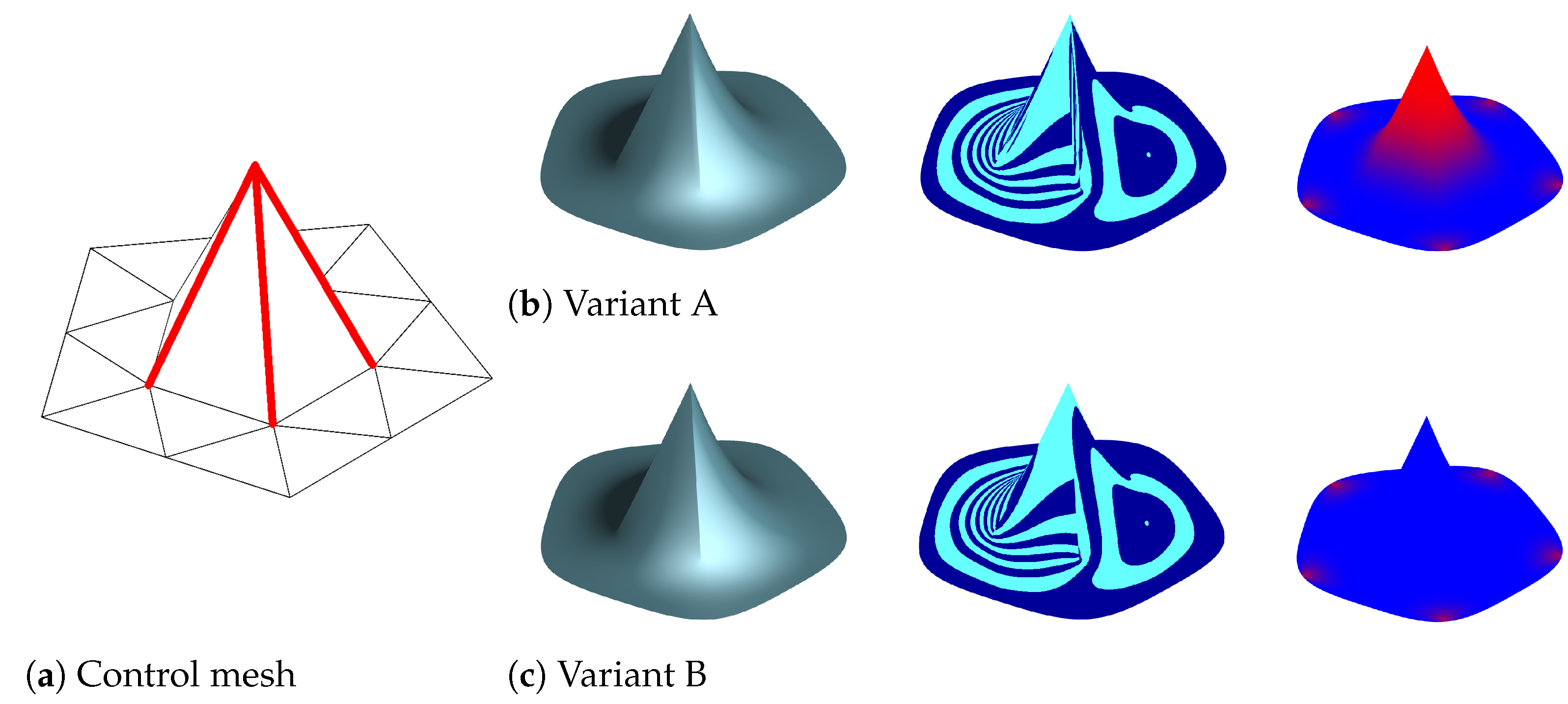
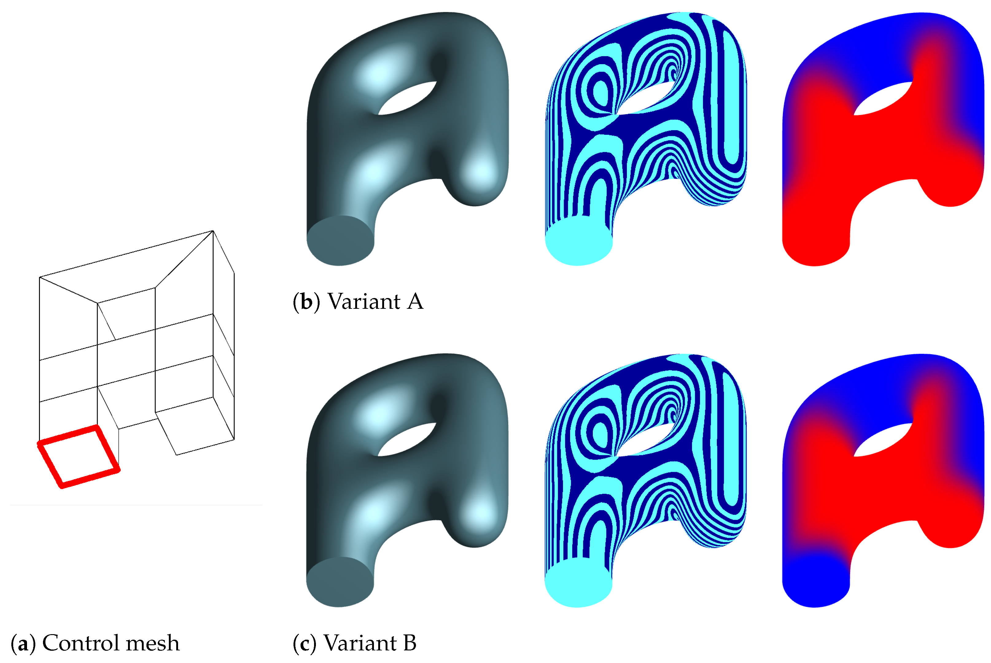
3.1. Blending at Sharp Vertices

The normal field blending method (Section 2.3) does not directly support (semi-)sharp edges. It thus needs to be extended to be able to correctly handle meshes with some of its edges labelled as (semi-)sharp, i.e., to models with (semi-)sharp creases. This means that the blending function definition (see Section 2.3) needs to be extended to account for sharp vertices, i.e., vertices incident with at least two sharp edges.

We emphasise that the ideas and both variants are shared between the Catmull-Clark and Loop subdivision schemes. We investigate two variants for this extension, as follows:

• Variant A: We treat sharp vertices as standard (smooth) vertices. In other words, initialising extraordinary sharp vertices (and possibly their one ring neighborhood) with control blending weights that will lead to the value of 1 in the limit (see Section 2.3), and initialising regular sharp vertices with 0.
• Variant B: We initialise the control blending weights of sharp vertices to 0, no matter whether they are regular vertices or EVs. The idea behind this is that sharp vertices are not meant to look smooth, and thus are not expected to benefit from subdivided normals.

Figure 3 shows the two variants with blend weights visualised using a colour map.

Figure 3. Top row: A tetrahedron model with three sharp edges (red) with sharpness value 4, shown after 4 subdivision steps. Bottom row: A cube model with seven sharp edges (red) with sharpness value 4. From left to right: (a) The control mesh with sharp edges highlighted. (b) The control mesh after 4 subdivision steps. (c) Blend weights using Variant A. (d) Blend weights using Variant B. Blue corresponds to the value of 0 and red to 1 of the limit blending function b. Both models start blending weights at subdivision level 2.

3.2. Blending at Semi-Sharp Vertices

We also need to be able to handle semi-sharp edges and vertices. For an edge with its sharpness value of s, after s steps of subdivision of a model all sharp vertices become smooth vertices. Thus the geometry, normals, and blending weights are all subdivided using the smooth rule in this case. Figure 4 shows the difference of blend weights on sharp versus semi-sharp edges. When the edges are sharp, in fewer than s subdivision steps, weights are all 0 on the (subdivided chain of) edges; when the edge(s) become smooth, after at least s subdivision steps, the weights of EVs are 1 on the (chain of subdivided) edges.

Figure 4. Top row: A 3D cross triangle model with four sharp edges (red) with sharpness value 4, shown after 4 and 5 Loop subdivision steps. Bottom row: A 3D cross quad model with four sharp edges (red) with sharpness value 4, shown after 4 and 5 Catmull-Clark subdivision steps. From left to right: (a) The control mesh with sharp edges highlighted. (b) The control mesh after 4 subdivision steps. (c) Blend weights of the models after 4 subdivision steps using Variant B. Note that there is no blending on vertices on sharp edges. (d) The control mesh after 5 subdivision steps. (e) Blend weights of the models after 5 subdivision steps using Variant B. Now, the normals at EVs on originally semi-sharp edges are blended. For both models, blending of weights starts at subdivision level 2.

After performing s steps of subdivision, the sharp vertices are meant to become smooth, which means that they are expected to benefit from subdivided normals. So we treat them exactly as smooth vertices, and EVs on semi-sharp edges can be shaded smoothly by applying fake normals.

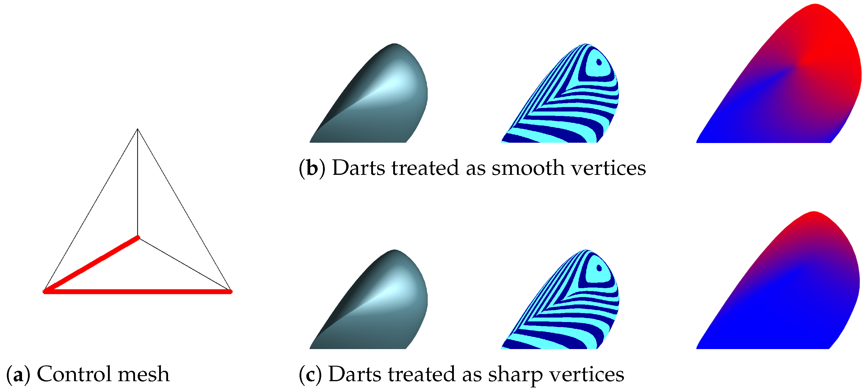
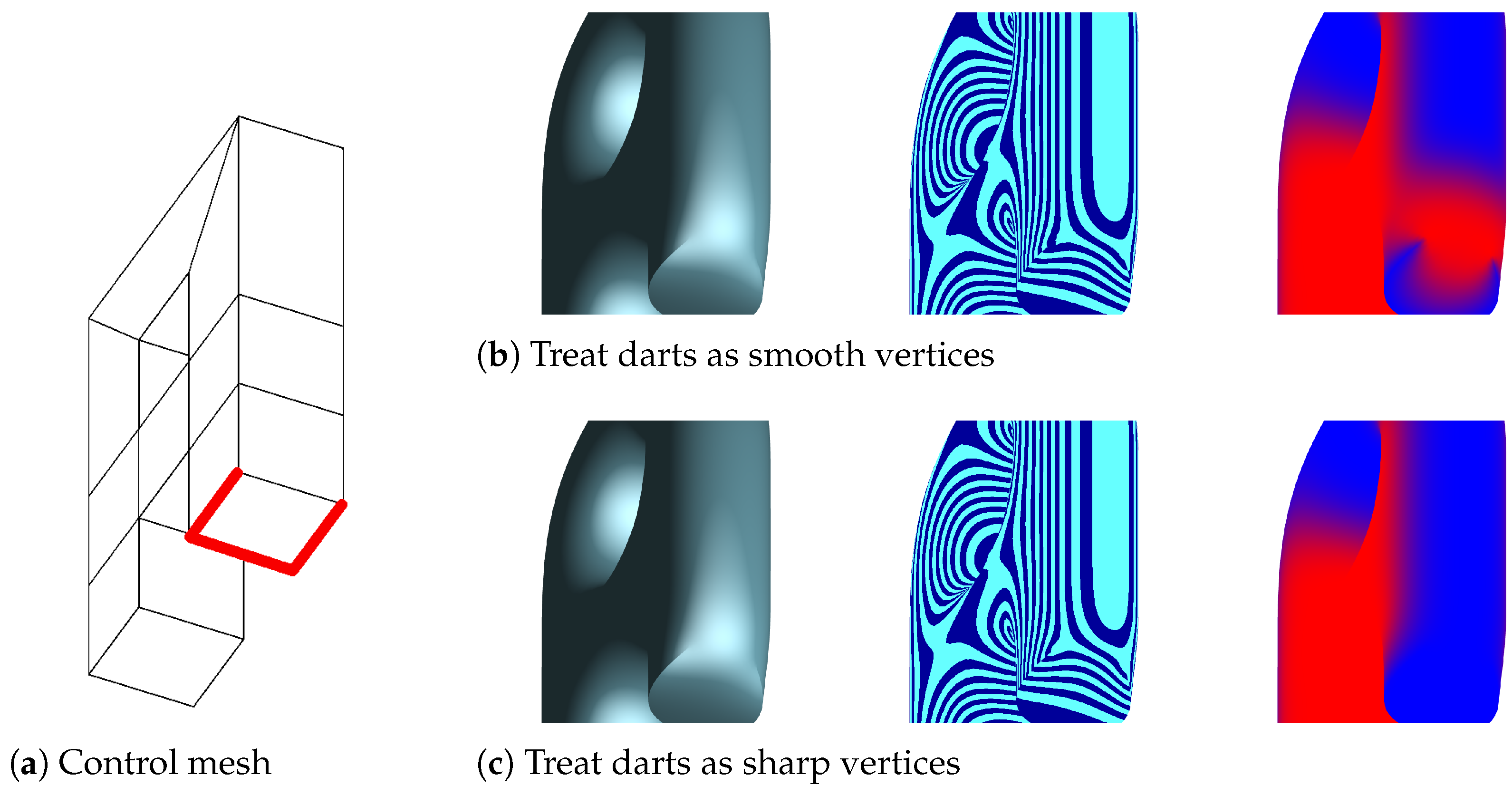
3.3. Blending at Dart Vertices

We now focus on dart vertices, i.e., vertices incident with just one sharp edge. When subdividing the geometry of the mesh, dart vertices are considered smooth. Nevertheless, this does not mean that one should treat normals similarly. We explore two ways: we either consider dart vertices as sharp vertices, or we consider them as smooth vertices.

The above-proposed options cover all sensible variants for treating semi-sharpness or infinite sharpness in combination with subdivision shading. See Figure 5 for a comparison of the two options.

Figure 5. Top row: A tetrahedron model with two sharp edges (red) with sharpness value 4. Bottom row: A cube model with three sharp edges (red) with sharpness value 4. From left to right: (a) The control mesh with sharp edges highlighted. (b) The control mesh after 4 subdivision steps. (c) The blending weights when darts are treated as smooth vertices. (d) The blending weights when darts are treated as sharp vertices.

3.4. Normals at Sharp Vertices

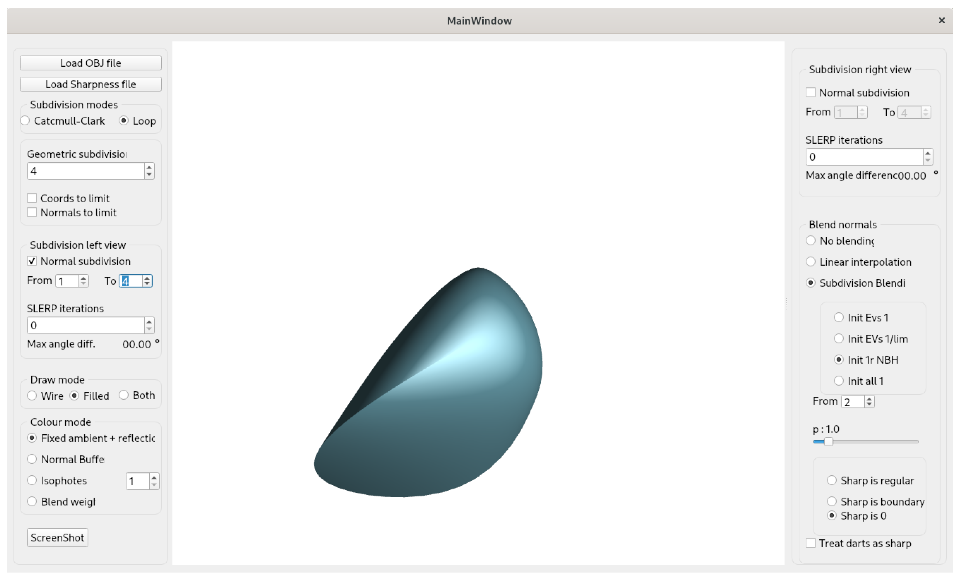
A typical Catmull-Clark or Loop subdivision implementation supports only one normal at each vertex. In contrast, every vertex can have up to n distinct normals in our method, where n specifies the number of sharp edges ending at that vertex; see Figure 6a. This is the case since the normals on both sides of a crease typically disagree, and this should stay the case throughout the subdivision process and also when the limit surface is shaded.

Figure 6. (a) Multiple normals associated with sharp vertices. (b) Regions (in different colours) separated by sharp edges (black solid lines) and non-sharp edges (black dashed lines).

To facilitate this, in the control mesh we assign each sharp vertex (incident with at least two sharp edges) a set of regions. Each region consists of all incident faces that are not separated from each other by a sharp edge (black solid line), as illustrated in Figure 6b. If not specified by the user, the vertex is given a normal for each region; we use the average of the face normals in that region. Subdividing the normals then proceeds as follows. If a subdivision stencil includes a sharp vertex, the regular vertex normal of that vertex is not used. Instead, we use the sharp normal that is in the same region as the (subdivided) normal that is being determined. In our experimental implementation, users have the possibility to set sharpness values directly in the tool’s user interface, or through a modified OBJ file, as described next.

3.5. Implementation

Our implementation is based on that of [4] and our short paper [7]. It uses C++, OpenGL for graphics, and Qt for window and widget design. The program loads models from .OBJ files (with modifications to support (semi-)sharp edges) into the half-edge data structure [13].

Vertex normals are calculated as the average of the surrounding face normals, with the exception of sharp vertices; see Figure 6. It then subdivides the mesh a user-defined number of times using Catmull-Clark or Loop subdivision. The sharpness values of edges, as described in Section 2.1, are defined in .OBJ files (or default to zero), and are stored for later use for geometry and normal vector subdivision. More specifically, for each face in the file, we add a list of sharpness values. Each such line consists of either of the following two options:

• fs x, where x is a sequence of digits specifying the sharpness values of the edges of a face in clockwise order. For example: fs 1 2 3 2 5.
• as y x: x is the same as above and y is a positive integer. This will assign the sharpness values x to the next y faces in the list.

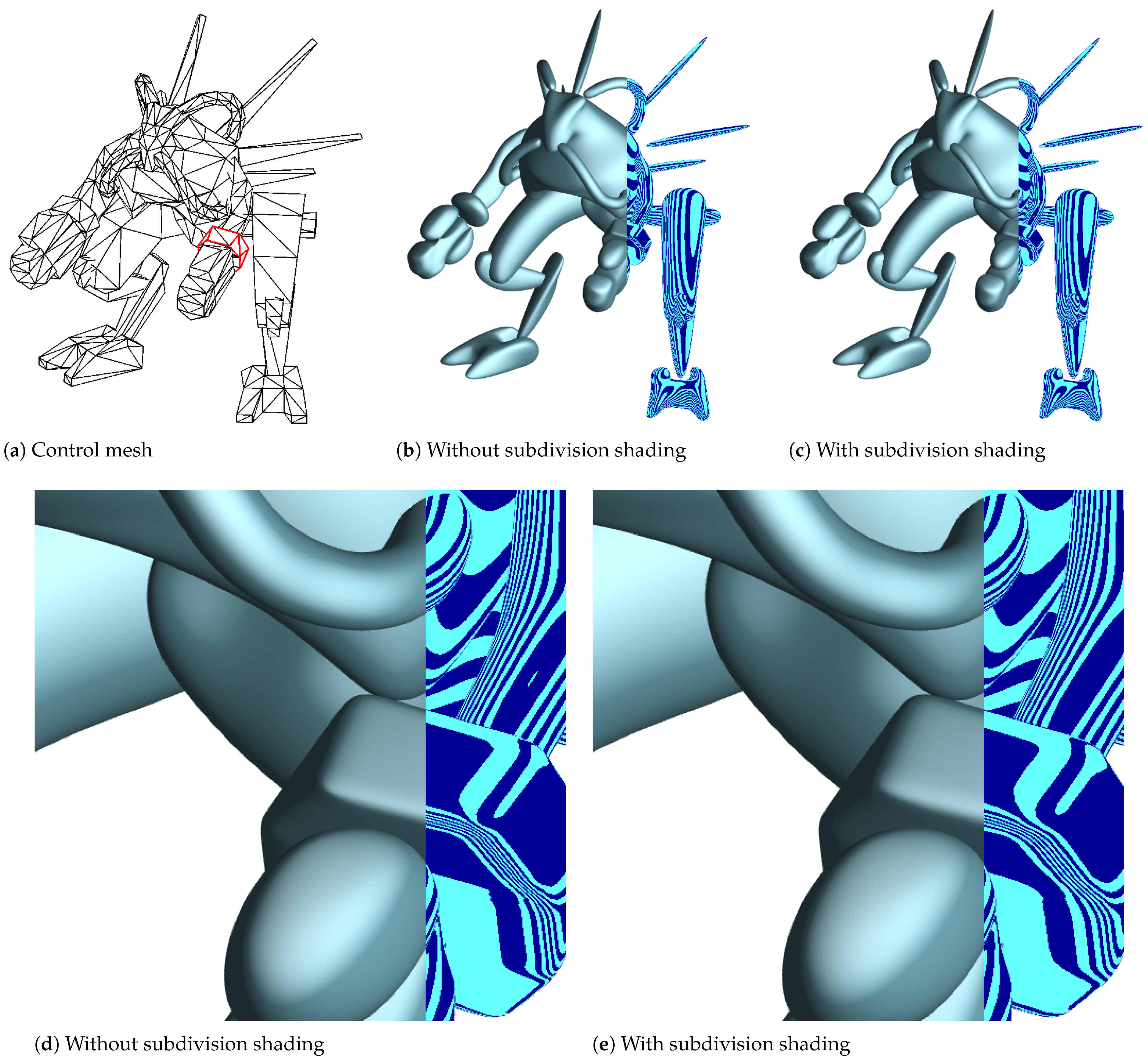
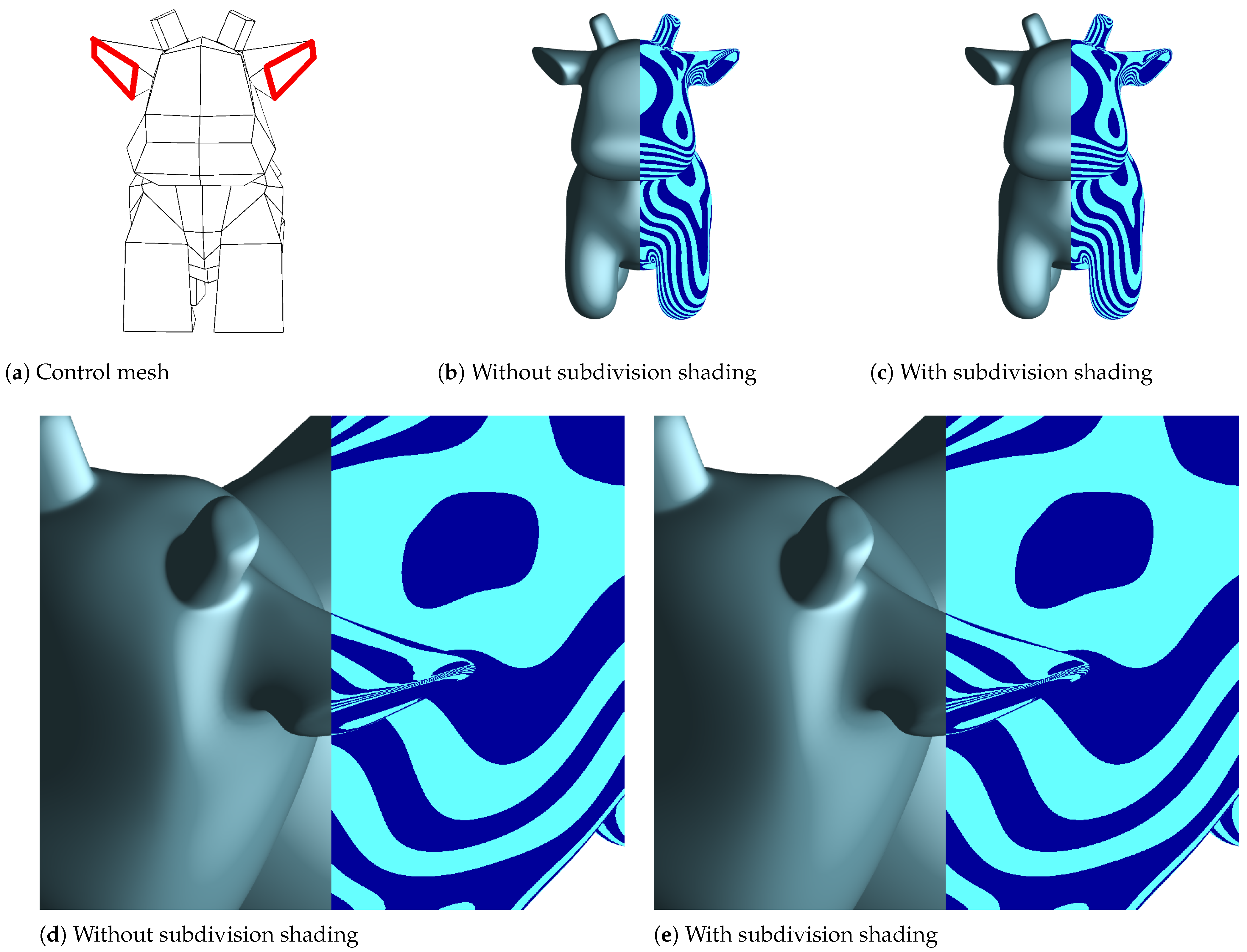
If not all faces are covered by this sharpness specification, the remaining sharpness values in the model will be set to 0. In case two faces specify different values for an edge they share, the highest value will be used. This case cannot occur when using our tool, but it can arise when editing the (modified) .OBJ file directly by hand. An alternative would be to specify sharpness values per edge, but this would require an explicit storing of edges in the files.

The user is provided with a set of UI options to control the settings of the subdivision and blending of the normals based on Equation (1) and the blending methods specified in Section 3.1. The bottom right menu enables users to specify how the blend weights of sharp vertices should be treated, allowing them to choose between either setting those weights to 0 or to treat sharp vertices the same way as regular vertices. Below it, the users can specify whether darts should be treated as sharp vertices or as regular vertices (see Section 3.3). The tool has options also to visualise certain aspects of the mesh, such as the blend weights, the normal buffers, or highlight lines. The user interface of our experimental tool is shown in Figure 7. We used the tool to generate all examples in this paper.

Figure 7. User interface of the experimental tool.

4. Results

We now demonstrate our method on several results and provide comparisons of the proposed subdivision shading variants.

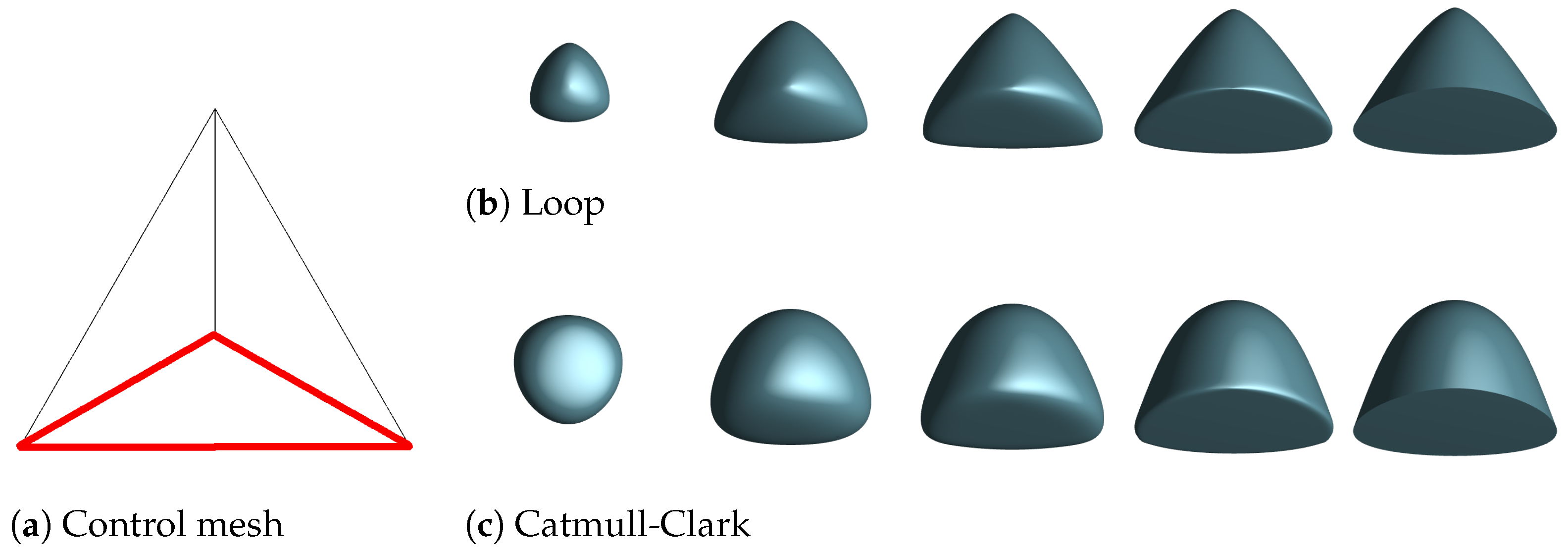
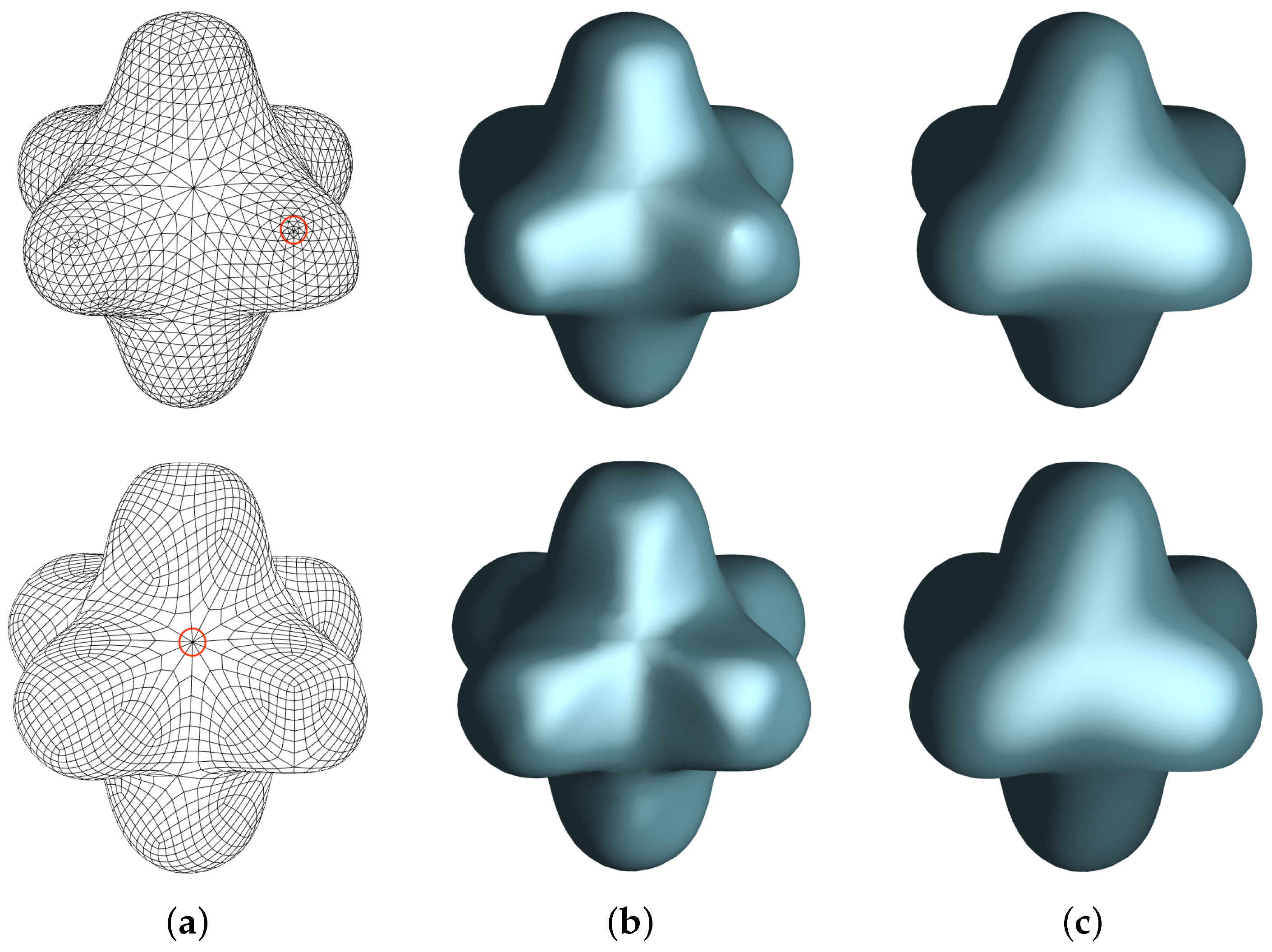
4.1. Catmull-Clark and Loop Subdivision Results

We start with the Robot model in combination with the Loop subdivision scheme in Figure 8, and the Spot model subdivided using the Catmull-Clark scheme in Figure 9. They show the differences between using Loop and Catmull-Clark subdivision combined with semi-sharp creases without and with our method.

Figure 8. Top row: (a) The Robot model with semi-sharp edges of sharpness value of 2 (shown in red in the control mesh) around its left ‘wrist’. The subdivision level is set to 4. (b) The result without subdivision shading and (c) with subdivision shading using Variant B. Bottom row: (d) The result zoomed in without subdivision shading and (e) with subdivision shading using Variant B. In this example, subdivision of blending weights starts from level 1. The result of Variant B appears smoother, as evidenced by the smoother blue-cyan highlight lines.

Figure 9. Top row: (a) The Spot model with semi-sharp edges of sharpness value of 2 (shown in red in the control mesh) around Spot’s ears. The subdivision level is set to 4. (b) The result without subdivision shading and (c) with subdivision shading using Variant B. Bottom row: (d) The result zoomed in without subdivision shading and (e) with subdivision shading using Variant B. In this example, subdivision of blending weights starts from level 1. The result of Variant B appears smoother (as noticeable in the blue-cyan highlight line rendering of Spot’s left ear).

Our results suggest that for both subdivision methods, using subdivision shading with Variant B produces smoother results than the original respective methods without our subdivision shading. This is especially visible in the highlight line visualisations (in our figures using blue and cyan), which clearly show changes in the normal fields of the generated surfaces.

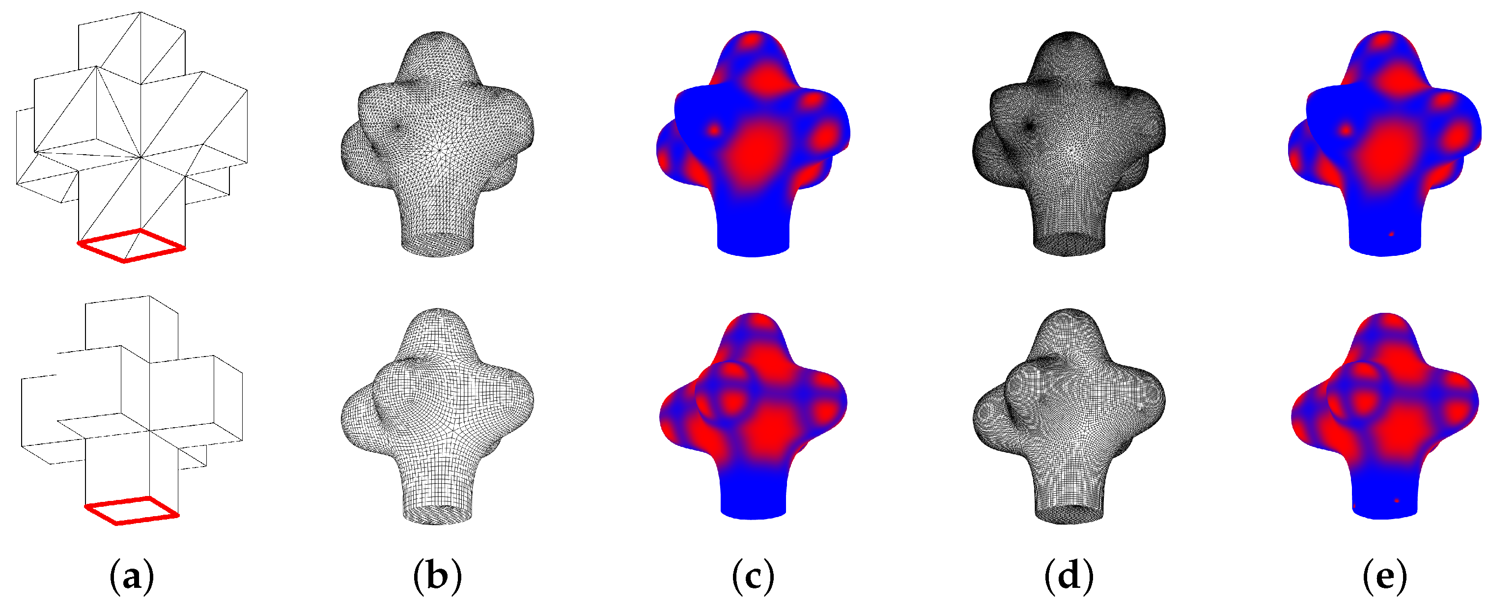
4.2. Blend Weights at Creases with the Two Variants

We tested the two variants on models containing sharp edges. Figure 10 shows a comparison between the two methods on a model with two ‘faces’ composed of sharp edges using Loop subdivision. A clear difference is observable around the sharp faces. When sharp vertices are treated as regular ones (Variant A; top row), the normals misbehave around the sharp edges. This problem does not exist when sharp vertices are initialized with a blend weight of zero (Variant B; bottom row). This is even clearer in the highlight lines plots: in the top image, the lines form wiggles around the sharp edges, while in the bottom image the lines are smoother all the way up to the sharp edges.

Figure 10. Loop subdivision. (a) There are three sharp edges of sharpness value of 4 (shown in red in the control mesh) in the hat model. The subdivision level is set to 4. The results in the top row (b) are the shading, highlight lines, and blend weights using Variant A, and the bottom row (c) using Variant B. In the far right column, blue corresponds to the value of 0 and red to 1 of the limit blending function b; see Equation (1). In this example, subdivision of blending weights starts from level 1.

A similar comparison is made in Figure 11, this time using Catmull-Clark subdivision on a 3D Letter A model. Although the results of the two variants look more similar than in the previous example, Variant B again offers smoother highlight lines, especially leading up to the sharp face. In the case of Variant A, the highlight lines noticeably wiggle when leading up to the sharp face of the model.

Figure 11. Catmull-Clark subdivision. (a) There are four sharp edges of sharpness value of 4 (shown in red in the control mesh) in the Letter A model which make up one planar rounded face. The subdivision level is set to 4. The results in the top row (b) are the shading, highlight lines, and blend weights using Variant A, and the bottom row (c) using Variant B. In the far right column, blue corresponds to the value of 0 and red to 1 of the limit blending function b; see (1). In this example, subdivision of blending weights starts from level 1.

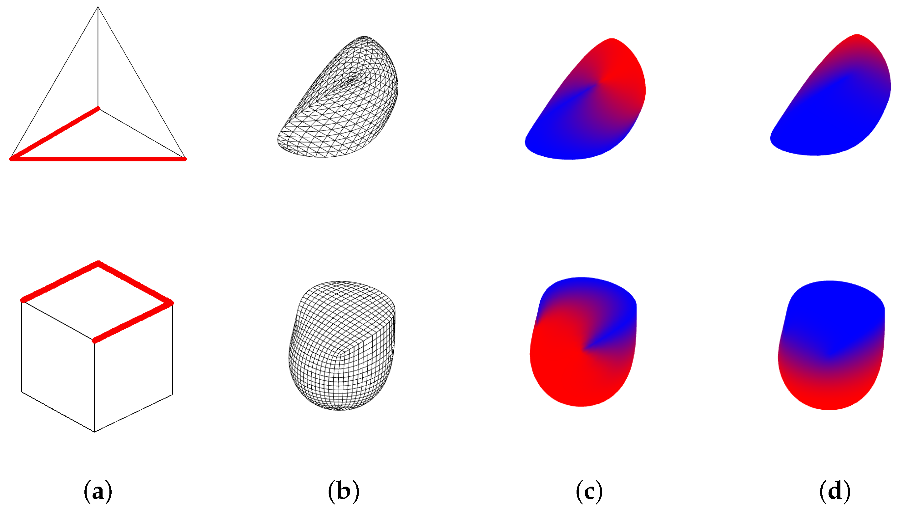
4.3. Blend Weights at Darts

We subdivided models containing darts and compared the results when either treating them as sharp vertices or as non-sharp vertices when initializing the blend weights; see Figure 12 and Figure 13 for examples of Loop and Catmull-Clark subdivision, respectively. Our blending algorithm produces small differences in the resulting shaded meshes around the darts.

Figure 12. (a) The tetrahedron model with two sharp edges. We show the difference between treating darts as smooth vertices (b) or as sharp vertices (c) when setting the blend weights.

Figure 13. (a) The Letter A model with three sharp edges. We show the difference between treating darts as regular vertices (b) or as sharp vertices (c) when setting the blend weights.

When treating the dart as a sharp vertex when subdividing the normals (bottom rows in the figures), the highlight lines clearly show that more sharpness is preserved around the sharp edge. However, this is typically not desirable since the sharp edge ends at the dart vertex and therefore the normal field should transition from being sharp along the creases to smooth towards the dart vertex. Based on this, we argue that it is better to treat darts as smooth vertices (top rows in the figures). However, if a dart vertex is also an EV, we treat it as an EV. This again ensures that the artifacts that normally appear near EVs are mitigated.

5. Discussion

In general, based on our results presented in the previous section, we generally recommend Variant B for use with both Loop and Catmull-Clark subdivision surfaces with (semi-)sharp creases. On top of this, we recommend to treat dart vertices as smooth vertices (unless they are extraordinary vertices) for the purposes of subdivision shading.

When using our blending scheme, the weights away from EVs are all set to 0, which means that, after subdivision, fewer and fewer vertices have a positive blend weight. This, in turn, means that subdivided normals do not need to be calculated at those vertices. In other words, the subdivided normal has to be calculated only in the vicinity of vertices where the blending weight is initialised to 1, as it has no influence on the shading result elsewhere.

For example, if we subdivide the Spot model (see Figure 9) up to level 4, the total number of vertices is 46,850. If we start blending from level 4, taking into account the model’s EVs (of valency 3 and 5) and their neighbourhoods with non-zero blending weights at level 4 when relying on the inverse limit stencil approach [4], we end up with only 832 vertices for which subdivided normals are needed and used. This is less than $1.8\%$ of the total, resulting in big computational savings in the normal subdivision and blending efforts compared to naive implementations. When using the variant of setting all blending weights at EVs and their neighbours to the value of 1 (see Section 2.2), then this count is 2304, giving $5\%$ of the total.

In cases where a model contains no infinitely sharp creases, the efficiency of our method is the same as that of the original subdivision shading relying on linear averaging of normals. However, in the case of models with sharp creases, it can no longer rely on indexed rendering due to the multiple normals being associated with some of the vertices, which is of course the case for all methods dealing with sharp creases, which in turn makes the method marginally slower. Consider the theoretically extreme situation of the Spot model (see Figure 9), assuming all its edges were infinitely sharp and with subdivision up to level 4. The total number of vertices would (still) be 46,850, but we would now have to consider multiple normals for all these vertices. This would naturally be much slower than the original subdivision shading method.

In practice, infinitely sharp creases are rarely used as they lead to (other) issues, such as when using displacement maps. Instead, they are often replaced with semi-sharp creases with a finite sharpness value. However, this does not suggest that rules for sharp vertices/edges are not useful. To the contrary, sharp rules are still needed to be able to handle semi-sharp creases in the subdivision process without using large amounts of extra vertices. As we mentioned in Section 3.2, many production models come with semi-sharp creases, meaning that sharp edges of sharpness value of s are then subdivided using the smooth rule and thus can benefit from subdivision shading if there are EVs on the creases.

Finally, note that while we have presented results based on both the Catmull-Clark and the Loop subdivision schemes, the ideas in our method directly apply to other schemes (such as those of high-degree approximating subdivision schemes [14] or based on hexagonal elements [15]).

6. Conclusions

In this paper, we have proposed extensions to subdivision shading to make it applicable also to models including (semi-)sharp creases. This is a powerful combination of subdivision shading [3,4] and semi-sharp creases [5] in Catmull-Clark, Loop, and potentially other subdivision schemes.

We have investigated two options for setting the control blending weights of sharp vertices. Based on our results, we have observed that in most cases initialising the weights to zero produces better shading in the regions near sharp creases. This agrees with our expectations since the normal blending equation strives to ensure that the limit surface appears $C^1$ smooth globally, while it actually should not be so near sharp edges by definition.

Further to this, according to our experiments, dart vertices should not be treated as sharp vertices when blending the normals. This is consistent with the way darts are treated when subdividing the geometry/vertices of the mesh, and it produces superior results.

As discussed above, an open question remains in whether setting the weights at sharp vertices can be used to increase the method’s efficiency. This, along with implementing the entire subdivision process using subdivision tables [16], is a promising avenue for future research to speed up our method. Another interesting direction is to investigate how to further reduce the appearance of minor but still existing shading artifacts in some situations at EVs in chains of (semi-)sharp edges.

References

1. Catmull, E.; Clark, J. Recursively generated B-spline surfaces on arbitrary topological meshes. Comput.-Aided Des. 1978, 10, 350–355. [Google Scholar] [CrossRef]
2. Loop, C. Smooth Subdivision for Surfaces Based on Triangles. Master’s Thesis, University of Utah, Salt Lake City, UT, USA, 1987. [Google Scholar]
3. Alexa, M.; Boubekeur, T. Subdivision shading. In Proceedings of the ACM Siggraph Asia, Singapore, 10–13 December 2008; pp. 1–4. [Google Scholar]
4. Bakker, J.; Barendrecht, P.; Kosinka, J. Smooth Blended Subdivision Shading. In Proceedings of the Eurographics (Short Papers), Delft, The Netherlands, 16–20 April 2018; pp. 37–40. [Google Scholar]
5. DeRose, T.; Kass, M.; Truong, T. Subdivision surfaces in character animation. In Proceedings of the 25th Annual Conference on Computer Graphics and Interactive Techniques, Orlando, FL, USA, 19–24 July 1998; pp. 85–94. [Google Scholar]
6. Ling, R.; Wang, W.; Yan, D. Fitting Sharp Features with Loop Subdivision Surfaces. Comput. Graph. Forum 2008, 27, 1383–1391. [Google Scholar] [CrossRef]
7. Zhou, J.; Boonstra, J.; Kosinka, J. Semi-Sharp Subdivision Shading; Eurographics Association: Eindhoven, The Netherlands, 2022. [Google Scholar]
8. Kovacs, D.; Mitchell, J.; Drone, S.; Zorin, D. Real-time creased approximate subdivision surfaces. In Proceedings of the 2009 Symposium on Interactive 3D Graphics and Games, New York, NY, USA, 27 February–1 March 2009; pp. 155–160. [Google Scholar]
9. Brainerd, W.; Foley, T.; Kraemer, M.; Moreton, H.; Nießner, M. Efficient GPU rendering of subdivision surfaces using adaptive quadtrees. ACM Trans. Graph. 2016, 35, 1–12. [Google Scholar] [CrossRef]
10. Kosinka, J.; Sabin, M.; Dodgson, N. Subdivision surfaces with creases and truncated multiple knot lines. Comput. Graph. Forum 2014, 33, 118–128. [Google Scholar] [CrossRef]
11. Hoppe, H.; DeRose, T.; Duchamp, T.; Halstead, M.; Jin, H.; McDonald, J.; Schweitzer, J.; Stuetzle, W. Piecewise smooth surface reconstruction. In Proceedings of the Computer Graphics and Interactive Techniques, Orlando, FL, USA, 24–29 July 1994; pp. 295–302. [Google Scholar]
12. Kosinka, J.; Sabin, M.; Dodgson, N. Semi-sharp Creases on Subdivision Curves and Surfaces. Comput. Graph. Forum 2014, 33, 217–226. [Google Scholar] [CrossRef]
13. McGuire, M. The Half-Edge Data Structure. 2000. Available online: https://www.flipcode.com/archives/The_Half-Edge_Data_Structure.shtml (accessed on 20 April 2023).
14. Stam, J. On subdivision schemes generalizing uniform B-spline surfaces of arbitrary degree. Comput. Aided Geom. Des. 2001, 18, 383–396. [Google Scholar] [CrossRef]
15. Barendrecht, P.; Sabin, M.; Kosinka, J. A bivariate C1 subdivision scheme based on cubic half-box splines. Comput. Aided Geom. Des. 2019, 71, 77–89. [Google Scholar] [CrossRef]
16. Dupuy, J.; Vanhoey, K. A Halfedge Refinement Rule for Parallel Catmull-Clark Subdivision. Comput. Graph. Forum 2021, 40, 57–70. [Google Scholar] [CrossRef]
Disclaimer/Publisher’s Note: The statements, opinions and data contained in all publications are solely those of the individual author(s) and contributor(s) and not of MDPI and/or the editor(s). MDPI and/or the editor(s) disclaim responsibility for any injury to people or property resulting from any ideas, methods, instructions or products referred to in the content.
Article Metrics
Citations
Article Access Statistics
Multiple requests from the same IP address are counted as one view.